Computing the Characteristic Polynomial of a Finite Rank Two Drinfeld Module

Abstract.

Motivated by finding analogues of elliptic curve point counting techniques, we introduce one deterministic and two new Monte Carlo randomized algorithms to compute the characteristic polynomial of a finite rank-two Drinfeld module. We compare their asymptotic complexity to that of previous algorithms given by Gekeler, Narayanan and Garai-Papikian and discuss their practical behavior. In particular, we find that all three approaches represent either an improvement in complexity or an expansion of the parameter space over which the algorithm may be applied. Some experimental results are also presented.

1. Introduction

Drinfeld modules were introduced by Drinfeld in (Drinfel’d, 1974) (under the name elliptic modules) to prove certain conjectures pertaining to the Langlands program; they are themselves extensions of a previous construction known as the Carlitz module (Carlitz, 1935).

In this paper, we consider so-called Drinfeld modules of rank two over a finite field $\mathbb{L}$. Precise definitions are given below, but this means that we will study the properties of ring homomorphisms from $\mathbb{F}_{q}[x]$ to the skew polynomial ring $\mathbb{L}\{\tau\}$, where $\tau$ satisfies the commutation relation $\tau u=u^{q}\tau$ for $u$ in $\mathbb{L}$. Here, the rank of such a morphism $\varphi$ is the degree in $\tau$ of $\varphi(x)$.

Rank two Drinfeld modules enjoy remarkable similarities with elliptic curves: analogues exist of good reduction, complex multiplication, etc. Based in part on these similarities, Drinfeld modules have recently started being considered under the algorithmic viewpoint. For instance, they have been proved to be unsuitable for usual forms of public key cryptography (Scanlon, 2001); they have also been used to design several polynomial factorization algorithms (Panchishkin and Potemine, 1989; van der Heiden, 2004; Narayanan, 2018; Doliskani et al., 2017); recent work by Garai and Papikian discusses the computation of their endomorphism rings (Garai and Papikian, 2018). Our goal is to study in detail the complexity of computing the characteristic polynomial of a rank two Drinfeld module over a finite field.

A fundamental object attached to an elliptic curve $E$ defined over a finite field $\mathbb{F}_{q}$ is its Frobenius endomorphism $\pi:(x,y)\mapsto(x^{q},y^{q})$; it is known to satisfy a degree-two relation with integer coefficients called its characteristic polynomial. Much is known about this polynomial: it takes the form $T^{2}-hT+q$, for some integer $h$ called the trace of $\pi$, with $\log_{2}(|h|)\leq\log_{2}(q)/2+1$ (this is known as the Hasse bound). In 1985, Schoof famously designed the first polynomial-time algorithm for finding the characteristic polynomial of such a curve (Schoof, 1985).

Our main objective is to investigate the complexity of a Drinfeld analogue of this question. Given a rank two Drinfeld module over a degree $n$ extension $\mathbb{L}$ of $\mathbb{F}_{q}$, one can define its Frobenius endomorphism, and prove that it satisfies a degree-two relation $T^{2}-AT+B$, where $A$ and $B$ are now in $\mathbb{F}_{q}[x]$. As in the elliptic case, $B$ is rather easy to determine, and of degree $n$. Hence, our main question is the determination of the polynomial $A$, which is known to have degree at most $n/2$ (note the parallel with the elliptic case).

Contrary to the elliptic case, computing the characteristic polynomial of a Drinfeld module is easily seen to be feasible in polynomial time: it boils down to finding the $\Theta(n)$ coefficients of $a$, which are known to satisfy certain linear relations. Gekeler detailed such an algorithm in (Gekeler, 1991); we will briefly revisit it in order to analyse its complexity, which turns out to be cubic in $n$. Our main contributions in this paper are several new algorithms with improved runtimes; we also present experimental results obtained by an implementation based on NTL (Shoup, 2019).

An implementation of Gekeler’s algorithm was described in (Jung, 2000) and used to study the distribution of characteristic polynomials of Drinfeld modules by computing several thousands of them.

2. Preliminaries

In this section, we introduce notation to be used throughout the paper; we recall the basic definition of Drinfeld modules and state precisely our main problem. For a general reference on these questions, see for instance (Goss, 1996).

2.1. The Fields $\mathbb{F}_{q}$, $\mathbb{K}$ and $\mathbb{L}$

In all the paper, $\mathbb{F}_{q}$ is a given finite field, of order a prime power $q$, and $\mathbb{L}\supset\mathbb{F}_{q}$ is another finite field of degree $n$ over $\mathbb{F}_{q}$. Explicitly, we assume that $\mathbb{L}$ is given as $\mathbb{L}=\mathbb{F}_{q}[z]/\mathfrak{f}$, for some monic irreducible $\mathfrak{f}\in\mathbb{F}_{q}[z]$ of degree $n$. When needed, we will denote by $\zeta\in\mathbb{L}$ the class $(z\bmod\mathfrak{f})$.

In addition, we suppose that we are given a ring homomorphism $\gamma:\mathbb{F}_{q}[x]\to\mathbb{L}$. The kernel $\ker(\gamma)$ of the mapping $\gamma:\mathbb{F}_{q}[x]\to\mathbb{L}$ is a prime ideal of $\mathbb{F}_{q}[x]$ generated by a monic irreducible polynomial $\mathfrak{p}$, referred to as the $\mathbb{F}_{q}[x]$-characteristic of $\mathbb{L}$. Then, $\gamma$ induces an embedding $\mathbb{K}:=\mathbb{F}_{q}[x]/\mathfrak{p}\to\mathbb{L}$; we will write $m:=[\mathbb{L}:\mathbb{K}]$, so that $n=md$, with $d=\deg\mathfrak{p}$. When needed, we will denote by $\xi\in\mathbb{K}$ the class $(x\bmod\mathfrak{p})$.

Although it may not seem justified yet, we may draw a parallel with this setting and that of elliptic curves over finite fields. As said before, one should see $\mathbb{F}_{q}[x]$ playing here the role of $\mathbb{Z}$ in the elliptic theory. The irreducible $\mathfrak{p}$ is the analogue of a prime integer $p$, so that the field $\mathbb{K}=\mathbb{F}_{q}[x]/\mathfrak{p}$ is often thought of as the “prime field”, justifying the term “characteristic” for $\mathfrak{p}$. The field extension $\mathbb{L}$ will be the “field of definition” of our Drinfeld modules.

We denote by $\pi:\mathbb{L}\to\mathbb{L}$ the $q$-power Frobenius $u\mapsto u^{q}$; for $i\geq 0$, the $i$th iterate $\pi^{i}:\mathbb{L}\to\mathbb{L}$ is thus $u\mapsto u^{q^{i}}$; for $i\leq 0$, $\pi^{i}$ is the $i$th iterate of $\pi^{-1}$.

2.2. Skew Polynomials

We write $\mathbb{L}\{\tau\}$ for the ring of so-called skew polynomials

(1) $$\mathbb{L}\{\tau\} =\{U=u_{0}+u_{1}\tau+\cdots+u_{s}\tau^{s}\ \mid\ s\in\mathbb{N},u_{0},\dots,u_{s}\in\mathbb{L}\}.$$

This ring is endowed with the multiplication induced by the relation $\tau u=u^{q}\tau$, for all $u$ in $\mathbb{L}$. Elements of $\mathbb{L}\{\tau\}$ are sometimes called linearized polynomials, since there exists an isomorphism mapping $\mathbb{L}\{\tau\}$ to polynomials of the form $u_{0}x+u_{1}x^{q}+\cdots+u_{s}x^{q^{s}}$, which form a ring for the operations of addition and composition.

A non-zero element $U$ of $\mathbb{L}\{\tau\}$ admits a unique representation as in (1) with $u_{s}$ non-zero. Its degree $\deg U$ is the integer $s$ (as usual, we set $\deg 0=-\infty$). The ring $\mathbb{L}\{\tau\}$ admits a right Euclidean division: given $U$ and $V$ in $\mathbb{L}\{\tau\}$, with $V$ non-zero, there exists a unique pair $(Q,R)$ in $\mathbb{L}\{\tau\}^{2}$ such that $U=QV+R$ and $\deg R<\deg V$.

There is a ring homomorphism $\iota:\mathbb{L}\{\tau\}\to{\rm End}_{\mathbb{F}_{q}}[\mathbb{L}]$ given by

$$\iota:u_{0}+u_{1}\tau+\dots+u_{s}\tau^{s}\mapsto u_{0}{\rm Id}+u_{1}\pi+\dots+u_{s}\pi^{s},$$

where $\rm{Id}:\mathbb{L}\to\mathbb{L}$ is the identity operator and $\pi$ and its powers are as defined above. This mapping allows us to interpret elements in $\mathbb{L}\{\tau\}$ as $\mathbb{F}_{q}$-linear operators $\mathbb{L}\to\mathbb{L}$.

2.3. Drinfeld Modules

Drinfeld modules can be defined in a quite general setting, involving projective curves defined over $\mathbb{F}_{q}$; we will be concerned with the following special case (where the projective curve in question is simply $\mathbb{P}^{1}$).

Definition 0.

Let $\mathbb{L}$ and $\gamma$ be as above. A rank $r$ Drinfeld module over $(\mathbb{L},\gamma)$ is a ring homomorphism $\varphi:\mathbb{F}_{q}[x]\to\mathbb{L}\{\tau\}$ such that

$$\varphi(x)=\gamma(x)+u_{1}\tau+\cdots+u_{r}\tau^{r},$$

with $u_{1},\dots,u_{r}$ in $\mathbb{L}$ and $u_{r}$ non-zero.

For $U$ in $\mathbb{F}_{q}[x]$, we will abide by the convention of writing $\varphi_{U}$ in place of $\varphi(U)$. Since $\varphi$ is a ring homomorphism, we have $\varphi_{UV}=\varphi_{U}\varphi_{V}$ and $\varphi_{U+V}=\varphi_{U}+\varphi_{V}$ for all $U,V$ in $\mathbb{F}_{q}[x]$; hence, the Drinfeld module $\varphi$ is determined entirely by $\varphi_{x}$; precisely, for $U$ in $\mathbb{F}_{q}[x]$, we have $\varphi_{U}=U(\varphi_{x})$.

We will restrict our considerations to rank two Drinfeld modules. In particular, we will use the now-standard convention of writing $\varphi_{x}=\gamma(x)+g\tau+\Delta\tau^{2}$. Hence, for a given $(\mathbb{L},\gamma)$, we can represent any rank two Drinfeld module over $(\mathbb{L},\gamma)$ by the pair $(g,\Delta)\in\mathbb{L}^{2}$.

Example 0.

Let $q=5$, $\mathfrak{f}=z^{4}+4z^{2}+4z+2$ and $\mathbb{L}=\mathbb{F}_{5}[z]/\mathfrak{f}=\mathbb{F}_{625}$, so that $n=4$; we let $\zeta$ be the class of $z$ in $\mathbb{L}$. Let $\gamma:\mathbb{F}_{5}[x]\to\mathbb{F}_{625}$ be given by $x\mapsto\zeta$, so that $\mathfrak{p}=\mathfrak{f}$, $\mathbb{K}=\mathbb{L}=\mathbb{F}_{625}$ and $m=1$. We define the Drinfeld module $\varphi:\mathbb{F}_{5}[x]\to\mathbb{F}_{625}\{\tau\}$ by $\varphi_{x}=\zeta+\tau+\tau^{2}$, so that $(g,\Delta)=(1,1)$.

Suppose $\varphi$ is a rank two Drinfeld module over $(\mathbb{L},\gamma)$. A central element in $\mathbb{L}\{\tau\}$ is called an endormorphism of $\varphi$. Since $u^{q^{n}}=u$ for all $u$ in $\mathbb{L}$, $\tau^{n}$ is such an endomorphism. The following key theorem (Gekeler, 1991, Cor. 3.4) defines the main objects we wish to compute.

Theorem 3.

There is a polynomial $T^{2}-AT+B\in\mathbb{F}_{q}[x][T]$ such that $\tau^{n}$ satisfies the equation

(2) $$\tau^{2n}-\varphi_{A}\tau^{n}+\varphi_{B}=0,$$

with $\deg A\leq n/2$ and $\deg B=n$.

The polynomials $A$ and $B$ are respectively referred to as the Frobenius trace and Frobenius norm of $\varphi$. Note in particular the similarity with Hasse’s theorem for elliptic curves over finite fields regarding the respective “sizes” (degree, here) of the Frobenius trace and norm. The main goal of this paper is then to find efficient algorithms to solve the following problem.

Problem 1.

Given a rank two Drinfeld module $\varphi=(g,\Delta)$, compute its Frobenius trace $A$ and Frobenius norm $B$.

Example 0.

In the previous example, we have $A=3x^{2}+x+3$ and $B=x^{4}+4x^{2}+4x+2$.

By composing $\varphi:\mathbb{F}_{q}[x]\to\mathbb{L}\{\tau\}$ and $\iota:\mathbb{L}\{\tau\}\to{\rm End}_{\mathbb{F}_{q}}[\mathbb{L}]$ as defined in the previous subsection, we obtain another ring homomorphism $\Phi:\mathbb{F}_{q}[x]\to{\rm End}_{\mathbb{F}_{q}}[\mathbb{L}]$; we will use the same convention of writing $\Phi_{U}=\Phi(U)$ for $U$ in $\mathbb{F}_{q}[x]$. Thus, we see that a Drinfeld module equips $\mathbb{L}$ with a new structure as an $\mathbb{F}_{q}[x]$-module, induced by the choice of $\Phi_{x}=\gamma(x){\rm Id}+g\pi+\Delta\pi^{2}$, with $\pi:\mathbb{L}\to\mathbb{L}$ the $q$-power Frobenius map

Applying $\iota$ to the equality in Theorem 3, we obtain that $\pi^{2n}+\Phi_{A}\pi^{n}+\Phi_{B}$ is the zero linear mapping $\mathbb{L}\to\mathbb{L}$. Since $\pi^{n}$ is the identity map, and since we have $\Phi_{A}=A(\Phi_{x})$, $\Phi_{B}=B(\Phi_{x})$, this implies that the polynomial $1-A+B\in\mathbb{F}_{q}[x]$ cancels the $\mathbb{F}_{q}$-endormorphism $\Phi_{x}$. Actually, more is true: $1-A+B$ is the characteristic polynomial of this endomorphism (Gekeler, 1991, Th. 5.1). As it turns out, finding the Frobenius norm $B$ is a rather easy task (see Section 4); as a result, Problem 1 can be reduced to computing the characteristic polynomial of $\Phi_{x}$.

This shows in particular that finding $A$ and $B$ can be done in $(n\log q)^{O(1)}$ bit operations (in all the paper, we will use a boolean complexity model, which counts the bit complexity of all operations on a standard RAM). The questions that interest us are to make this cost estimate more precise, and to demonstrate algorithmic improvements in practice, whenever possible. Our main results are as follows.

Theorem 5.

One can solve Problem 1

• in Monte Carlo time $(n^{1.885}\log q+n\log^{2}q)^{1+o(1)}$, if the minimal polynomial of $\Phi_{x}$ has degree $n$ (Section 5);

• in time $(n^{2+\varepsilon}\log q+n\log^{2}q)^{1+o(1)}$, for any $\varepsilon>0$ (Section 6);

• in Monte Carlo time $(n^{2}\log^{2}q)^{1+o(1)}$ (Section 7).

Section 4 reviews previous work; it shows that our results are the best to date, except when $\mathbb{K}=\mathbb{L}$ (the “prime field case”), where a runtime $(n^{1.5+\varepsilon}\log q+n^{1+\epsilon}\log^{2}q)^{1+o(1)}$ is possible for any $\varepsilon>0$ (Doliskani et al., 2017). Section 8 discusses the practical behavior of these algorithms; in particular, it highlights that among all of them, the Monte Carlo algorithm of Section 7 features the best runtimes, except when $\mathbb{K}=\mathbb{L}$, where the above-mentioned result of (Doliskani et al., 2017) is superior.

Input and output sizes are $\Theta(n\log q)$ bits, so the best we could hope for is a runtime quasi-linear in $n\log q$; as the theorem shows, we are rather far from this, since the best unconditional results are quadratic in $n$. On the other hand, Problem 1 is very similar to questions encountered when factoring polynomials over finite fields, and it was not until the work of Kaltofen and Shoup (Kaltofen and Shoup, 1998) that subquadratic factorization algorithms were discovered. We believe that finding an algorithm of unconditional subquadratic time in $n$ for Problem 1 is an interesting and challenging question.

The algorithm of Section 6 was directly inspired by Schoof’s algorithm for elliptic curves. We believe this interaction has the potential to yield further algorithms of interest, perhaps using other “elliptic” techniques, such as $p$-adic approaches (Satoh, 2000) or Harvey’s amortization techniques (Harvey, 2014).

3. Algorithmic Background

We now discuss the cost of operations in $\mathbb{L}$ and $\mathbb{L}\{\tau\}$ with runtimes given in bit operations. Notation ($\mathbb{F}_{q},\mathbb{L},\dots$) is as in 2.1. To simplify cost analyses, we assume that $x^{q}\bmod\mathfrak{p}$ is known; we will see below the cost of computing it once and for all, at the beginning of our algorithms.

3.1. Polynomial and matrix arithmetic

3.1.1. Elements of $\mathbb{L}$ are written on the power basis $1,\zeta,\dots,\zeta^{n-1}$. On occasion, we use $\mathbb{F}_{q}$-linear forms $\mathbb{L}\to\mathbb{F}_{q}$; they are given on the dual basis, that is, by their values at $1,\zeta,\dots,\zeta^{n-1}$.

Using FFT-based multiplication, polynomial multiplication, division and extended GCD in degree $n$, and thus addition, multiplication and inversion in $\mathbb{L}$, can be done in $(n\log q)^{1+o(1)}$ bit operations (Gathen and Gerhard, 2013). In particular, computing $x^{q}\bmod\mathfrak{p}$ by means of repeated squaring takes $(n\log^{2}q)^{1+o(1)}$ bit operations.

3.1.2. We let $\omega$ be such that over any ring, square matrix multiplication in size $s$ can be done in $O(s^{\omega})$ ring operations; the best known value to date is $\omega\leq 2.373$ (Coppersmith and Winograd, 1990; Le Gall, 2014). Using block techniques, multiplication in sizes $(s,t)\times(t,u)$ takes $O(stu\min(s,t,u)^{\omega-3})$ ring operations. For matrices over $\mathbb{F}_{q}$, this is $(stu\min(s,t,u)^{\omega-3}\log q)^{1+o(1)}$ bit operations; over $\mathbb{L}$, it becomes $(stu\min(s,t,u)^{\omega-3}n\log q)^{1+o(1)}$.

We could sharpen our results using the so-called exponent $\omega_{2}$ of rectangular matrix multiplication in size $(s,s)\times(s,s^{2})$. We can of course take $\omega_{2}\leq\omega+1\leq 3.373$, but the better result $\omega_{2}\leq 3.252$ is known (Le Gall and Urrutia, 2018). We will not use these refinments in this paper.

3.1.3. Of particular interest is an operation called modular composition, which maps $(F,G,H)\in\mathbb{F}_{q}[x]^{3}$ to $F(G)\bmod H$, with $\deg H=n$ and $\deg F,\deg G<n$. Let $\theta\in[1,2]$ be such that this can be done in $(n^{\theta}\log q)^{1+o(1)}$ bit operations for inputs of degree $O(n)$.

Modular composition is linear in $F$; we also require that its transpose map can be computed in the same runtime $(n^{\theta}\log q)^{1+o(1)}$. In an algebraic model, counting $\mathbb{F}_{q}$-operations at unit cost, the transposition principle (Kaminski et al., 1988) guarantees this, but this is not necessarily the case in our bit model, hence our extra requirement.

For long, the best known value for $\theta$ was Brent and Kung’s $\theta=(\omega+1)/2$ (Brent and Kung, 1978). A major result by Kedlaya and Umans proves that we can actually take $\theta=1+\varepsilon$, for any $\varepsilon>0$ (Kedlaya and Umans, 2011). In practical terms, we are not aware of an implementation of Kedlaya and Umans’ algorithm that would be competitive: for practical purposes, $\theta$ is either $(\omega+1)/2$ (for deterministic approaches) or $(\omega+2)/3$, and $\omega$ itself is either 3 or Strassen’s $\log_{2}7\simeq 2.81$.

3.1.4. A useful application of modular composition is the application of any power of the Frobenius map $\pi$: given $x^{q}\bmod\mathfrak{p}$, for any $\alpha$ in $\mathbb{L}$ and $i\in\{-(n-1),\dots,n-1\}$, we can compute $\pi^{i}(\alpha)$ for $O(\log n)$ modular compositions, that is, in $(n^{\theta}\log q)^{1+o(1)}$ bit operations. See for instance (Gathen and Shoup, 1992, Algorithm 5.2) or Section 2.2 in (Doliskani et al., 2017).

For small values of $i$, say $i=O(1)$, the computation of $\pi^{i}(\alpha)$ can also be done by repeated squaring, in $(n\log^{2}q)^{1+o(1)}$ bit operations. Since for all implementations we are aware of, $\theta=(\omega+1)/2$, this approach may be preferred for moderate values of $\log q$ (this also applies to the operation in the next paragraph).

3.1.5. The previous item implies that if $\varphi=(g,\Delta)$ is a rank two Drinfeld module over $(\mathbb{L},\gamma)$, given $\alpha$ in $\mathbb{L}$, we can compute $\Phi_{x}(\alpha)=\gamma(x)\alpha+g\pi(\alpha)+\Delta\pi^{2}(\alpha)$ in time $(n^{\theta}\log q)^{1+o(1)}$. Because of our requirements on $\theta$, the same holds for the transpose of $\Phi_{x}$: given an $\mathbb{F}_{q}$-linear form $\ell:\mathbb{L}\to\mathbb{F}_{q}$, with the convention of 3.1.1, we can compute the linear form $\Phi_{x}^{\perp}(\ell):\alpha\mapsto\ell(\Phi_{x}(\alpha))$ for the same cost.

3.2. Skew Polynomial Arithmetic

3.2.1. We continue with skew polynomial multiplication. This is an intricate question, with several algorithms co-existing; which one is the most efficient depends on the input degree. We will be concerned with multiplication in degree $k$, for some $k\ll n$; in this case, the best algorithm to date is from (Puchinger and Wachter-Zeh, 2017, Th. 7). For any $k$, that algorithm uses $O(k^{(\omega+1)/2})$ operations $+,\times$ in $\mathbb{L}$, together with $O(k^{3/2})$ applications of powers of the Frobenius, for a total of $(k^{(\omega+1)/2}n^{\theta}\log q)^{1+o(1)}$ bit operations. For higher degrees $k$, the algorithms in (Caruso and Borgne, 2017) have a better runtime.

3.2.2. Our next question is to compute $\varphi_{x^{k}}$, for some $k\geq 0$; this polynomial has $\Theta(k)$ coefficients in $\mathbb{L}$, so it uses $\Theta(kn\log q)$ bits. Since $\varphi_{x^{2k}}=\varphi_{x^{k}}\varphi_{x^{k}}$ and $\varphi_{x^{2k+1}}=\varphi_{x}\varphi_{x^{2k}}$, we can obtain $\varphi_{x^{k}}$ from $\varphi_{x^{\left\lfloor k/2\right\rfloor}}$ using $(k^{(\omega+1)/2}n^{\theta}\log q)^{1+o(1)}$ bit operations. The cumulated time to obtain $\varphi_{x^{k}}$ from $\varphi_{x}$ admits the same upper bound.

3.2.3. We consider now the cost of computing $\varphi_{C}$, for some $C$ in $\mathbb{F}_{q}[x]$. To this end, we adapt the divide-and-conquer algorithm of (Gathen and Gerhard, 2013, Ch. 9), which applies to commutative polynomials.

1. First, choose a power of two $k$ such that $k/2\leq\deg C<k$. We compute $\varphi_{x^{i}}$, for all $i$ powers of two up to $k/2$; using 3.2.2, the cost is $(k^{(\omega+1)/2}n^{\theta}\log q)^{1+o(1)}$.

2. Write $C=C_{0}+x^{k/2}C_{1}$, with $\deg C_{0},\deg C_{1}<k/2$. Compute recursively $\varphi_{C_{0}}$ and $\varphi_{C_{1}}$, and return $\varphi_{C}=\varphi_{C_{0}}+\varphi_{x^{k/2}}\varphi_{C_{1}}$.

The cumulated cost of all recursive calls is $(k^{(\omega+1)/2}n^{\theta}\log q)^{1+o(1)}$, which is $(\deg(C)^{(\omega+1)/2}n^{\theta}\log q)^{1+o(1)}$.

3.2.4. Next, we analyze the cost of computing $\varphi_{1},\varphi_{x},\dots,\varphi_{x^{k}}$, for some $k\geq 0$. In this, we essentially follow a procedure used by Gekeler (Gekeler, 2008, Sec. 3), although the cost analysis is not done in that reference. These polynomials satisfy the following recurrence:

$$\varphi_{x^{i+1}}=\varphi_{x}\varphi_{x^{i}} =(\gamma(x)+g\tau+\Delta\tau^{2})\varphi_{x^{i}}.$$

For $i\geq 0$, write

$$\varphi_{x^{i}}=\sum_{0\leq j\leq 2i}f_{i,j}\tau^{j},$$

for some coefficients $f_{i,j}\in\mathbb{L}$ to be determined. We obtain

$$\sum_{0\leq j\leq 2i}f_{i,j}\tau^{j}=\sum_{0\leq j\leq 2i}\gamma(x)f_{i,j}\tau^{j}+\sum_{j\leq 2i}gf_{i,j}^{q}\tau^{j+1}+\sum_{j\leq 2i}\Delta f_{i,j}^{q^{2}}\tau^{j+2},$$

so the $f_{i,j}$ satisfy the recurrence

$$f_{i+1,j}=\gamma(x)f_{i,j}+gf_{i,j-1}^{q}+\Delta f_{i,j-2}^{q^{2}}$$

with known initial conditions $f_{0,0}=1$, $f_{1,0}=\gamma(x)$, $f_{1,1}=g$, and $f_{1,2}=\Delta$. Evaluating one instance of the recurrence involves $O(1)$ multiplications / additions in $\mathbb{L}$ and applications of the Frobenius map $\pi$, for $(n^{\theta}\log q)^{1+o(1)}$ bit operations. Given $\varphi_{x^{i}}$, there are $\Theta(i)$ choices of $j$, so the overall cost to obtain $\varphi_{1},\varphi_{x},\dots,\varphi_{x^{k}}$ is $(k^{2}n^{\theta}\log q)^{1+o(1)}$ bit operations. In particular, taking $\theta=1+\varepsilon$, we see that the runtime here is essentially linear in the output size, which is $\Theta(k^{2}n\log q)$ bits; this was not the case for the algorithms in 3.2.1 - 3.2.2 - 3.2.3.

However, in 3.1.3, we pointed out that in practice, Brent and Kung’s modular composition algorithm is widely used, with $\theta=(\omega+1)/2$. In this case, for moderate values of $\log q$, one may use the straightforward repeated squaring method to apply the Frobenius map; this leads to a runtime of $(k^{2}n\log^{2}q)^{1+o(1)}$ bit operations, which may be acceptable in practice. This also applies to Proposition 2 below, and underlies the design of the algorithm in Section 7.

3.2.5. We deduce from this an algorithm for inverting $\varphi$. Given $\varphi_{C}=\sum_{0\leq i\leq 2k}\alpha_{i}\tau^{i}$, we want to recover $C=\sum_{0\leq i\leq k}c_{i}x^{i}$ in $\mathbb{F}_{q}[x]$. Writing the expansion

$$\varphi_{C} =\sum_{0\leq i\leq k}c_{i}\sum_{0\leq j\leq 2i}f_{i,j}\tau^{j}=\sum_{0\leq j\leq 2k}\left(\sum_{\lfloor j/2\rfloor\leq i\leq k}c_{i}f_{i,j}\right)\tau^{j}.$$

gives us $2k+1$ equations in $k+1$ unknowns. Keeping only those equations corresponding to even degree coefficients leaves the following upper triangular system of $k+1$ equations over $\mathbb{L}$,

(3) $$\begin{bmatrix}f_{0,0}&f_{1,0}&\ldots&f_{k,0}\\ 0&f_{1,2}&\ldots&f_{k,2}\\ \vdots&\vdots&\ddots&\vdots\\ 0&0&\ldots&f_{k,2k}\end{bmatrix}\begin{bmatrix}c_{0}\\ c_{1}\\ \vdots\\ c_{k}\end{bmatrix}=\begin{bmatrix}\alpha_{0}\\ \alpha_{2}\\ \vdots\\ \alpha_{2k}\end{bmatrix}.$$

Its diagonal entries are of the form $f_{i,2i}$; these are the coefficients of the leading terms of $\varphi_{x^{i}}$, so that for all $i$, $f_{i,2i}=\Delta^{e_{i}}$ for some exponent $e_{i}$. In particular, since $\Delta\neq 0$, the diagonal terms are non-zero, which allows us to find $c_{0},\dots,c_{k}$. Once we know all $f_{i,j}$’s, the cost for solving the system is $O(k^{2})$ operations in $\mathbb{L}$, so the total is $(k^{2}n^{\theta}\log q)^{1+o(1)}$ bit operations.

3.2.6. Finally, we give an algorithm to evaluate a degree $k$ skew polynomial $U$ at $\mu$ elements $\alpha_{1},\dots,\alpha_{\mu}$ in $\mathbb{L}$. This algorithm will be used only in Section 5, so it can be skipped on first reading.

In the case of commutative polynomials, one can compute all $U(\alpha_{i})$ faster than by successive evaluation of $U$ at $\alpha_{1}$, $\alpha_{2}$, …; see (Gathen and Gerhard, 2013, Ch. 10). The same holds for skew polynomial evaluation: in (Puchinger and Wachter-Zeh, 2017, Th. 15), Puchinger and Wachter-Zeh gave an algorithm that uses $O(k^{\max(\log_{2}3,\omega_{2}/2)}\log k)$ operations in $\mathbb{L}$ (including Frobenius-powers applications) in the case $\mu=k$, where $\omega_{2}\leq\omega+1$ as in 3.2.1.

We propose a baby-step / giant-step procedure that applies to any $\mu$ and $k$ (but the cost analysis depends on whether $\mu\leq\sqrt{k}$ or not). Suppose without loss of generality that our input polynomial $U=u_{0}+\cdots+u_{k-1}\tau^{k-1}$ has degree less than $k$, for some perfect square $k$, and let $s=\sqrt{k}$.

1. Commute powers of $\tau$ with the coefficients of $U$ to rewrite it as $U=U^{*}_{0}+\tau^{s}U^{*}_{1}+\cdots+\tau^{s(s-1)}U^{*}_{s-1}$. with all $U^{*}_{i}$ in $\mathbb{L}\{\tau\}$ of degree less than $s$. This is $O(k)$ applications of Frobenius powers in $\mathbb{L}$.

2. Compute $\alpha_{i,j}:=\pi^{i}(\alpha_{j})$, for $i=0,\dots,s-1$ and $j=1,\dots,\mu$; this is $O(s\mu)$ applications of Frobenius powers.

3. For $i<s$, let $u^{*}_{i,0},\dots,u^{*}_{i,s-1}$ be the coefficients of $U^{*}_{i}$. Compute the matrix $(s,s)\times(s,\mu)$ product

   $$\left[\begin{matrix}u^{*}_{0,0}&\cdots&u^{*}_{0,s-1}\\ \vdots&&\vdots\\ u^{*}_{s-1,0}&\cdots&u^{*}_{s-1,s-1}\end{matrix}\right]\left[\begin{matrix}\alpha_{0,1}&\cdots&\alpha_{0,\mu}\\ \vdots&&\vdots\\ \alpha_{s-1,1}&\cdots&\alpha_{s-1,\mu}\end{matrix}\right],$$

   whose entries are the values $\beta_{i,j}:=U^{*}_{i}(\alpha_{j})$. When we apply this result, we will have $\mu\leq s=\sqrt{k}$, so the cost is $O(k\mu^{\omega-2})$ operations in $\mathbb{L}$, by 3.1.2. For completeness, we mention that if $\mu\geq\sqrt{k}$, the cost is $O(k^{(\omega-1)/2}\mu)$ operations in $\mathbb{L}$.

4. Using Horner’s scheme, for $j=1,\dots,\mu$, recover $U(\alpha_{j})$ using $U(\alpha_{j})=\beta_{0,j}+\tau^{s}(\beta_{1,j}+\tau^{s}(\beta_{2,j}+\cdots))$. The total is another $O(s\mu)$ operations in $\mathbb{L}$, including Frobenius powers.

When $\mu\leq\sqrt{k}$, the cost is $(k\mu^{\omega-2}n^{\theta}\log q)^{1+o(1)}$ bit operations. If we take $\mu\geq\sqrt{k}$, the cost becomes $(k^{(\omega-1)/2}\mu n^{\theta}\log q)^{1+o(1)}$.

4. Previous Work on Problem 1

Next, we briefly review existing algorithms for solving Problem 1, and comment on their runtime. Notation are still from Section 2.1.

4.1. Gekeler’s Algorithm

As with elliptic curves, determining the Frobenius norm $B$ of Theorem 3 is simply done using the following result from (Gekeler, 2008, Th. 2.11).

Proposition 1.

Let $N_{\mathbb{L}/\mathbb{F}_{q}}$ be the norm $\mathbb{L}\to\mathbb{F}_{q}$. The Frobenius norm $B$ of a rank two Drinfeld module $\varphi=(g,\Delta)$ over $(\mathbb{L},\gamma)$ is

$$B=(-1)^{n}N_{\mathbb{L}/\mathbb{F}_{q}}(\Delta)^{-1}\mathfrak{p}^{m}.$$

In particular, $B$ can be computed in $(n\log q)^{1+o(1)}$ bit operations. Indeed, $\mathfrak{p}^{m}$ is a degree $n$ polynomial, and we can compute it in the prescribed time by repeated squaring. Moreover $N_{\mathbb{L}/\mathbb{F}_{q}}(\Delta)=\textnormal{resultant}(\mathfrak{f},\Delta)$ (Pohst and Zassenhaus, 1989), so we can compute it in the same time (Gathen and Gerhard, 2013).

Gekeler also gave in (Gekeler, 2008, Sec. 3) an algorithm that determines the Frobenius trace $A$ by solving a linear system for the coefficients of $A$. The key subroutines used in this algorithm were described in the previous section, and imply the following result (the cost analysis is not provided in the original paper).

Proposition 2.

One can solve Problem 1 using $(n^{\theta+2}\log q+n\log^{2}q)^{1+o(1)}$ bit operations.

Proof.

The algorithm is as follows.

1. We compute $x^{q}\bmod\mathfrak{p}$ with $(n\log^{2}q)^{1+o(1)}$ bit operations.

2. Find $\varphi_{1},\dots,\varphi_{x^{n}}$ in $(n^{\theta+2}\log q)^{1+o(1)}$ bit operations (3.2.4).

3. Compute $B$ and deduce $\varphi_{B}$; this takes comparatively negligible time (see above and 3.2.3) and gives us $\varphi_{A}$, since Theorem 3 implies that $\tau^{n}\varphi_{A}=\tau^{2n}+\varphi_{B}.$

4. Recover $A$ in $(n^{\theta+2}\log q)^{1+o(1)}$ bit operations by 3.2.5. ∎

The cost of this procedure is at least cubic in $n$, due to the need to compute the $\Theta(n^{2})$ coefficients $f_{i,j}$ of $\varphi_{1},\dots,\varphi_{x^{n}}$ in $\mathbb{L}$.

4.2. The Case $\mathbb{L}=\mathbb{K}$

The case where $\mathbb{L}=\mathbb{K}$, that is, when $\gamma:\mathbb{F}_{q}[x]\to\mathbb{L}$ is onto, allows for some faster algorithms, based on two observations: we can recover $A$ from its image $\gamma(A)$ in this case (since $\deg A\leq\left\lfloor n/2\right\rfloor$), and $\gamma(A)$ can be easily derived from the Hasse Invariant of $\varphi$, which is the coefficient of $\tau^{n}$ in $\varphi_{\mathfrak{p}}={\mathfrak{p}}(\varphi_{x})$.

From this, Hsia and Yu (Hsia and Yu, 2000) and Garai and Papikian (Garai and Papikian, 2018) sketched algorithms that compute $A$. When $\varphi_{\mathfrak{p}}$ is computed in a direct manner, they take $\Theta(n^{2})$ additions, multiplications and Frobenius applications in $\mathbb{L}$, so $\Omega(n^{3})$ bit operations.

Gekeler (Gekeler, 2008, Prop. 3.7) gave an algorithm inspired by an analogy with the elliptic case, where the Hasse invariant can be computed as a suitable term in a recurrent sequence (with non-constant coefficients). A direct application of this result does not improve on the runtime above. However, using techniques inspired by both the elliptic case (Bostan et al., 2007) and the polynomial factorization algorithm of (Kaltofen and Shoup, 1998), it was shown in (Doliskani et al., 2017) how to reduce the cost to $(n^{\theta+1/2}\log q+n\log^{2}q)^{1+o(1)}$ bit operations, which is subquadratic in $n$.

5. On Narayanan’s Algorithm

In (Narayanan, 2018, Sec. 3.1), Narayanan gives the sketch of a Monte Carlo algorithm to solve Problem 1 for odd $q$, which applies to those Drinfeld modules $(g,\Delta)$ for which the minimal polynomial $\Gamma$ of $\Phi_{x}=\gamma(x){\rm Id}+g\pi+\Delta\pi^{2}$ has degree $n$. In this case, it must coincide with the characteristic polynomial of $\Phi_{x}$, which we saw is equal to $1-A+B$ (this assumption on $\Gamma$ holds for more than half of elements of the parameter domain (Narayanan, 2018, Th. 3.6)). Since $B$ is easy to compute, knowing $1-A+B$ gives us $A$ readily.

Narayanan’s algorithm computes the minimal polynomial $\Gamma_{\ell,\alpha}$ of a sequence of the form $(r_{k})_{k\geq 0}=(\ell(\Phi_{x}^{k}(\alpha))_{k\geq 0}\in{\mathbb{F}_{q}}^{\mathbb{N}}$, for a random $\mathbb{F}_{q}$-linear map $\ell:\mathbb{L}\to\mathbb{F}_{q}$ and a random $\alpha\in\mathbb{L}$. Using Wiedemann’s analysis (Wiedemann, 1986), one can bound below the fraction of $\ell$ and $\alpha$ for which $\Gamma_{\ell,\alpha}=\Gamma$. The bottleneck of this algorithm is the computation of sufficiently many elements of the above sequence: the first $2n$ terms are needed, after which applying Berlekamp-Massey’s algorithm gives us $\Gamma_{\ell,\alpha}$. To compute $(r_{k})_{0\leq k<2n}$, Narayanan states that we can adapt the automorphism projection algorithm of Kaltofen and Shoup (Kaltofen and Shoup, 1998) and enjoy its subquadratic complexity. Indeed, Kaltofen and Shoup’s algorithm computes terms in a similar sequence, namely $\ell(\pi^{k}(\alpha))_{k\geq 0}$, where $\pi$ is the Frobenius map. However, that algorithm actively uses the fact that $\pi$ is a field automorphism, whereas $\Phi_{x}$ is not. Hence, whether a direct adaptation of Kaltofen and Shoup’s algorithm is possible remains unclear to us.

We propose an alternative Monte Carlo algorithm, which establishes the first point in Theorem 5; it is inspired by Coppersmith’s block Wiedemann algorithm (Coppersmith, 1994).

The sequence $(\ell(\Phi_{x}^{k}(\alpha))_{k\geq 0}$ used in Wiedemann’s algorithm is linearly recurrent, so that its generating series is rational, with $\Gamma$ as denominator for generic choices of $\ell$ and $\alpha$. In Coppersmith’s block version, we consider a sequence of $\mu\times\mu$ matrices $({\bm{R}}_{k})_{k\geq 0}$ over $\mathbb{F}_{q}$ instead, for some given parameter $\mu$. These matrices are defined by choosing $\mu$ many $\mathbb{F}_{q}$-linear mappings $\mathbb{L}\to\mathbb{F}_{q}$, say ${\bm{\ell}}=(\ell_{1},\dots,\ell_{\mu})$, and $\mu$ elements ${\bm{\alpha}}=(\alpha_{1},\dots,\alpha_{\mu})$ in $\mathbb{L}$. They define sequences $(r_{i,j,k})_{k\geq 0}:=(\ell_{i}(\Phi_{x}^{k}(\alpha_{j})))_{k\geq 0}$, which form the entries of a sequence of $\mu\times\mu$ matrices $({\bm{R}}_{k})_{k\geq 0}$. The generating series $\sum_{k\geq 0}{\bm{R}}_{k}/z^{k+1}$ can be written as ${\bm{Q}}^{-1}{\bm{N}}$, for some ${\bm{Q}}$ and ${\bm{N}}$ in $\mathbb{F}_{q}[z]^{\mu\times\mu}$. For generic choices of ${\bm{\ell}}$ and ${\bm{\alpha}}$, ${\bm{Q}}$ has degree at most $\lceil n/\mu\rceil$ and can be computed in $(\mu^{\omega-1}n\log q)^{1+o(1)}$ bit operations from $({\bm{R}}_{k})_{k\leq 2n/\mu}$, using the PM basis algorithm of (Giorgi et al., 2003). Finally, we will see that we can deduce the minimal polynomial $\Gamma$ from the determinant of ${\bm{Q}}$.

Thus, Coppersmith’s algorithm requires fewer values of the matrix sequence than Wiedemann’s (roughly $2n/\mu$ instead of $2n$). As we will see, the multipoint evaluation algorithm in 3.2.6 makes it possible to compute all required matrices in subquadratic time. The overview of the algorithm is thus the following.

1. Fix $\mu=\lfloor n^{b}\rfloor$, for some exponent $b$ to be determined later; choose $\mu$ many $\mathbb{F}_{q}$-linear mappings $\mathbb{L}\to\mathbb{F}_{q}$, ${\bm{\ell}}=(\ell_{1},\dots,\ell_{\mu})$, and $\mu$ elements ${\bm{\alpha}}=(\alpha_{1},\dots,\alpha_{\mu})$ in $\mathbb{L}$.

2. Compute $({\bm{R}}_{k})_{0\leq k\leq 2n/\mu}$, for ${\bm{R}}_{k}$ as defined above. We will discuss the cost of this operation below.

3. Compute ${\bm{Q}}$; this takes $(\mu^{\omega-1}n\log q)^{1+o(1)}$ bit operations.

4. Compute the determinant $\Gamma^{*}$ of ${\bm{Q}}$. The cost of this step is another $(\mu^{\omega-1}n\log q)^{1+o(1)}$ bit operations (Labahn et al., 2017). By (Kaltofen and Villard, 2004, Th. 2.12), $\Gamma^{*}$ divides the characteristic polynomial of $\Phi_{x}$, which we assume coincides with $\Gamma$. For generic $\ell_{1}$ and $\alpha_{1}$, the minimal polynomial of $(r_{1,1,k})_{k\geq 0}$ is $\Gamma$. If this is the case, since $\Gamma^{*}$ cancels that sequence, $\Gamma$ divides $\Gamma^{*}$, so that $\Gamma=\Gamma^{*}$.

Regarding the probabilistic aspects, combining the last paragraphs of (Kaltofen and Villard, 2004, Sec. 2.1) (that deal with the properties of ${\bm{Q}}$) and the analysis in (Kaltofen and Pan, 1991; Kaltofen and Saunders, 1991) (for Step 4) shows that there is a non-zero polynomial $D$ in $\mathbb{F}_{q}[{\bm{L}}_{1},\dots,{\bm{L}}_{\mu},{\bm{A}}_{1},\dots,{\bm{A}}_{\mu}]$, where each boldface symbol is a vector of $n$ indeterminates, such that $\deg D\leq 4n$, and such that if $D({\ell}_{1},\dots,{\ell}_{\mu},{\alpha}_{1},\dots,{\alpha}_{\mu})\neq 0$, all properties above hold. By the DeMillo-Lipton-Zippel-Schwartz lemma, the probability of failure is thus at most $4n/q$. If $q<4n$, we may have to choose the coefficients of ${\bm{\ell}}$ and ${\bm{\alpha}}$ in an extension of $\mathbb{F}_{q}$ of degree $O(\log n)$; this affects the runtime only with respect to logarithmic factors.

It remains to explain how to compute the required matrix values $({\bm{R}}_{k})_{k\leq 2n/\mu}$ at step (2). This is done by adapting the baby-steps / giant steps techniques of (Kaltofen and Shoup, 1998, Algorithm AP) to the context of the block-Wiedemann algorithm, and leveraging multipoint evaluation. Let $K:=\left\lfloor(n/2\mu)^{c}\right\rfloor$, for another constant $c$ to be determined, and $K^{\prime}:=\lceil n/(2K\mu)\rceil$; remark that $K^{\prime}\mu\leq n$. For our final choices of parameters, we will also have the inequalities $K^{\prime}\leq K$, $\mu\leq\sqrt{K}$.

1. For $i\leq\mu$ and $u<K$, compute the linear mapping $\ell_{i,u}:={\Phi_{x}^{\perp}}^{u}(\ell_{i})$, so that $\ell_{i,u}(\beta)=\ell_{i}(\Phi_{x}^{u}(\beta))$ for $\beta$ in $\mathbb{L}$. By 3.1.5, this takes $(K\mu n^{\theta}\log q)^{1+o(1)}$ bit operations.

2. Compute $\varphi_{x^{K}}\in\mathbb{L}\{\tau\}$; this takes $(K^{(\omega+1)/2}n^{\theta}\log q)^{1+o(1)}$ bit operations, by 3.2.2.

3. For $j\leq\mu$ and $v<K^{\prime}$, compute $\alpha_{j,v}:=\Phi_{x}^{Kv}(\alpha_{j})$, so that we have $\ell_{i,u}(\alpha_{j,v})=\ell_{i}(\Phi_{x}^{u+Kv}(\alpha_{j}))$ for all $i,j,u,v$.

   Starting from $(\alpha_{1,v},\dots,\alpha_{\mu,v})$, the application of $\varphi_{x^{K}}$ gives $(\alpha_{1,v+1},\dots,\alpha_{\mu,v+1})$. This takes $(K\mu^{\omega-2}n^{\theta}\log q)^{1+o(1)}$ bit operations per index $v$ (by 3.2.6), so that the total cost is $(\mu^{\omega-3}n^{\theta+1}\log q)^{1+o(1)}$ (note that $\mu\leq\sqrt{K}$).

4. Multiply the $(K\mu,n)\times(n,K^{\prime}\mu)$ matrices with entries the coefficients of $(\ell_{1,0},\dots,\ell_{\mu,K-1})$, resp.  $(\alpha_{1,0},\dots,\alpha_{\mu,K^{\prime}-1})$, to obtain all needed values $r_{i,j,u+Kv}$. The inequalities above imply that the smallest dimension is $K^{\prime}\mu$ so by 3.1.2, the cost is $(K^{3-\omega}\mu n^{\omega-1}\log q)^{1+o(1)}$ bit operations.

We know that we can take $\theta=1+\varepsilon$, for any $\varepsilon>0$. To find $b$ and $c$ that minimize the overall exponent in $n$, we can thus replace $\theta$ by $1$ and disregard the exponent $1+o(1)$ and the terms depending on $\log q$; we will then round up the final result. The relevant terms are $\{K\mu n,K^{(\omega+1)/2}n,\mu^{\omega-3}n^{2},K^{3-\omega}\mu n^{\omega-1},\mu^{\omega-1}n\}$. For $\omega=2.373$, taking $b=0.183$ and $c=0.642$, all inequalities we needed are satisfied and the runtime is $(n^{1.885}\log q)^{1+o(1)}$ bit operations.

Taking into account the initial cost of computing $x^{q}$ in $\mathbb{L}$, this proves the first point in our main theorem. It should however be obvious from the presentation of the algorithm that we make no claims as to its practical behavior (for instance, parameters $b,c$ were determined using an exponent $2.373$ for matrix multiplication, which is currently unrealistic in practice).

6. A Deterministic Algorithm

We present next an alternative approach inspired by Schoof’s algorithm for elliptic curves, establishing the second item in our main theorem: we can solve Problem 1 in time $(n^{2+\varepsilon}\log q+n\log^{2}q)^{1+o(1)}$, for any $\varepsilon>0$. As before, we assume that we know $x^{q}\bmod\mathfrak{p}$.

6.1. We first compute the Frobenius norm $B$. The idea of the algorithm is then to compute $A_{i}:=A\bmod E_{i}$, for some pairwise distinct irreducible polynomials $E_{1},\dots,E_{s}$ in $\mathbb{F}_{q}[x]$ and recover $A$ by Chinese remaindering. Thus, we need $\deg(E_{1}\cdots E_{s})>n/2$, and we will also impose that $\deg E_{i}\in O(\log n)$ for all $i$. First, we show that we can find such $E_{i}$’s in $(n^{2}\log q)^{1+o(1)}$ bit operations.

If $q>n/2$, it is enough to take $E_{i}=x-e_{i}$, for pairwise distinct elements $e_{i}$ in $\mathbb{F}_{q}$; enumerating $n/2+1$ elements of $\mathbb{F}_{q}$ takes $(n\log q)^{1+o(1)}$ bit operations.

Otherwise, let $t=\lceil\log_{q}(n+1)\rceil$. The sum of the degrees of the monic irreducible polynomials of degree $t$ over $\mathbb{F}_{q}$ is at least $(1/2)q^{t}$, which is greater than $n/2$. Thus, we test all monic polynomials of degree $t$ for irreducibility. There are $q^{t}<q(n+1)\leq n^{2}$ such polynomials (note that here $q\leq n/2$) and each irreducibility test takes $\log^{O(1)}n$ bit operations (Gathen and Shoup, 1992) (a term $\log q$ usually appears in such runtime estimates, but here $\log q$ is in $O(\log n)$).

Without loss of generality, we assume that no polynomial $E_{i}$ is such that $E_{i}(\gamma(x))=0$ (recall that $\gamma$ is the structural homomorphism $\mathbb{F}_{q}[x]\to\mathbb{L}$). Only one irreducible polynomial may satisfy this equality, so we discard it and find a replacement if needed.

6.2. Let $F\in\mathbb{L}\{\tau\}$ be of degree $\delta$ and $\mathbb{L}\{\tau\}_{\delta}$ be the set of all elements in $\mathbb{L}\{\tau\}$ of degree less than $\delta$. Our main algorithm will rely on the following operation: define the operator $\text{\sf T}:\mathbb{L}\{\tau\}_{\delta}\to\mathbb{L}\{\tau\}_{\delta}$ by $\text{\sf T}(U):=\tau U\bmod F$. We are interested in computing $\text{\sf T}^{r}(U)$, for some $r\geq 0$ and $U$ in $\mathbb{L}\{\tau\}_{\delta}$.

The operator T is $\mathbb{F}_{q}$-linear but not $\mathbb{L}$-linear; the coefficient vector of $\text{\sf T}(U)$ is ${\bm{M}}\,\pi({\bm{v}}_{U})$, where ${\bm{M}}$ is the companion matrix of $F$ (seen as a commutative polynomial), ${\bm{v}}_{U}$ is the coefficient vector of $U$ and where we still denote by $\pi$ the entry-wise application of the Frobenius to a vector (or to a matrix). As a result, the coefficient vector of $\text{\sf T}^{r}(U)$ is ${\bm{M}}\,\pi({\bm{M}})\cdots\pi^{r-1}({\bm{M}})\,\pi^{r}({\bm{v}}_{U})$.

Lemma 5.3 in (Gathen and Shoup, 1992) shows how to compute such an expression in $O(\log r)$ applications of Frobenius powers (to matrices) and matrix products (the original reference deals with scalars, but there is no difference in the matrix case). When $r$ is $O(n)$, the runtime is $(\delta^{3}n^{\theta}\log q)^{1+o(1)}$ bit operations ($\delta$ will be small later on, so there is no need to use fast matrix arithmetic).

6.3. We will also have to invert T. In order to be able do so, we assume that the constant coefficient of $F$ is non-zero; as a result, ${\bm{M}}$ is invertible. Given $V=\text{\sf T}(U)$, we can recover the coefficient vector of $U=\text{\sf T}^{-1}(V)$ as ${\bm{N}}\,\pi^{-1}({\bm{v}}_{V})$, where ${\bm{N}}=\pi^{-1}({\bm{M}}^{-1})$. For $r$ in $O(n)$, we can compute $\text{\sf T}^{-r}(V)$ in $(\delta^{3}n^{\theta}\log q)^{1+o(1)}$ bit operations as well, replacing the applications of powers of $\pi$ by powers of $\pi^{-1}$.

6.4. Using the results in 6.2 and 6.3, let us show how to compute $A\bmod E$, for some irreducible $E$ in $\mathbb{F}_{q}[x]$. As input, assume that we know $E$ and $B\bmod E$. We let $F=\varphi_{E}\in\mathbb{L}\{\tau\}$ and $\delta:=\deg F=2\deg E$. We suppose that $E(\gamma(x))\neq 0$; as a result, the constant coefficient of $F$ is non-zero, so 6.3 applies.

Start from the characteristic equation $\tau^{2n}-\tau^{n}\varphi_{A}+\varphi_{B}=0$, which we rewrite as $\tau^{n}\varphi_{A}=\tau^{2n}+\varphi_{B}$ and reduce both sides modulo $F=\varphi_{E}$. On the left, we obtain $(\tau^{n}\varphi_{A})\bmod F=\text{\sf T}^{n}(\varphi_{A}\bmod F)$, that is, $\text{\sf T}^{n}(\varphi_{A\bmod E})$. Similarly, on the right, we obtain $\text{\sf T}^{2n}(1)+\varphi_{B\bmod E}.$ Thus, we can proceed as follows:

1. Compute $F:=\varphi_{E}$ and $V_{0}:=\varphi_{B\bmod E}$. By 3.2.3, the cost is $(\delta^{(\omega+1)/2}n^{\theta}\log q)^{1+o(1)}$ bit operations.

2. Compute the companion matrix ${\bm{M}}$ of $F$ in $(\delta^{2}n\log q)^{1+o(1)}$ bit operations.

3. Compute $V_{1}:=\text{\sf T}^{2n}(1)$ in $(\delta^{3}n^{\theta}\log q)^{1+o(1)}$ bit operations (6.2).

4. Compute $\varphi_{A\bmod E}=\text{\sf T}^{-n}(V_{0}+V_{1})$ in $(\delta^{3}n^{\theta}\log q)^{1+o(1)}$ bit operations (6.3).

5. Deduce $A\bmod E$ in $(\delta^{2}n^{\theta}\log q)^{1+o(1)}$ bit operations (3.2.5).

The overall runtime is $(\delta^{3}n^{\theta}\log q)^{1+o(1)}$ bit operations.

6.5. We can finally present the whole algorithm.

1. Compute the Frobenius norm $B$ (Proposition 1)

2. Compute polynomials $E_{1},\dots,E_{s}$ as in 6.1.

3. For $i=1,\dots,s$, compute $B_{i}:=B\bmod E_{i}$.

4. For $i=1,\dots,s$, compute $A_{i}:=A\bmod E_{i}$ by 6.4.

5. Recover $A$ by the Chinese remainder map.

Steps (1), (2), (3) and (5) take a total of $(n^{2}\log q)^{1+o(1)}$ bit operations. Since the degrees of all polynomials $E_{i}$ are $O(\log n)$, the time spent at Step (4) is $(n^{\theta+1}\log q)^{1+o(1)}$ bit operations. Since we can take $\theta=1+\varepsilon$ for any $\varepsilon>0$, and adding the cost $(n\log^{2}q)^{1+o(1)}$ of computing $x^{q}\bmod\mathfrak{p}$, this establishes the second statement in Theorem 5.

7. A Monte Carlo Algorithm

We now prove the last item in our main theorem: there exists a Monte Carlo algorithm that solves Problem 1 in $(n^{2}\log^{2}q)^{1+o(1)}$ bit operations. The runtime is now quadratic in $\log q$, but truly quadratic in $n$, not of the form $n^{2+\varepsilon}$. The point is that we avoid applying high powers of the Frobenius (and thus modular composition); the applications of $\Phi_{x}=\gamma(x){\rm Id}+g\pi+\Delta\pi^{2}$ are done by repeated squaring. This algorithm behaves well in practice, whereas the behavior of modular composition significantly hinders the implementation of the algorithms in the previous sections; see 3.1.3 and 3.2.4.

The algorithm is inspired by (Shoup, 1994, Th. 5); it bears similarities with Narayanan’s, but does not require the assumption that the minimal polynomial $\Gamma$ of $\Phi_{x}=\gamma(x){\rm Id}+g\pi+\Delta\pi^{2}$ have degree $n$. Whether the subquadratic runtime obtained in Section 5 can be carried over to the approach presented here is of course an interesting question.

7.1. When $n$ is even, we may need to determine the leading coefficient $a_{n/2}$ of the Frobenius trace $A$ separately. We will use the following result, due to Jung (Jung, 2000; Gekeler, 2008):

$$a_{n/2}={\rm Tr}_{\mathbb{F}_{q^{2}}/\mathbb{F}_{q}}({\rm N}_{\mathbb{L}/\mathbb{F}_{q^{2}}}(\Delta)^{-1}),$$

where $\mathbb{F}_{q^{2}}$ is the unique degree 2 extension of $\mathbb{F}_{q}$ contained in $\mathbb{L}$, and ${\rm Tr}$ and ${\rm N}$ are (finite field) trace and norm. Using repeated squaring for exponentation, $a_{n/2}$ can be computed in $(n^{2}\log q)^{1+o(1)}$ operations in $\mathbb{F}_{q}$, so $(n^{2}\log^{2}q)^{1+o(1)}$ bit operations.

7.2. Let $\Gamma\in\mathbb{F}_{q}[x]$ be the minimal polynomial of $\Phi_{x}$ and let $\nu\leq n$ its degree. We prove here that the inequality $\nu\geq n/2$ holds.

For any positive integers $i,j$ with $0\leq i<j<n$, $\pi^{i}\neq\pi^{j}$. Therefore, by independence of characters, ${\rm Id},\pi,\ldots,\pi^{n-1}$ satisfy no non-trivial $\mathbb{L}$-linear relation; that is, there are no constants $c_{0},\ldots,c_{n-1}$ in $\mathbb{L}$, with at least one $c_{i}\neq 0$, such that $c_{0}+c_{1}\pi+\ldots+c_{n-1}\pi^{n-1}=0$ in ${\rm End}_{\mathbb{F}_{q}}[\mathbb{L}]$.

Assume by way of contradiction that $2\nu\leq n-1$. We know that $\Gamma(\Phi_{x})=0$; since $\Gamma$ has degree $\nu$, we may write is as $\Gamma=c_{0}+\cdots+c_{\nu-1}x^{\nu-1}+x^{\nu}$. Evaluating at $\Phi_{x}=\gamma(x){\rm Id}+g\pi+\Delta\pi^{2}$, we obtain a relation of the form $\bar{c}_{0}{\rm Id}+\bar{c}_{1}\pi+\cdots+\bar{c}_{2\nu}\pi^{2\nu}=0$ with coefficients in $\mathbb{L}$, where all exponents are at most $n-1$. The leading coefficient $\bar{c}_{2\nu}$ is given by $\bar{c}_{2\nu}=\Delta^{(1-q^{2\nu})/(1-q)}$, so it is non-zero, a contradiction. Thus, $2\nu\geq n$, as claimed.

7.3. The first step in the algorithm computes the minimal polynomial $\Gamma$ of $\Phi_{x}$. To do so, choose at random $\alpha$ in $\mathbb{L}$ and an $\mathbb{F}_{q}$-linear projection map $\ell:\mathbb{L}\to\mathbb{F}_{q}$. The sequence $(\ell(\Phi_{x}^{i}(\alpha)))_{i\geq 0}$ is linearly generated, and its minimal polynomial $\Gamma_{\ell,\alpha}$ divides $\Gamma$. Given $2n$ entries in the sequence $\ell(\Phi_{x}^{i}(\alpha))$, we apply the Berlekamp-Massey algorithm to obtain $\Gamma_{\ell,\alpha}$.

Assuming that $\ell$ and $\alpha$ are chosen uniformly at random, Wiedemann proved (Wiedemann, 1986) that the probability that $\Gamma_{\ell,\alpha}=\Gamma$ is at least $1/(12\max(1,\log_{q}\nu))$. Using the DeMillo-Lipton-Zippel-Schwartz lemma gives another lower bound for the probability that $\Gamma_{\ell,\alpha}$ equals $\Gamma$, namely $1-2n/q$ (Kaltofen and Pan, 1991; Kaltofen and Saunders, 1991). We will assume henceforth that this is the case (as in Section 5, we can work over an extension field of $\mathbb{F}_{q}$ of degree $O(\log n)$ if $q<n$).

7.4. We start from $A=\sum_{i=0}^{\left\lfloor n/2\right\rfloor}a_{i}x^{i}\in\mathbb{F}_{q}[x]$, for some unknown coefficients $a_{i}$. Since $n/2\leq\nu$ (by 7.2), we must have $\left\lfloor n/2\right\rfloor\leq\nu-1$, except if $n$ is even and $n/2=\nu$. Hence, we may rewrite $A$ as

$$A=\sum_{i=0}^{\nu-1}a_{i}x^{i}+a_{\nu}x^{\nu},$$

where $a_{i}=0$ for $i=\left\lfloor n/2\right\rfloor+1,\dots,\nu-1$ and either $a_{\nu}=0$ (if $\left\lfloor n/2\right\rfloor\leq\nu-1$) or $a_{\nu}$ can be determined as in 7.1 (if $\left\lfloor n/2\right\rfloor=\nu$). In any case, $a_{\nu}$ is known.

Theorem 3 implies that for $\alpha$ as above, we have $\Phi_{A}(\alpha)=r$ with $r:=\alpha+\Phi_{B}(\alpha)\in\mathbb{L}$. Using the expression of $A$ given above, this yields

$$\sum_{i=0}^{\nu-1}a_{i}\Phi_{x^{i}}(\alpha)=\tilde{r},$$

with $\tilde{r}=r-a_{\nu}\Phi_{\nu}(\alpha)$. For $j\geq 0$, applying $\Phi_{x^{j}}$ to this equality gives

$$\sum_{i=0}^{\nu-1}a_{i}\Phi_{x^{i+j}}(\alpha)=\Phi_{x^{j}}(\tilde{r}).$$

Finally, we can apply $\ell$ to both sides of such equalities, for $j=0,\dots,\nu-1$. This yields the following Hankel system:

(4) $$\begin{bmatrix}\ell(\alpha)&\ldots&\ell(\Phi_{x^{\nu-1}}(\alpha))\\ \vdots&&\vdots\\ \ell(\Phi_{x^{\nu-1}}(\alpha))&\ldots&\ell(\Phi_{x^{2\nu-2}}(\alpha))\end{bmatrix}\begin{bmatrix}a_{0}\\ \vdots\\ a_{\nu-1}\end{bmatrix}=\begin{bmatrix}\ell(\tilde{r})\\ \vdots\\ \ell(\Phi_{x^{\nu-1}}(\tilde{r}))\end{bmatrix}.$$

Since we assumed that $\Gamma_{\ell,\alpha}=\Gamma$, applying for instance Lemma 1 in (Kaltofen and Pan, 1991), we deduce that the matrix of the system is invertible, allowing us to recover $a_{0},\dots,a_{\nu-1}$.

7.5. We can now summarize the algorithm and analyze its runtime.

1. Compute the Frobenius norm $B=\sum_{i\leq n}b_{i}x^{i}$ (Proposition 1); this takes $(n\log q)^{1+o(1)}$ bit operations.

2. Compute the sequence $(\Phi_{x^{i}}(\alpha))_{i<2n}$ using the recurrence relation $\Phi_{x^{i+1}}(\alpha)=(\gamma(x){\rm Id}+g\pi+\Delta\pi^{2})(\Phi_{x^{i}}(\alpha))$. Using repeated squaring to apply the Frobenius, we get all terms in $(n^{2}\log^{2}q)^{1+o(1)}$ bit operations.

3. Apply $\ell$ to all terms of the sequence and deduce $\Gamma_{\ell,\alpha}$ by the Berlekamp-Massey algorithm. This takes $(n^{2}\log q)^{1+o(1)}$ bit operations. We assume $\Gamma_{\ell,\alpha}=\Gamma$ and let $\nu$ be its degree.

4. If $n$ is even and $\nu=n/2$, compute $a_{\nu}$ as in 7.1; otherwise, set $a_{\nu}=0$. This takes $(n^{2}\log^{2}q)^{1+o(1)}$ bit operations.

5. Compute $\tilde{r}=\alpha+\sum_{i\leq n}b_{i}\Phi_{x^{i}}(\alpha)-a_{\nu}\Phi_{\nu}(\alpha)$; this takes $(n^{2}\log^{2}q)^{1+o(1)}$ bit operations.

6. Compute the sequence $(\Phi_{x^{i}}(\tilde{r}))_{i<\nu}$ and apply $\ell$ to all entries in this sequence. As above, this takes $(n^{2}\log^{2}q)^{1+o(1)}$ bit operations.

7. Solve (4); since the matrix is Hankel and non-singular, this takes $(n^{2}\log q)^{1+o(1)}$ bit operations.

Altogether, this takes $(n^{2}\log^{2}q)^{1+o(1)}$ bit operations, as claimed.

8. Experimental Results

In support of our theoretical analysis, the algorithms presented in sections 6 and 7, as well as Gekeler’s algorithm in (Gekeler, 2008, Section 3), were implemented in C++ using Shoup’s NTL library (Shoup, 2019); our implementation currently supports prime $q$. When $m=1$, we also compare our implementation with that of the algorithm in (Doliskani et al., 2017).

Table 1 provides sample runtimes for several parameters. Figure 1 is made up of 24 data points for $q=499$, $m=2$, and varied $n$, averaged over 4 runs. The randomized algorithm of section 7 demonstrated a significant runtime advantage over both Gekeler’s original algorithm and the deterministic alternative. Due to its heavy dependency on modular composition, and a lack of readily available implementations of the Kedlaya-Umans algorithm on which we rely, the deterministic algorithm demonstrates a significantly higher complexity than expected. For $m=1$, as predicted by the cost analysis, the algorithm in (Doliskani et al., 2017) is overall the fastest.

The code used to generate these results is publicly available at https://github.com/ymusleh/Drinfeld-paper/tree/master/code.

	Randomized	Deterministic	Gekeler	Hasse (Doliskani et al., 2017)
$q=571$, $n=32$, $m=1$	0.065341	1.19282	0.37291	0.02087
$q=571$, $n=32$, $m=4$	0.060729	1.17222	0.38341	-
$q=850853$, $n=64$, $m=1$	0.598883	25.4512	8.97046	0.12814
$q=850853$, $n=64$, $m=8$	0.615858	25.6425	9.12075	-

Table 1. Various parameter test cases; time in seconds.

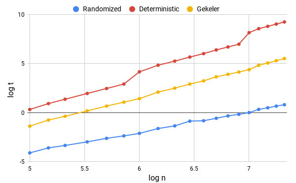
Figure 1. Log-log plot of $n$ versus runtime with $q=499$, $m=2$

- (1)
- Bostan et al. (2007) A. Bostan, P. Gaudry, and É. Schost. 2007. Linear recurrences with polynomial coefficients and application to integer factorization and Cartier-Manin operator. SIAM J. Comput. 36, 6 (2007), 1777–1806.
- Brent and Kung (1978) R. P. Brent and H. T. Kung. 1978. Fast Algorithms for Manipulating Formal Power Series. J. ACM 25, 4 (1978), 581–595.
- Carlitz (1935) L. Carlitz. 1935. On certain functions connected with polynomials in a Galois field. Duke Math. J. 1, 2 (1935), 137–168.
- Caruso and Borgne (2017) X. Caruso and J. Le Borgne. 2017. Fast multiplication for skew polynomials. In ISSAC’17. ACM, 77–84.
- Coppersmith (1994) D. Coppersmith. 1994. Solving homogeneous linear equations over GF via block Wiedemann algorithm. Math. Comp. 62, 205 (1994), 333–350.
- Coppersmith and Winograd (1990) D. Coppersmith and S. Winograd. 1990. Matrix multiplication via arithmetic progressions. J. Symb. Comput. 9, 3 (1990), 251–280.
- Doliskani et al. (2017) J. Doliskani, A. K. Narayanan, and É. Schost. 2017. Drinfeld modules with complex multiplication, Hasse invariants and factoring polynomials over finite fields. arXiv:1712.00669
- Drinfel’d (1974) V. G. Drinfel’d. 1974. Elliptic modules. Matematicheskii Sbornik 94, 23 (1974), 561–593.
- Garai and Papikian (2018) S. Garai and M. Papikian. 2018. Endomorphism rings of reductions of Drinfeld modules. arXiv:1804.07904
- Gathen and Gerhard (2013) J. von zur Gathen and J. Gerhard. 2013. Modern Computer Algebra (3 ed.). Cambridge University Press, New York, NY, USA.
- Gathen and Shoup (1992) J. von zur Gathen and V. Shoup. 1992. Computing Frobenius maps and factoring polynomials. Computational Complexity 2, 3 (1992), 187–224.
- Gekeler (1991) E.-U. Gekeler. 1991. On finite Drinfeld modules. Journal of Algebra 141, 1 (1991), 187 – 203.
- Gekeler (2008) E.-U. Gekeler. 2008. Frobenius distributions of Drinfeld modules over finite fields. Trans. Amer. Math. Soc. 360 (04 2008), 1695–1721.
- Giorgi et al. (2003) P. Giorgi, C.-P. Jeannerod, and G. Villard. 2003. On the complexity of polynomial matrix computations. In ISSAC’03. ACM, 135–142.
- Goss (1996) D. Goss. 1996. Basic Structures of Function Field Arithmetic. Springer Berlin Heidelberg.
- Harvey (2014) David Harvey. 2014. Counting points on hyperelliptic curves in average polynomial time. Annals of Mathematics 179, 2 (2014), 783–803.
- Hsia and Yu (2000) L.-C. Hsia and J. Yu. 2000. On characteristic polynomials of geometric Frobenius associated to Drinfeld modules. Compositio Mathematica 122, 3 (2000), 261–280.
- Jung (2000) F. Jung. 2000. Charakteristische Polynome von Drinfeld-Moduln. Diplomarbeit, U. Saarbrücken.
- Kaltofen and Pan (1991) E. Kaltofen and V. Pan. 1991. Processor efficient parallel solution of linear systems over an abstract field. In SPAA ’91. ACM, 180–191.
- Kaltofen and Saunders (1991) E. Kaltofen and B. D. Saunders. 1991. On Wiedemann’s method of solving sparse linear systems. In AAECC-9. Springer-Verlag, 29–38.
- Kaltofen and Shoup (1998) E. Kaltofen and V. Shoup. 1998. Subquadratic-time factoring of polynomials over finite fields. Math. Comp. 67, 223 (1998), 1179–1197.
- Kaltofen and Villard (2004) E. Kaltofen and G. Villard. 2004. On the complexity of computing determinants. Computational Complexity 13, 3-4 (2004), 91–130.
- Kaminski et al. (1988) M. Kaminski, D.G. Kirkpatrick, and N.H. Bshouty. 1988. Addition requirements for matrix and transposed matrix products. J. Algorithms 9, 3 (1988), 354–364.
- Kedlaya and Umans (2011) K. S. Kedlaya and C. Umans. 2011. Fast polynomial factorization and modular composition. SIAM J. Comput. 40, 6 (2011), 1767–1802.
- Labahn et al. (2017) G. Labahn, V. Neiger, and W. Zhou. 2017. Fast, deterministic computation of the Hermite normal form and determinant of a polynomial matrix. J. Complexity 42 (2017), 44–71.
- Le Gall (2014) F. Le Gall. 2014. Powers of tensors and fast matrix multiplication. In ISSAC’14. ACM, 296–303.
- Le Gall and Urrutia (2018) F. Le Gall and F. Urrutia. 2018. Improved rectangular matrix multiplication using powers of the Coppersmith-Winograd tensor. In SODA ’18. SIAM, 1029–1046.
- Musleh, Yossef (2018) Musleh, Yossef. 2018. Fast Algorithms for Finding the Characteristic Polynomial of a Rank-2 Drinfeld Module. http://hdl.handle.net/10012/13889
- Narayanan (2018) A. K. Narayanan. 2018. Polynomial factorization over finite fields by computing Euler-Poincaré characteristics of Drinfeld modules. Finite Fields Appl. 54 (2018), 335–365.
- Panchishkin and Potemine (1989) A. Panchishkin and I Potemine. 1989. An algorithm for the factorization of polynomials using elliptic modules. In Constructive methods and algorithms in number theory. 117.
- Pohst and Zassenhaus (1989) M. Pohst and H. Zassenhaus (Eds.). 1989. Algorithmic Algebraic Number Theory. Cambridge University Press.
- Puchinger and Wachter-Zeh (2017) S. Puchinger and A. Wachter-Zeh. 2017. Fast operations on linearized polynomials and their applications in coding theory. J. Symb. Comput. (2017).
- Satoh (2000) T Satoh. 2000. The canonical lift of an ordinary elliptic curve over a finite field and its point counting. J. Ramanujan Math. Soc. 15 (2000), 247–270.
- Scanlon (2001) T. Scanlon. 2001. Public Key cryptosystems based on Drinfeld modules Are insecure. Journal of Cryptology 14, 4 (2001), 225–230.
- Schoof (1985) R. Schoof. 1985. Elliptic curves over finite fields and the computation of square roots . Math. Comp. 44, 170 (1985), 483–494.
- Shoup (1994) V. Shoup. 1994. Fast construction of irreducible polynomials over finite fields. J. Symb. Comput. 17, 5 (1994), 371–391.
- Shoup (2019) V. Shoup. 2019. NTL: A library for doing number theory. http:/www.shoup.net/ntl.
- van der Heiden (2004) G. J. van der Heiden. 2004. Factoring polynomials over finite fields with Drinfeld modules. Math. Comp. 73 (2004), 317–322.
- Wiedemann (1986) D H Wiedemann. 1986. Solving Sparse Linear Equations over Finite Fields. IEEE Trans. Inf. Theor. 32, 1 (1986), 54–62.