Definitions of local density in density-dependent potentials for mixtures

Abstract

Density-dependent potentials are frequently used in materials simulations due to their approximate description of many-body effects at minimal computational cost. However, in order to apply such models to multi-component systems, an appropriate definition of total local particle density is required. Here, we discuss two definitions of local density in the context of many-body dissipative particle dynamics. We show that only a potential which combines local densities from all particle types in its argument gives physically meaningful results for all composition ratios. Drawing on the ideas from metal potentials, we redefine local density such that it can accommodate different inter-type interactions despite the constraint to keep the main interaction parameter constant, known as Warren’s no-go theorem, and generalise the many-body potential to heterogeneous systems. We then show via simulation how liquid-liquid and liquid-solid coexistence can arise just by tuning the interaction parameters.

I Introduction

Coarse-graining is a widely used approach across all scales to eliminate fast or unimportant degrees of freedom, speed up simulations and understand the most relevant physics. In electronic structure theory, core electrons are often coarse-grained into pseudopotentials; in classical atomistic simulations, all electrons are reduced to effective potentials between atoms; in soft matter, whole atoms and molecules can be collapsed into particles. These “blobs” interact via effective pair potentials, which differ from classical, all-atom pair potentials in that they are parametrised only for a specific thermodynamic state. Thus, these potentials do not necessarily reproduce material properties at temperatures or pressures other than the one for which they were defined, which is commonly known as the transferability problem.

A dependence on the local density (LD) of particles can be added to increase predictive abilities, motivated by the observation that some material properties cannot be captured purely by pair potentials Louis (2002); Merabia and Pagonabarraga (2007). In the solid state, LD is used to improve the description of metals and alloys. Coarse-graining electrons into an effective local electronic density significantly improves the description of fracture and the role of impurities. Examples of such metal potentials are the embedded atom method Daw and Baskes (1983, 1984), Finnis-Sinclair model Finnis and Sinclair (1984) or Sutton-Chen potential Sutton and Chen (1990).

The general form of the energy in these metal potentials is:

$$U=\sum_{i<j}V(r_{ij})+\sum_{i}u(\bar{\rho}_{i}),$$ (1)

where $u(\bar{\rho}_{i})$ is the self-energy of $i$th atom embedded in a local density $\bar{\rho}_{i}$ and $r_{ij}=|\mathbf{r}_{i}-\mathbf{r}_{j}|$ is the distance between the $i$th and $j$th atom at positions $\mathbf{r}_{i}$ and $\mathbf{r}_{j}$, respectively. The local density accounts for neighbouring particles via weight functions $w_{\mathrm{\rho}}$ which decrease with distance:

$$\bar{\rho}_{i}=\sum_{j\neq i}w_{\mathrm{\rho}}(r_{ij}).$$ (2)

For the Finnis-Sinclair and Sutton-Chen potentials, $u(\bar{\rho}_{i})=-A\sqrt{\bar{\rho}_{i}}$, where the square root is motivated by the tight binding approximation. The force on $i$th atom is:

$$\mathbf{F}_{i}=-\frac{\partial{U}}{\partial{\mathbf{r}_{i}}}=-\sum_{j}\frac{\partial{U}}{\partial{r}_{ij}}\hat{\mathbf{r}}_{ij},$$ (3)

where $\hat{\mathbf{r}}_{ij}=(\mathbf{r}_{i}-\mathbf{r}_{j})/r_{ij}$ is a unit vector.

In soft matter, potentials with LD terms have been used either with a form defined a priori in many-body dissipative particle dynamics (MDPD), or coarse-grained from the bottom-up, as with an application to mixing of water and benzene Sanyal and Shell (2016, 2018). Building on standard dissipative particle dynamics (DPD) Español and Warren (2017), MDPD is suitable for describing mesoscale systems with heterogeneous densities. This force field was introduced by Pagonabarraga and Frenkel Pagonabarraga and Frenkel (2001) in general terms as a potential for non-ideal fluids and further developed by Trofimov et al. Trofimov et al. (2002) and Warren Warren (2001, 2003). MDPD was recently parametrised by the present authors for solvent mixtures Vanya et al. (2018).

In the past decades, a significant body of research has been generated by applying standard or many-body DPD. The Karniadakis group investigated a range of applications including blood Chang et al. (2016); Li et al. (2014); Peng et al. (2013), block copolymers Li et al. (2009) and membranes Li et al. (2012). Ghoufi and Malfreyt explored extensively the vapour-liquid coexistence in MDPD Ghoufi and Malfreyt (2010, 2011); Ghoufi et al. (2013). Merabia et al. investigated wetting of liquid on a solid substrate with a model similar to the present definition of MDPD Merabia and Pagonabarraga (2006); Merabia et al. (2008); Merabia and Avalos (2008). Another, related branch of research is smoothed-particle hydrodynamics accounting for thermal fluctuations and transport by discretising the Navier-Stokes equations Español and Revenga (2003); Thieulot et al. (2005a, b); Litvinov et al. (2008).

Standard DPD has a purely repulsive pair potential with a cutoff yielding a force between two coarse-grained particles of the form:

$$\mathbf{F}_{ij}=Aw(r_{ij})\hat{\mathbf{r}}_{ij},$$ (4)

where $A$ is an interaction parameter and $w(r)$ a weight function with a linear taper: $w(r)=1-r/r_{\mathrm{c}}$ for $r<r_{\mathrm{c}}$ and 0 elsewhere. Together with the many-body term with self-energy $u(\bar{\rho})$, it can be shown via eq. (3) that the force from the MDPD potential is:

$$\mathbf{F}_{ij}=Aw(r_{ij})\hat{\mathbf{r}}_{ij}-[u^{\prime}(\bar{\rho}_{i})+u^{\prime}(\bar{\rho}_{j})]w_{\mathrm{\rho}}^{\prime}(r_{ij})\hat{\mathbf{r}}_{ij}.$$ (5)

This weight function has a cutoff and is normalised, such that $\int 4\pi r^{2}w_{\mathrm{\rho}}(r)dr=1$.

The simplest form of self-energy is $u(r_{i})=B\bar{\rho}_{i}^{2}/2$, with an interaction parameter $B$ and $w_{\mathrm{\rho}}(r)\sim(1-r/r_{\mathrm{d}})^{2}$ for $r<r_{\mathrm{d}}$ and 0 elsewhere . Setting $A<0$, $B>0$ and the many-body cutoff $r_{\mathrm{d}}<r_{\mathrm{c}}$ results in a potential that can produce a liquid-vapour coexistence, which makes MDPD applicable to systems containing interfaces between different phases.

I.1 Multicomponent systems

The generalisation of self-energy in MDPD to multicomponent systems has so far been ambiguous; the form of the LD proposed in the literature has been assumed without justification of the reasoning. For the $i$th particle, single-component LDs can be defined separately by particle type $\alpha$:

$$\bar{\rho}_{i}^{(\alpha)}=\sum_{j,j\in\alpha}w_{\mathrm{\rho}}(r_{ij}).$$ (6)

So, for $n$-component systems there are $n$ different LDs for each particle. The ambiguity lies in the fact that it is not a priori clear how to combine these correctly in the self-energy.

Mathematically, for pair potentials the energy per particle is a straightforward function of the coordinates of the neighbouring particles: $u(\{\mathbf{r}_{i}\})$. LD potentials have a function representing the LD and an outside wrapping function $u$: $u[\bar{\rho}(\{\mathbf{r}_{i}\})]$. In case of multicomponent systems, such as liquid mixtures or alloys, a question arises how to combine the terms within the wrapping function $u(x)$. Taking the simplest, two-component system composed of types $\alpha$ and $\beta$, two options are immediately apparent: (i.) $u[\bar{\rho}^{(\alpha)}(\{\mathbf{r}_{i}\})+\bar{\rho}^{(\beta)}(\{\mathbf{r}_{i}\})]$, and (ii.) $u[\bar{\rho}^{(\alpha)}(\{\mathbf{r}_{i}\})]+u[\bar{\rho}^{(\beta)}(\{\mathbf{r}_{i}\})]$ . We denote these as the partial and full LD variants respectively.

The partial LD variant was used by Sanyal et al. Sanyal and Shell (2018) and also had originally been implemented in the DL_MESO package Seaton et al. (2013), which has inspired the present exploration. The total LD variant was discussed in Section V in Trofimov et al. Trofimov et al. (2002) and, implicitly, in Warren Warren (2013), when introducing the no-go theorem stating that the parameter $B$ must be constant across particle types if the potential $U$ is to be conservative.

In this work, we discuss the viability of these two LD variants of multicomponent systems. We show that the partial variant can have type-dependent parameters $B^{(\alpha\beta)}$, but it behaves unphysically in that a simple relabelling of particles alters the forces between them. This in turn affects local ordering and phase behaviour. As a result, only the total LD variant is usable in practice. Drawing on research in solid state physics, we redefine the latter such that it can accommodate variability among different particle types.

To illustrate these points, we take a minimal two-component mixture of three particles and explicitly compute the forces between them for each of the variants of local density (Fig. 1). We work with a general form of self-energy $u(\bar{\rho}_{i})$ and weight function $w_{\mathrm{\rho}}(r)$ and assume that all the particles are within the cutoff distance of one another. This reasoning also applies to other density-dependent potentials, not just MDPD.

To proceed with algebra, we first define the necessary notation. In the most general case, there are three different interaction parameters in a two-component system. Like particles of type $\alpha$ and $\beta$ interact via parameters $B^{(\alpha\alpha)}$ and $B^{(\beta\beta)}$, respectively, and unlike particles via $B^{(\alpha\beta)}$. To treat the interaction parameter $B$ as an explicit prefactor, as in the case of metal potentials, we introduce a wrapping function $\psi$ such that $u(\bar{\rho}_{i})=B\psi(\bar{\rho}_{i})$. Commonly, $\psi(\bar{\rho})$ is a polynomial, $\psi=\bar{\rho}^{n}/n$, with $n=2$ in MDPD.

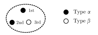
Figure 1: A minimal multicomponent system to explore local density potentials.

Particle	Partial, type $\alpha$	Partial, type $\beta$	Total
1	$\bar{\rho}^{(\alpha)}_{1}=w_{\mathrm{\rho}}(r_{12})$	$\bar{\rho}^{(\beta)}_{1}=w_{\mathrm{\rho}}(r_{13})$	$\bar{\rho}_{1}=w_{\mathrm{\rho}}(r_{12})+w_{\mathrm{\rho}}(r_{13})$
2	$\bar{\rho}^{(\alpha)}_{2}=w_{\mathrm{\rho}}(r_{12})$	$\bar{\rho}^{(\beta)}_{2}=w_{\mathrm{\rho}}(r_{23})$	$\bar{\rho}_{2}=w_{\mathrm{\rho}}(r_{12})+w_{\mathrm{\rho}}(r_{23})$
3	$\bar{\rho}^{(\alpha)}_{3}=w_{\mathrm{\rho}}(r_{13})+w_{\mathrm{\rho}}(r_{23})$	$\bar{\rho}^{(\beta)}_{3}=0$	$\bar{\rho}_{3}=w_{\mathrm{\rho}}(r_{13})+w_{\mathrm{\rho}}(r_{23})$

Table 1: List of partial local densities for each particle.

II Derivation of forces for partial local densities

Starting with the partial LD variant, the local densities can be listed explicitly (Table 1) for each of the three particles in the minimal system. From these, the self-energies of the particles follow:

$$u_{1} =B^{(\alpha\alpha)}\psi(\bar{\rho}^{(\alpha)}_{1})+B^{(\alpha\beta)}\psi(\bar{\rho}^{(\beta)}_{1}),$$ (7)

$$u_{2} =B^{(\alpha\alpha)}\psi(\bar{\rho}^{(\alpha)}_{2})+B^{(\alpha\beta)}\psi(\bar{\rho}^{(\beta)}_{2}),$$ (8)

$$u_{3} =B^{(\alpha\beta)}\psi(\bar{\rho}^{(\alpha)}_{3})+B^{(\beta\beta)}\psi(\bar{\rho}^{(\beta)}_{3}).$$ (9)

The total energy $U=u_{1}+u_{2}+u_{3}$. Computing, e.g., $\partial{U}/\partial{\mathbf{r}_{1}}$:

$$\frac{\partial{U}}{\partial{\mathbf{r}_{1}}}=B^{(\alpha\alpha)}[\psi^{\prime}(\bar{\rho}^{(\alpha)}_{1})+\psi^{\prime}(\bar{\rho}^{(\alpha)}_{2})]w_{\mathrm{\rho}}^{\prime}(r_{12})\hat{\mathbf{r}}_{12}\\ +B^{(\alpha\beta)}[\psi^{\prime}(\bar{\rho}^{(\beta)}_{1})+\psi^{\prime}(\bar{\rho}^{(\alpha)}_{3})]w_{\mathrm{\rho}}^{\prime}(r_{13})\hat{\mathbf{r}}_{13},$$ (10)

$\partial{U}/\partial{\mathbf{r}_{2}}$ can be obtained from eq. (10) by simply transposing particle indices 1 and 2 and:

$$\frac{\partial{U}}{\partial{\mathbf{r}_{3}}}=B^{(\alpha\beta)}[\psi(\bar{\rho}^{(\beta)}_{1})+\psi^{\prime}(\bar{\rho}^{(\alpha)}_{3})]w_{\mathrm{\rho}}^{\prime}(r_{12})\hat{\mathbf{r}}_{31}\\ +B^{(\alpha\beta)}[\psi^{\prime}(\bar{\rho}^{(\beta)}_{2})+\psi(\bar{\rho}^{(\alpha)}_{3})]w_{\mathrm{\rho}}^{\prime}(r_{23})\hat{\mathbf{r}}_{32}.$$ (11)

Every force $\mathbf{F}_{ij}$ has the form of eq. (3) and $\mathbf{F}_{ij}=-\mathbf{F}_{ji}$ for every pair $\{i,j\}$ in line with Newton’s third law. Hence, the self-energy of the partial LD variant is conservative and, at the same time, allows for type-specific interaction parameters $B$.

III Problem with particle relabelling

The freedom to use different parameters for unlike types provided by the partial LD variant can be important for an appropriate depiction of phase behaviour of mixtures. However, a new problem arises: the interaction strength of particles of unlike types is artificially lowered only due to the fact that they have different labels, not due to physical differences.

In a homogeneous, single-component MDPD liquid with parameter $B$, the local density is same for every particle and equal to the global density, $\bar{\rho}_{i}\approx\rho$ (assuming mean-field approximation). The force between any two particles is then:

$$\mathbf{F}_{ij} \approx B[\psi^{\prime}(\rho)+\psi^{\prime}(\rho)]w_{\mathrm{\rho}}^{\prime}(r_{ij})\hat{\mathbf{r}}_{ij}$$

$$=2B\psi^{\prime}(\rho)w_{\mathrm{\rho}}^{\prime}(r_{ij})\hat{\mathbf{r}}_{ij}.$$ (12)

Consider randomly splitting all the particles into two types but keeping the interaction parameter constant, $B^{(\alpha\alpha)}=B^{(\alpha\beta)}=B^{(\beta\beta)}=B$. Now, every particle sees around itself, on average, one half of the particles of type $\alpha$ and the other half of type $\beta$, as the system remains physically the same and hence perfectly mixed. Therefore, the average local density of both type $\alpha$ and $\beta$ particles is $\bar{\rho}_{i}^{(\alpha/\beta)}\approx\rho/2$. Computing the force between like type particles $i$ and $j$ yields:

$$\mathbf{F}_{ij} =B[\psi^{\prime}(\rho/2)+\psi^{\prime}(\rho/2)]w_{\mathrm{\rho}}^{\prime}(r_{ij})\hat{\mathbf{r}}_{ij}$$

$$=2B\psi^{\prime}(\rho/2)w_{\mathrm{\rho}}^{\prime}(r_{ij})\hat{\mathbf{r}}_{ij}.$$ (13)

These forces are not equal, since generally $\psi^{\prime}(\rho)\neq\psi^{\prime}(\rho/2)$. The only exception is the case when $\psi$ depends linearly on $\bar{\rho}$ and $\psi^{\prime}\sim 1$, which is the force field of standard DPD. With the simplest non-trivial definition of self-energy, $\psi(\bar{\rho})=\bar{\rho}^{2}/2$, the force on any particle would become twice as small purely due to relabelling, and, in simulations of mixtures with $m\gg 1$ components, $m$-times smaller.

This flaw is manifest in the local structure of a liquid, which is represented by the radial distribution function (RDF). Using DL_MESO version 2.6 Seaton et al. (2013), we set up two simulations of an effectively single-component liquid with arbitrarily relabelled particles, exploring the full LD variant with parameter $B=10$ and partial LD variant with $B=20$, which should be different liquids. In each case we measured $g^{(\alpha\beta)}(r)$. Fig. 2 shows the near identity of these two RDFs, demonstrating that the partial LD variant artificially lowers the interaction by a factor of two.

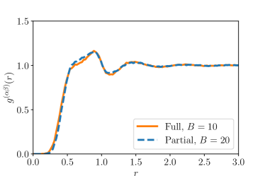
Figure 2: Inter-type radial distribution functions of two variants of local density demonstrating the unphysical behaviour of the partial variant. The slight deviation is most likely due to the different temperatures at which these systems equilibrate.

To illustrate the practical consequences of this, we consider a binary liquid interacting via an MDPD potential where interaction parameters are constant across particle types, $A=-18$ and $B=8$. These values represent water at a coarse-graining degree 6 with equilibrium density $\rho_{0}=6.70$ Vanya et al. (2019). Setting the density to $\rho=7>\rho_{0}$, this effectively single-component liquid with arbitrarily relabelled particles should homogeneously fill the simulation cell. We simulated the two local density variants and composed density profiles for each type after equilibration. Fig. 3 shows that the expected phase behaviour for a homogeneous liquid is only reproduced with the total LD variant.

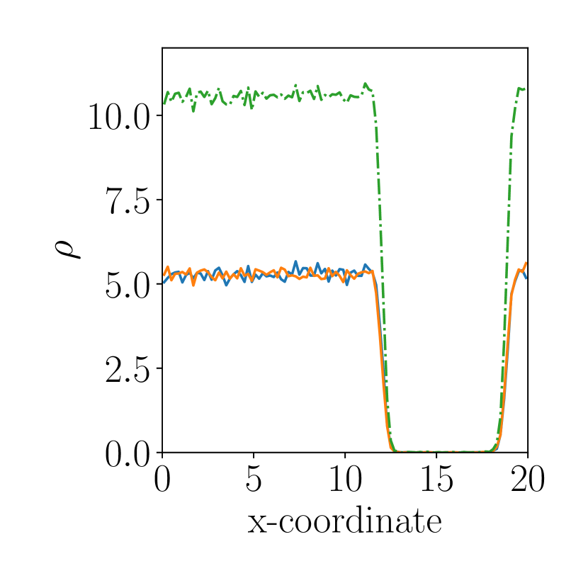
(a)

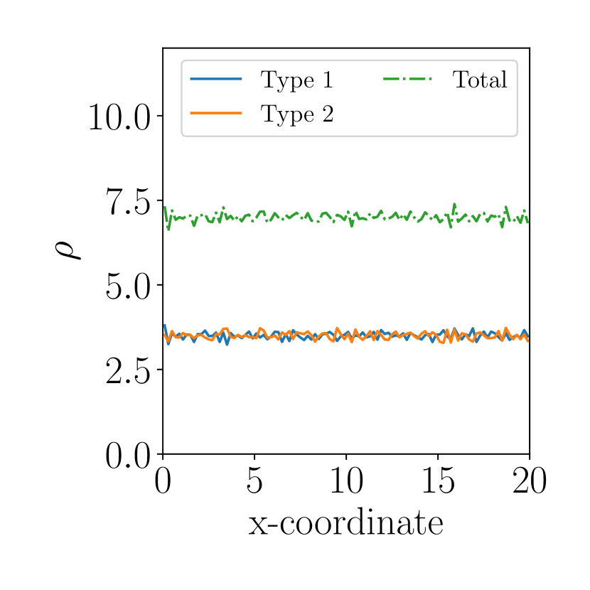
(b)

Figure 3: Density profiles of a homogeneous liquid with particles randomly split into two types, for (a) partial and (b) total local density variant. The former produces an unphysically high global density and a spurious vapour phase. The values of $\rho$ and $x$ are given in DPD units.

IV Generalised many-body force field

IV.1 Derivation of forces for total local densities

Having shown that the partial LD variant produces unphysical behaviour, only the total LD variant, which works with $\bar{\rho}_{i}=\bar{\rho}^{(\alpha)}_{i}+\bar{\rho}^{(\beta)}_{i}$, remains. However, Warren’s no-go theorem states that, for a type-independent definition of local density (eq. (6)), only a type-independent parameter $B$ is allowed, i.e. $u_{i}=B\psi(\bar{\rho}_{i})$ $\forall i$ Warren (2013). This means that the self-energy for the force on, e.g., 1st particle with the following form:

$$\mathbf{F}_{1}=-B^{(\alpha\alpha)}(\psi^{\prime}(\bar{\rho}_{1})+\psi^{\prime}(\bar{\rho}_{2}))w_{\mathrm{\rho}}^{\prime}(r_{12})\hat{\mathbf{r}}_{12}\\ -B^{(\alpha\beta)}(\psi^{\prime}(\bar{\rho}_{1})+\psi^{\prime}(\bar{\rho}_{3}))w_{\mathrm{\rho}}^{\prime}(r_{13})\hat{\mathbf{r}}_{13}.$$ (14)

does not exist unless $B^{(\alpha\alpha)}=B^{(\alpha\beta)}=B^{(\beta\beta)}$. This constraint on $B$ means that it is not possible to distinguish particles in MDPD purely by the many-body potential term, which limits the versatility of this method.

Borrowing from the formalism of metal potentials, we show that there is a way to preserve type-dependent forces by introducing a type-dependent local density Rafii-Tabar and Sulton (1991); Johnson (1989). Generally the local density for particle of type $\alpha$ accounting for neighbouring particles of type $\beta$ is:

$$\bar{\rho}^{(\alpha\beta)}_{i}=\sum_{j}w_{\mathrm{\rho}}^{(\alpha\beta)}(r_{ij}),\quad i\in\alpha,\quad j\in\beta.$$ (15)

For a two-component system, there are four possible local densities: $\bar{\rho}^{(\alpha\alpha)},\bar{\rho}^{(\alpha\beta)},\bar{\rho}^{(\beta\alpha)},\bar{\rho}^{(\beta\beta)}$. Generally, the influence of a particle of type $\alpha$ to the local density of a particle of type $\beta$ might not be the same, but in practice $\bar{\rho}^{(\alpha\beta)}=\bar{\rho}^{(\beta\alpha)}$.

Considering again the minimal three-particle system (Fig. 1), the self-energies are:

$$u_{1} =B\psi\left(\bar{\rho}_{1}^{(\alpha\alpha)}+\bar{\rho}_{1}^{(\alpha\beta)}\right)=B\psi(\bar{\rho}_{1}),$$ (16)

$$u_{2} =B\psi\left(\bar{\rho}_{2}^{(\alpha\alpha)}+\bar{\rho}_{2}^{(\alpha\beta)}\right)=B\psi(\bar{\rho}_{2}),$$ (17)

$$u_{3} =B\psi\left(\bar{\rho}_{3}^{(\alpha\beta)}+\bar{\rho}_{3}^{(\beta\beta)}\right)=B\psi(\bar{\rho}_{3}),$$ (18)

and the total energy $U=u_{1}+u_{2}+u_{3}$. Differentiating to obtain the force on particle 1 yields:

$$\mathbf{F}_{1}=-B[\psi^{\prime}(\bar{\rho}_{1})+\psi^{\prime}(\bar{\rho}_{2})]w_{\mathrm{\rho}}^{\prime(\alpha\alpha)}(r_{12})\hat{\mathbf{r}}_{12}\\ -B[\psi^{\prime}(\bar{\rho}_{1})+\psi^{\prime}(\bar{\rho}_{3})]w_{\mathrm{\rho}}^{\prime(\alpha\beta)}(r_{13})\hat{\mathbf{r}}_{13}\\ =-\mathbf{F}_{12}-\mathbf{F}_{13},$$ (19)

and the forces on forces on particles 2 and 3 can be obtained similarly.

The cross-type interaction is now represented by the term $Bw_{\mathrm{\rho}}^{\prime(\alpha\beta)}$, which gives the freedom to tune it via the derivative of the weight function $w_{\mathrm{\rho}}^{(\alpha\beta)}$. A simple arithmetic mixing rule can be used: $w_{\mathrm{\rho}}^{(\alpha\beta)}=\left(w_{\mathrm{\rho}}^{(\alpha\alpha)}+w_{\mathrm{\rho}}^{(\beta\beta)}\right)/2$, but a more general form might be required for coarse-grained systems, possibly involving the Flory-Huggins $\chi$-parameter as in the case of standard DPD. (A geometric mixing, as in the case of metal potentials Rafii-Tabar and Sulton (1991), might not be suitable due to the explicit and necessary cutoff of coarse-grained potentials.)

IV.2 Mixing of different material types

Finally, we address the mixing of different materials. An example is a liquid or a polymer on metal surface, which is a typical setting for heterogeneous catalysis and so is of immense practical importance.

The total LD self-energy allows for definitions of the wrapping function $\psi$ depending on the material phase. Referring to Fig. 1, consider the first two particles metallic (M) and the third a liquid (L). Each phase has a different wrapping function: $\psi_{\rm M}$ for a metal can be a square root, and $\psi_{\rm L}$ for a liquid can be a square to allow for liquid-vapour coexistence. The self-energies are:

$$u_{1} =B\psi_{\rm M}\left(\bar{\rho}_{1}^{(\alpha\alpha)}+\bar{\rho}_{1}^{(\alpha\beta)}\right)=B\psi_{\rm M}(\bar{\rho}_{1}),$$ (20)

$$u_{2} =B\psi_{\rm M}\left(\bar{\rho}_{2}^{(\alpha\alpha)}+\bar{\rho}_{2}^{(\alpha\beta)}\right)=B\psi_{\rm M}(\bar{\rho}_{2}),$$ (21)

$$u_{3} =B\psi_{\rm L}\left(\bar{\rho}_{3}^{(\alpha\beta)}+\bar{\rho}_{3}^{(\beta\beta)}\right)=B\psi_{\rm L}(\bar{\rho}_{3}).$$ (22)

Following the previous section, the force on particle 1 is:

$$\mathbf{F}_{1}=-B[\psi_{\rm M}^{\prime}(\bar{\rho}_{1})+\psi_{\rm M}^{\prime}(\bar{\rho}_{2})]w_{\mathrm{\rho}}^{\prime(\alpha\alpha)}(r_{12})\hat{\mathbf{r}}_{12}\\ -B[\psi_{\rm M}^{\prime}(\bar{\rho}_{1})+\psi_{\rm L}^{\prime}(\bar{\rho}_{3})]w_{\mathrm{\rho}}^{\prime(\alpha\beta)}(r_{13})\hat{\mathbf{r}}_{13},$$ (23)

where $\mathbf{F}_{13}$ contains one term from neighbouring metal atoms, $\psi^{\prime}_{\rm M}$, and another from neighbouring liquid particles, $\psi^{\prime}_{\rm L}$. The cross-type weight function $w_{\mathrm{\rho}}^{(\alpha\beta)}$ requires further investigation to determine its appropriate form or a range of forms, but at this stage it is sufficient to note that, as before, it represents unambiguously the material-dependent interaction via the term $Bw_{\mathrm{\rho}}^{\prime(\alpha\beta)}$.

IV.3 Exploring new force fields via simulation

To demonstrate the versatility of this generalised MDPD force field for describing inhomogeneous mixtures, we perform several simulations using a custom-written code .

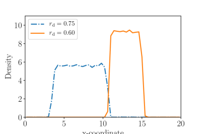
Figure 4: A coexistence of inhomogeneous liquids using a generalised MDPD force field allowing for different many-body cutoffs.

Before doing so, it is necessary to redefine the repulsion parameter $B$ to follow the logic of the embedded atom method using unique $B$’s but varying parameters within the wrapping functions with particle type. The convention with MDPD has been so far to define $B$ through the force: $F_{ij}=B_{\rm o}(\bar{\rho}_{i}+\bar{\rho}_{j})(1-r/r_{\mathrm{d}})$ with $r<r_{\mathrm{d}}$ Warren (2003). Here, we start from the energy, $u_{i}=B\bar{\rho}_{i}^{2}/2$, so $B$ is modified by the normalisation factor of the weight function; the force for like-type particles then becomes $F_{ij}=15/(\pi r_{\mathrm{d}}^{4})\,B\,(\bar{\rho}_{i}+\bar{\rho}_{j})(1-r/r_{\mathrm{d}})$, so $B=B_{\rm o}\,\pi r_{\mathrm{d}}^{4}/15$. For a typical value of $B_{\rm o}=30$, $B\approx 2$ for $r_{\mathrm{d}}=0.75$.

Using this convention, we first investigate inhomogeneous liquids with same quadratic wrapping function for both particle types, $\psi(x)=x^{2}/2$, with parameters $A=-40,B=2$. The cross-type repulsion is represented by decreased attraction $A_{12}=A+\Delta A$, setting $\Delta A=20$. The difference between the liquids is marked by many-body cutoff set to 0.75 and 0.60 for type 1 and type 2, respectively, and cross-interaction as the arithmetic mean of these, 0.675. The simulation contained 2000 particles, split equally between the two types, in a $20\times 5\times 5$ cell and was run for 200 reduced time units with timestep $\Delta t=0.01$. Figure 4 shows a coexistence of two separated phases at different densities, a feature so far unavailable in MDPD.

As a second simulation, following eq. (22) we consider a system with wrapping functions differing with particle types. For simplicity, we constrain the choice to polynomial functions: $\psi(x)=x^{N_{\mathrm{w}}}/N_{\mathrm{w}}$. We chose $N_{\mathrm{w}}=2$ for phase 1 and $N_{\mathrm{w}}=3$ for phase 2, the repulsion parameter $B=3$, and many-body cutoffs $r_{\mathrm{d}}^{(11)}=0.75$, $r_{\mathrm{d}}^{(22)}=0.55$, and $r_{\mathrm{d}}^{(12)}=0.65$. We simulated for the same time period as before using a smaller timestep, $\Delta t=0.006$ in order to retain the temperature within 10% of $k_{\rm B}T=1$. This setup shows the coexistence of a liquid and a solid phase (Fig. 5). The solid phase is identified by a radial distribution function with a sharp first peak and more frequent oscillations, in contrast to that for the liquid phase, which is flatter and smoother (in the inset of Fig. 5). This can be compared with Fig. 5a of our previous work Vanya et al. (2018).

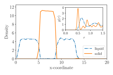
Figure 5: A coexistence of liquid and solid phase using a generalised MDPD force field achieved by choosing different many-body cutoffs and wrapping functions. The inset shows radial distribution functions; the tall first peak of the orange curve is a signature of the solid phase.

With these exploratory simulations, we note several observations. Firstly, is not advisable to use $N_{\mathrm{w}}=1/2$, as in the embedded atom method, due to the finiteness of the MDPD potential. This feature produces, with some non-negligible probability, vanishing local densities, from which, after taking the derivative to compute forces, results in a zero in the denominator. A solution could be to increase the range, but this would go against the spirit of coarse-graining and simulation efficiency. Secondly, with increasing $N_{\mathrm{w}}$ it is necessary to minimise the box prior to the simulation run; such a need does not arise with lower values due to fast equilibration. Thirdly, it is also possible to achieve a liquid-solid phase coexistence using purely $N_{\mathrm{w}}=2$ for both particle types and controlling the difference between the phases only by the many-body cutoff. Fourth, we only set the cross-type repulsion via the interaction parameter $A$ and many-body cutoff $r_{\mathrm{d}}$; there are other options to modify the many-body part of the interaction apart from the parameter $r_{\mathrm{d}}$ that could provide further flexibility to describe real materials; these remain to be investigated.

Finally, there is the question of applications of the generalised MDPD force field to real materials. Standard DPD as well as many-body DPD relied on ad hoc parametrisation dependent on the choice of the material by setting the reduced length scale based on its molecular volume. However, each component of a heterogeneous mixture has its own scale, so a new parametrisation protocol must be devised. As the atomistic resolution, on which the EAM is based, is not available, and the metallic faces and lattice constants are ambiguous concepts in coarse-graining, an open question remains about what the default physical properties for the parametrisation of the solid state should be. It could be possible to use the total energy and compressibility.

V Conclusion

The definition of local density for many-body, density-dependent potentials must include all particle types. Otherwise, a mathematical relabelling of particles yields unphysical results unless the potential energy is redefined. Following the idea of alloys in metal potentials, we showed that the total local density composed of contributions from all particles can be distinguished by the particle type and is able to account for different cross-type interactions despite the need to keep the main interaction parameter constant to obey Warren’s no-go theorem Warren (2013).

We generalised the many-body coarse-grained potential and demonstrated its usefulness via simulations of a mixture of liquids with unequal densities and a liquid-solid system. This force field thus opens up avenues for treatment of material combinations such as soft matter on metal surface with potential applications in heterogeneous catalysis.

VI Acknowledgments

The authors thank Johnson Matthey and the Engineering and Physical Sciences Research Council (EPSRC) for financial support and Soňa Slobodníková for inspiring scientific discussions.

References

- Louis (2002) A. A. Louis, Journal of Physics: Condensed Matter 14, 9187 (2002).
- Merabia and Pagonabarraga (2007) S. Merabia and I. Pagonabarraga, The Journal of Chemical Physics 127, 054903 (2007).
- Daw and Baskes (1983) M. S. Daw and M. I. Baskes, Phys. Rev. Lett. 50, 1285 (1983).
- Daw and Baskes (1984) M. S. Daw and M. I. Baskes, Phys. Rev. B 29, 6443 (1984).
- Finnis and Sinclair (1984) M. W. Finnis and J. E. Sinclair, Philosophical Magazine A 50, 45 (1984).
- Sutton and Chen (1990) A. P. Sutton and J. Chen, Philosophical Magazine Letters 61, 139 (1990).
- Sanyal and Shell (2016) T. Sanyal and M. S. Shell, The Journal of Chemical Physics 145, 034109 (2016).
- Sanyal and Shell (2018) T. Sanyal and M. S. Shell, The Journal of Physical Chemistry B 122, 5678 (2018), pMID: 29466859.
- Español and Warren (2017) P. Español and P. B. Warren, The Journal of Chemical Physics 146, 150901 (2017).
- Pagonabarraga and Frenkel (2001) I. Pagonabarraga and D. Frenkel, The Journal of Chemical Physics 115, 5015 (2001).
- Trofimov et al. (2002) S. Y. Trofimov, E. L. F. Nies, and M. a. J. Michels, The Journal of Chemical Physics 117, 9383 (2002).
- Warren (2001) P. B. Warren, Phys. Rev. Lett. 87, 225702 (2001).
- Warren (2003) P. B. Warren, Phys. Rev. E 68, 066702 (2003).
- Vanya et al. (2018) P. Vanya, P. Crout, J. Sharman, and J. A. Elliott, Phys. Rev. E 98, 033310 (2018).
- Chang et al. (2016) H.-Y. Chang, X. Li, H. Li, and G. E. Karniadakis, PLOS Computational Biology 12, 1 (2016).
- Li et al. (2014) X. Li, Z. Peng, H. Lei, M. Dao, and G. E. Karniadakis, Philosophical Transactions of the Royal Society A: Mathematical, Physical and Engineering Sciences 372, 20130389 (2014).
- Peng et al. (2013) Z. Peng, X. Li, I. V. Pivkin, M. Dao, G. E. Karniadakis, and S. Suresh, Proceedings of the National Academy of Sciences 110, 13356 (2013), https://www.pnas.org/content/110/33/13356.full.pdf .
- Li et al. (2009) X. Li, I. V. Pivkin, H. Liang, and G. E. Karniadakis, Macromolecules 42, 3195 (2009).
- Li et al. (2012) Y. Li, X. Li, Z. Li, and H. Gao, Nanoscale 4, 3768 (2012).
- Ghoufi and Malfreyt (2010) A. Ghoufi and P. Malfreyt, Phys. Rev. E 82, 016706 (2010).
- Ghoufi and Malfreyt (2011) a. Ghoufi and P. Malfreyt, Physical Review E - Statistical, Nonlinear, and Soft Matter Physics 83, 1 (2011).
- Ghoufi et al. (2013) A. Ghoufi, J. Emile, and P. Malfreyt, The European physical journal. E, Soft matter 36, 10 (2013).
- Merabia and Pagonabarraga (2006) S. Merabia and I. Pagonabarraga, The European Physical Journal E 20, 209 (2006).
- Merabia et al. (2008) S. Merabia, J. Bonet-Avalos, and I. Pagonabarraga, Journal of Non-Newtonian Fluid Mechanics 154, 13 (2008).
- Merabia and Avalos (2008) S. Merabia and J. B. Avalos, Phys. Rev. Lett. 101, 208304 (2008).
- Español and Revenga (2003) P. Español and M. Revenga, Phys. Rev. E 67, 026705 (2003).
- Thieulot et al. (2005a) C. Thieulot, L. P. B. M. Janssen, and P. Español, Phys. Rev. E 72, 016713 (2005a).
- Thieulot et al. (2005b) C. Thieulot, L. P. B. M. Janssen, and P. Español, Phys. Rev. E 72, 016714 (2005b).
- Litvinov et al. (2008) S. Litvinov, M. Ellero, X. Hu, and N. A. Adams, Phys. Rev. E 77, 066703 (2008).
- Note (1) In general, any power of the local density can be considered and thus the equation of state can be influenced, as was demonstrated by Trofimov et al. Trofimov et al. (2002).
- Note (2) There is also a trivial function where the self-energy contains only the local density of the particles of the like type, . However, the resulting force is the same as for the partial local density variant.
- Seaton et al. (2013) M. A. Seaton, R. L. Anderson, S. Metz, and W. Smith, Molecular Simulation 39, 796 (2013), http://dx.doi.org/10.1080/08927022.2013.772297 .
- Warren (2013) P. B. Warren, Phys. Rev. E 87, 045303 (2013).
- Vanya et al. (2019) P. Vanya, J. Sharman, and J. A. Elliott, The Journal of Chemical Physics 150, 064101 (2019).
- Rafii-Tabar and Sulton (1991) H. Rafii-Tabar and A. P. Sulton, Philosophical Magazine Letters 63, 217 (1991).
- Johnson (1989) R. A. Johnson, Phys. Rev. B 39, 12554 (1989).
- Note (3) Available at https://github.com/petervanya/DPDsim.