NLO QCD predictions for $\boldsymbol{t\bar{t}b\bar{b}}$ production in association with a light jet at the LHC

Abstract

Theoretical predictions for $t\bar{t}b\bar{b}$ production are of crucial importance for $t\bar{t}H$ measurements in the $H\to b\bar{b}$ channel at the LHC. To address the large uncertainties associated with the modelling of extra QCD radiation in $t\bar{t}b\bar{b}$ events, in this paper we present a calculation of $pp\to t\bar{t}b\bar{b}j$ at NLO QCD. The behaviour of NLO corrections is analysed in a variety of observables, and to assess theoretical uncertainties we use factor-two rescalings as well as different dynamic scales. In this context, we propose a systematic alignment of dynamic scales that makes it possible to disentangle normalisation and shape uncertainties in a transparent way. Scale uncertainties at NLO are typically at the level of 20–30% in integrated cross sections, and below 10% for the shapes of distributions. The kinematics of QCD radiation is investigated in detail, including the effects of its recoil on the objects of the $t\bar{t}b\bar{b}$ system. In particular, we discuss various azimuthal correlations that allow one to characterise the QCD recoil pattern in a precise and transparent way. In general, the calculation at hand provides a variety of precise benchmarks that can be used to validate the modelling of QCD radiation in $t\bar{t}b\bar{b}$ generators. Moreover, as we will argue, $pp\to t\bar{t}b\bar{b}j$ at NLO entails information that can be used to gain insights into the perturbative convergence of the inclusive $t\bar{t}b\bar{b}$ cross section beyond NLO. Based on this idea, we address the issue of the large NLO $K$-factor observed in $\sigma_{t\bar{t}b\bar{b}}$, and we provide evidence that supports the reduction of this $K$-factor through a mild adjustment of the QCD scales that are conventionally used for this process. The presented $2\to 5$ NLO calculations have been carried out using OpenLoops 2 in combination with Sherpa and Munich.

1 Introduction

The associated production of top- and bottom-quark pairs at hadron colliders is an especially interesting process. From the theoretical point of view, it offers rich opportunities to investigate the dynamics of QCD in the presence of multiple scattering particles and energy scales. In particular, higher-order calculations of $pp\to t\bar{t}b\bar{b}$ raise non-trivial questions related to the mass gap between $m_{b}$ and $m_{t}$, the choice of QCD scales, and the convergence of the perturbative expansion. Further strong motivation for a deeper understanding of $t\bar{t}b\bar{b}$ production comes from its critical role as irreducible background to $t\bar{t}H$ production with $H\to b\bar{b}$ at the LHC Aaboud:2017rss ; Sirunyan:2018mvw ; CMS:2019lcn . In this context, the modelling of $pp\to t\bar{t}b\bar{b}$ represents the main source of uncertainty in $t\bar{t}H(b\bar{b})$ measurements. Thus, improving the theoretical description of the $t\bar{t}b\bar{b}$ background is of great importance for the sensitivity of $t\bar{t}H(b\bar{b})$ analyses at the High-Luminosity LHC Cepeda:2019klc . Precise theoretical calculations for $t\bar{t}b\bar{b}$ production are relevant also for direct experimental studies of this process, and recent measurements of the $t\bar{t}b\bar{b}$ cross section Sirunyan:2017snr ; Aaboud:2018eki ; CMS:2019dij tend to exceed theory predictions by $30$–$50$%.

At leading order (LO) in QCD, the $t\bar{t}b\bar{b}$ cross section is proportional to $\alpha_{\mathrm{S}}^{4}$ and suffers from huge scale uncertainties. Next-to-leading order (NLO) QCD calculations Bredenstein:2009aj ; Bevilacqua:2009zn ; Bredenstein:2010rs reduce scale uncertainties to $20$–$30$%, but the level of precision and the size of the corrections depend in a critical way on the choice of the renormalisation scale $\mu_{\mathrm{R}}$. In this respect, in order to avoid an excessively large NLO $K$-factor, it was found that the value of $\mu_{\mathrm{R}}$ should be chosen in the vicinity of the geometric average of the energy scales of the $t\bar{t}$ and $b\bar{b}$ systems Bredenstein:2010rs .

Calculations of $pp\to t\bar{t}b\bar{b}$ based on the five-flavour (5F) scheme Bredenstein:2009aj ; Bevilacqua:2009zn ; Bredenstein:2010rs , where $b$-quarks are treated as massless partons, are applicable only to the phase space with two resolved $b$-jets, while including $b$-mass effects in the four-flavour (4F) scheme makes it possible to obtain NLO predictions in the full $t\bar{t}+b$-jets phase space Cascioli:2013era , including regions where one $b$-quark is unresolved. The choice of the 4F scheme as opposed to the 5F scheme is also supported by the fact that initial-state $g\to b\bar{b}$ splittings play a marginal role in $t\bar{t}+b$-jets production, while the vast majority of $b$-jets originate via initial-state gluon radiation with subsequent $g\to b\bar{b}$ splittings Jezo:2018yaf .

In order to be applicable to $t\bar{t}H(b\bar{b})$ measurements, NLO calculations of $pp\to t\bar{t}b\bar{b}$ need to be matched to parton showers. Nowadays, this can be achieved within various Monte Carlo frameworks Garzelli:2014aba ; Bevilacqua:2017cru; Cascioli:2013era ; Alwall:2014hca ; Jezo:2018yaf ; Bellm:2015jjp , using different matching methods and parton showers. Some of these generators are in good mutual agreement, but the overall spread of Monte Carlo predictions suggests that $t\bar{t}b\bar{b}$ modelling uncertainties may significantly exceed the level of QCD scale variations, thereby spoiling NLO accuracy deFlorian:2016spz . In this context, the uncertainties related to the modelling of extra QCD radiation that accompanies $t\bar{t}b\bar{b}$ production play a dominant role.

Motivated by these observations, in this paper we present a NLO QCD calculation of $t\bar{t}b\bar{b}$ production in association with one additional jet at the LHC. Bottom-mass effects are included throughout using the 4F scheme. For the calculation of the required $2\to 5$ one-loop amplitudes, which involve up to 25’000 diagrams in a single partonic channel, we use the latest version of the OpenLoops program Buccioni:2019sur , where scattering amplitudes are computed with the new on-the-fly reduction method presented in Buccioni:2017yxi . For the calculation of hadronic cross sections, OpenLoops 2 is interfaced with Sherpa Krauss:2001iv ; Gleisberg:2008ta ; Gleisberg:2008fv ; Gleisberg:2007md and, alternatively, with Munich.

We discuss NLO predictions for $pp\to t\bar{t}b\bar{b}j$ at 13 TeV with emphasis on the assessment of perturbative uncertainties. To this end, we study conventional scale variations as well as different dynamic scales, and we point out that the effects of these two kinds of scale uncertainties are largely correlated. Based on this observation, we propose the idea of aligning dynamic scales to a natural scale, which can be defined using the maxima of the NLO variation curves as a reference. This prescription makes it possible to disentangle the effects of factor-two variations and dynamic scale variations in a way that provides a more transparent picture of normalisation and shape uncertainties.

To characterise the behaviour of QCD radiation in $t\bar{t}b\bar{b}$ events, we consider kinematic distributions in the hardest light jet as well as recoil effects on the various objects of the $t\bar{t}b\bar{b}$ system. To this end, we introduce azimuthal angular correlations that provide a transparent and perturbatively stable picture of recoil effects. Our NLO predictions for these and various other observables can be used as precision benchmarks to validate the modelling of QCD radiation in $t\bar{t}b\bar{b}$ generators.

Finally, we exploit the calculation at hand to address the issue of the large NLO $K$-factor observed in the integrated $t\bar{t}b\bar{b}$ cross section Jezo:2018yaf . In this respect, we note that the NLO corrections to $pp\to t\bar{t}b\bar{b}j$ correspond to the same order in $\alpha_{\mathrm{S}}$ as the NNLO corrections to inclusive $t\bar{t}b\bar{b}$ production, i.e. $\mathcal{O}(\alpha_{\mathrm{S}}^{6})$. Thus they entail (partial) information on the behaviour of $\sigma_{t\bar{t}b\bar{b}}$ beyond NLO. Based on this idea, we use the $t\bar{t}b\bar{b}j$ cross section at NLO to identify an optimal scale choice for the process $pp\to t\bar{t}b\bar{b}$. The results of this analysis support a slight adjustment of the conventional $t\bar{t}b\bar{b}$ scale choice, which results in a reduction of the $t\bar{t}b\bar{b}$ $K$-factor and is also expected to attenuate NLO matching uncertainties.

The paper is organised as follows. In Sections 2–3 we outline the main ingredients of $pp\to t\bar{t}b\bar{b}j$ at NLO, and we document the employed input parameters, scale choices and acceptance cuts. In Section 4 we study the integrated cross sections and their scale dependence, and we check the safeness of our predictions with respect to Sudakov logarithms beyond NLO. Moreover, we propose the idea of disentangling shape and normalisation uncertainties by means of an alignment prescription for dynamic scales. Differential observables and shape uncertainties are presented in Section 5, where we also discuss recoil effects. Finally, in Section 6 we use $t\bar{t}b\bar{b}j$ NLO predictions to identify an improved scale choice for inclusive $t\bar{t}b\bar{b}$ production. Our main findings are summarised in Section 7.

2 Ingredients of the calculation

order	type	channel	# diagrams	# crossings $\times$ flavours
LO	trees	$gg\to t\bar{t}b\bar{b}g$	393	$1\times 1$
		$q\bar{q}\to t\bar{t}b\bar{b}g$	66	$6\times 4$
NLO	loops	$gg\to t\bar{t}b\bar{b}g$	25431	$1\times 1$
		$q\bar{q}\to t\bar{t}b\bar{b}g$	3534	$6\times 4$
NLO	trees	$gg\to t\bar{t}b\bar{b}gg$	5190	$1\times 1$
		$q\bar{q}\to t\bar{t}b\bar{b}gg$	795	$7\times 4$
		$q\bar{q}\to t\bar{t}b\bar{b}q\bar{q}$	204	$4\times 4$
		$q\bar{q}\to t\bar{t}b\bar{b}q^{\prime}\bar{q}^{\prime}$	102	$4\times 12$

Table 1: Independent partonic channels contributing to $pp\to t\bar{t}b\bar{b}j$ at NLO. For each class of crossing-related processes we indicate a representative process, the number of colour-stripped diagrams, and the number of crossings and quark-flavour assignments, $q,q^{\prime}=u,d,c,s$, $q\neq q^{\prime}$. In OpenLoops, each Feynman diagram corresponds to $3^{n_{4}}$ colour-stripped diagrams, where $n_{4}$ is the number of quartic gluon vertices in the diagram at hand (typically $n_{4}=0$).

2.1 $\boldsymbol{t\bar{t}b\bar{b}j}$ production in the 4F scheme

We investigate NLO QCD corrections to hadronic $t\bar{t}b\bar{b}j$ production in the 4F scheme, i.e. we treat not only top quarks, but also bottom quarks with a finite mass throughout. The non-vanishing bottom mass renders $g\to b\bar{b}$ splittings finite, which allows us to investigate also observables with unresolved $b$-jets and to apply the experimentally favoured definition of $b$-jets as all hadronic jets that contain at least one bottom (anti-)quark at the parton level. In particular, jets resulting from the clustering of $b$ and $\bar{b}$ partons are considered $b$-jets as well. Accordingly, only hadronic jets that are constituted from light quarks $q=d,u,s,c$ and gluons are considered light jets. In the 4F scheme, since no bottom (anti-)quarks appear as proton constituents, no further bottom (anti-)quarks are generated at NLO QCD. Thus all $b$-jets are generated by Feynman diagrams that contain exactly one $b\bar{b}$ pair. Input parameters, renormalization scheme and parton-distribution functions (PDFs) are chosen according to the 4F scheme, as detailed in Section 3.1.

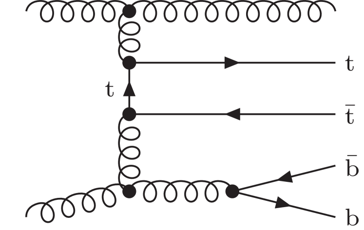
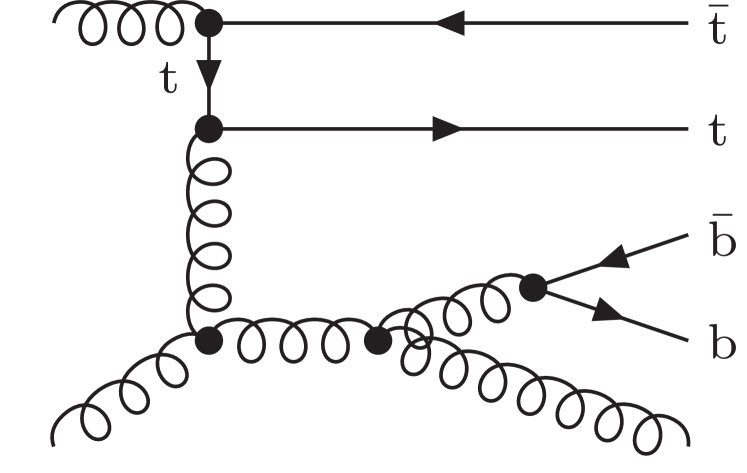
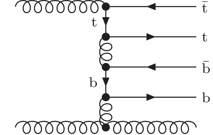
Figure 1: Selected Born diagrams in the $gg\to t\bar{t}b\bar{b}g$ channel.

The independent partonic channels contributing to $pp\to t\bar{t}b\bar{b}j$ at NLO are summarised in Table 1 together with the number of Feynman diagrams and crossing/flavour symmetries. At LO, $t\bar{t}b\bar{b}j$ production involves the two crossing-independent channels $gg\to t\bar{t}b\bar{b}g$ and $q\bar{q}\to t\bar{t}b\bar{b}g$ with $q=d,u,s,c$, where the latter gives rise to six quark–anti-quark and gluon–(anti)quark channels via permutations of $q,\bar{q},g$.

Fig. 1 illustrates sample diagrams for the gluon–gluon channel, which is by far the dominant channel, with a contribution of about $77\%$ ($qg$: $21\%$, $q\bar{q}$: $2\%$). The dominant $gg\to t\bar{t}b\bar{b}g$ topologies are those where the $b\bar{b}$ pair is emitted from a $g\to b\bar{b}$ splitting and the final-state gluon results from an initial-state $g\to gg$ splitting, while the $t\bar{t}$ pair is produced in a $t$-channel configuration. However, the impact of other topologies becomes quite prominent in certain phase-space regions, like e.g. at high invariant mass or $\Delta R$ separation of the $b\bar{b}$ system. See also Fig. 3 for the dominant $gg\to t\bar{t}b\bar{b}$ topologies.

At NLO in QCD, as usually the process receives contributions both from virtual and real corrections, which are separately divergent. To mediate these divergences between the different phase spaces, we rely on the dipole-subtraction formalism Catani:1996vz in its extension to massive QCD partons Catani:2002hc .

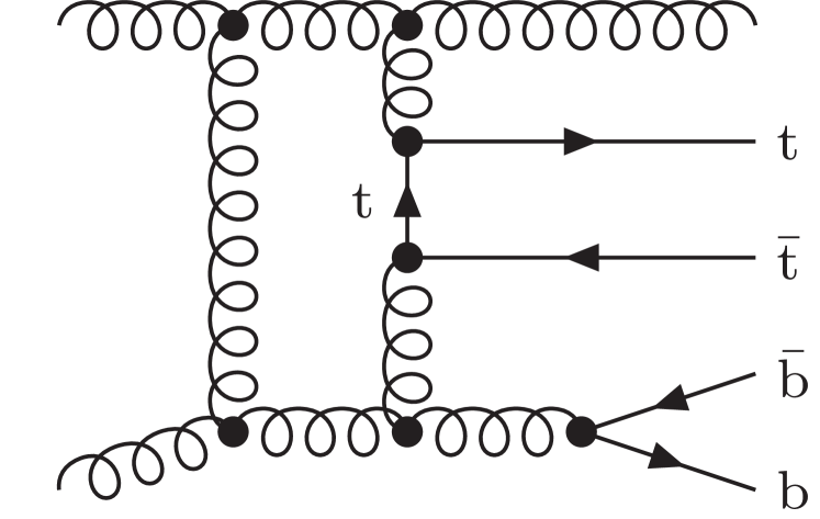
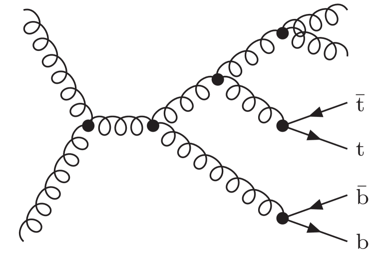
Figure 2: Selected $gg\to t\bar{t}b\bar{b}g$ one-loop diagrams (first row) and $gg\to t\bar{t}b\bar{b}gg$ real-emission diagrams (second row).

The virtual corrections are constituted from both diagrams with a closed quark loop and diagrams that are generated from the LO ones by exchanging a virtual gluon between any of the external or internal legs. Since all involved partons interact under QCD, the number of loop diagrams is more than a factor of 50 larger than the number of Born diagrams in the respective channels (see Table 1). While the quark-loop diagrams contain up to pentagon functions, the gluon-exchange diagrams require up to heptagon functions. Some sample diagrams for the latter are shown in Fig. 2 (first row), again for the dominant $gg$ channel only.

The real-correction channels are constructed from the LO ones by either emission of another gluon or by the splitting of a gluon into a light $q\bar{q}$ pair. Including crossings of light partons between initial and final states, the channels listed in Table 1 result. In Fig. 2 (second row) we depict sample diagrams for the dominant all-gluon channel.

2.2 Tools and validation

The calculations presented in this paper have been performed with the automated frameworks Sherpa+OpenLoops and Munich+OpenLoops. Each of them completes the full chain of operations — from process definition to collider observables — that enter NLO QCD simulations at parton level.

In both frameworks virtual amplitudes are provided by OpenLoops 2 Buccioni:2019sur , the latest version of the OpenLoops matrix-element generator. One of the of main novelties of OpenLoops 2, which is used for the first time in the calculation at hand, is the combination of the original open-loop algorithm Cascioli:2011va with the recently proposed on-the-fly reduction method Buccioni:2017yxi . In this approach, the construction of loop amplitudes and their reduction to scalar integrals are combined in a single numerical recursion, which makes it possible to generate one-loop amplitudes in a way that avoids high tensorial ranks at all stages of the calculations. This results in a significant speed-up for multi-leg processes. Specifically, for the process at hand, the excellent CPU performance of OpenLoops 1 is further improved by a factor of three. For the treatment of numerical instabilities, the on-the-fly reduction algorithm is equipped by an automated stability system that combines analytic expansions together with a novel hybrid-precision system. The latter detects residual instabilities based on the analytic structure of reduction identities and cures them by switching from double (dp) to quadruple (qp) precision. Thanks to the local and highly targeted usage of qp, the typical qp overhead wrt dp evaluation timings is reduced from two orders of magnitude to a few percent.

The only external ingredients required by OpenLoops 2 are the scalar integrals Denner:2010tr , which are provided by the Collier library Denner:2014gla ; Denner:2016kdg by default, or by the OneLOop library vanHameren:2010cp for exceptional qp evaluations. All amplitudes have been thoroughly validated against OpenLoops 1 Cascioli:2011va , where the reduction is carried out based on the Denner–Dittmaier techniques Denner:2002ii ; Denner:2005nn available in Collier or, alternatively, using CutTools Ossola:2007ax , which implements the OPP method Ossola:2006us , together with the OneLOop library vanHameren:2010cp for scalar integrals. Additionally, matrix elements have been cross-checked against the completely independent generator Recola Actis:2016mpe ; Denner:2017wsf .

All remaining tasks, i.e. the bookkeeping of partonic subprocesses, phase-space integration, and the subtraction of QCD bremsstrahlung, are supported by the two independent and fully automated Monte Carlo generators, Munich and Sherpa.

In Sherpa, tree amplitudes are computed using Comix Gleisberg:2008fv , a matrix-element generator based on the colour-dressed Berends-Giele recursive relations Duhr:2006iq , while one-loop amplitudes are provided by OpenLoops. Infrared singularities are cancelled using the dipole subtraction method Catani:1996vz ; Catani:2002hc , as automated in Comix, with the exception of K- and P-operators that are taken from the implementation described in Gleisberg:2007md . Comix is also used for the evaluation of all phase-space integrals. Analyses are performed with the help of Rivet Buckley:2010ar , which involves the FastJet package Cacciari:2005hq ; Cacciari:2011ma to cluster partons into jets.

The parton-level generator Munich has been applied to several multi-leg processes at NLO QCD and EW accuracy, and as a key ingredient of the Matrix framework Grazzini:2017mhc it has been intensively applied to boson and diboson production at NNLO QCD. Munich provides a very efficient multi-channel phase-space integration with several optimizations for higher-order applications. All tree-level and one-loop amplitudes are supplied by OpenLoops through a fully automated interface. The implementation of the massive dipole subtraction formalism used in the present calculation has been extensively tested in the context of off-shell top-pair production in the 4F scheme Cascioli:2013wga , and very recently in the NNLO QCD production of $t\bar{t}$ pairs Catani:2019iny ; Catani:2019hip . The implementation of phase-space cuts at generation and analysis level, as well as the event selection including jet algorithms are realized directly in Munich, without relying on external tools. Also the calculation of arbitrary (multi-)differential observables and the setting of dynamic scales are handled internally. Thereby Munich provides an independent cross-check of basically all remaining steps of the working chain.

Both tools have been validated extensively against each other for a representative selection of the results presented in this paper. All cross sections binned in $b$-jet and light-jet multiplicities (see Tables 3 and 4) have been validated at a precision level of $0.3\%$ throughout for all scale choices. Moreover, most of the differential distributions presented in Section 5 have been cross-checked at the NLO level. For all compared observables we find agreement on the level expected from the statistical uncertainties of the two independent calculations.

3 Technical aspects and setup

In this section we specify the input parameters, PDFs, scale choices and acceptance cuts used in the calculations presented in Sections 4–6.

3.1 Input parameters, PDFs and scale choices

Heavy-quark mass effects are included throughout using

$$m_{t}=172.5\;\text{GeV}\,,\qquad m_{b}=4.75\;\text{GeV}\,.$$ (1)

All other quarks are treated as massless in the perturbative part of the calculations. Since we use massive $b$-quarks, for the PDF evolution and the running of $\alpha_{\mathrm{S}}$ we adopt the 4F scheme. Thus, for consistency, we renormalise $\alpha_{\mathrm{S}}$ in the decoupling scheme, where top- and bottom-quark loops are subtracted at zero momentum transfer. In this way, heavy-quark loop contributions to the evolution of the strong coupling are effectively described at first order in $\alpha_{\mathrm{S}}$ through the virtual corrections.

We present predictions for $pp\to t\bar{t}b\bar{b}j$ at $\sqrt{s}=13$ TeV. At LO and NLO we use throughout the 4F NNPDF parton distributions Ball:2014uwa at NLO, and the corresponding strong coupling. PDF uncertainties are expected to play a rather subleading role, similarly as for $pp\to t\bar{t}b\bar{b}$ Jezo:2018yaf . Thus we will base our predictions on the nominal PDF set, restricting our assessment of theoretical uncertainties to perturbative scale variations.

3.2 Renormalisation and factorisation scales

Since it scales with $\alpha_{\mathrm{S}}^{5}$, the $t\bar{t}b\bar{b}j$ cross section is highly sensitive to the choice of the renormalisation scale $\mu_{\mathrm{R}}$, and this choice plays a critical role for the stability of perturbative predictions. Along the lines of Cascioli:2013era ; deFlorian:2016spz ; Jezo:2018yaf , we adopt a dynamic scale that accounts for the fact that $t\bar{t}b\bar{b}$ production is characterised by two widely separated scales, which are related to the $t\bar{t}$ and $b\bar{b}$ systems. To this end we define

$$\mu^{2}_{b\bar{b}}=E_{\mathrm{T},b}E_{\mathrm{T},\bar{b}},\qquad\mu^{2}_{t\bar{t}}=E_{\mathrm{T},t}E_{\mathrm{T},\bar{t}},\qquad m^{2}_{b\bar{b}}=(p_{b}+p_{\bar{b}})^{2}\,,$$ (2)

where the transverse energies $E_{\mathrm{T},i}=\sqrt{m_{i}^{2}+p^{2}_{\mathrm{T},i}}$ are defined in terms of the rest masses $m_{i}$ and the transverse momenta $p_{\mathrm{T},i}$ of the bare heavy quarks, without applying any jet algorithm at NLO. Also ${m^{2}_{b\bar{b}}}$ is defined in terms of the bare four-momenta of the (anti-)$b$ quarks. As default choice for the renormalisation scale we adopt the geometric average of the various transverse energies and momenta of the $t\bar{t}b\bar{b}j$ system,

$${\mu}_{t\bar{t}b\bar{b}j}\,(\xi_{\mathrm{R}}) = \xi_{\mathrm{R}}\,{\mu}_{t\bar{t}b\bar{b}j}\,=\,\xi_{\mathrm{R}}\Big{(}\mu^{2}_{t\bar{t}}\,\mu^{2}_{b\bar{b}}\,p_{\mathrm{T},j}\Big{)}^{1/5},$$ (3)

where the rescaling factor $\xi_{\mathrm{R}}$ is typically varied in the range $[0.5,2]$. This choice represents the natural generalisation of the widely used scale Cascioli:2013era ; deFlorian:2016spz ; Jezo:2018yaf

$${\mu}_{t\bar{t}b\bar{b}}\,(\xi_{\mathrm{R}}) = \xi_{\mathrm{R}}\,{\mu}_{t\bar{t}b\bar{b}}\,=\,\xi_{\mathrm{R}}\left(\mu_{t\bar{t}}\,\mu_{b\bar{b}}\right)^{1/2}$$ (4)

for $t\bar{t}b\bar{b}$ production. The additional light-jet $p_{\mathrm{T}}$ that enters (3) is defined using an auxiliary $k_{\mathrm{T}}$-jet algorithm with $R=0.4$, which is applied only to massless partons, i.e. excluding top and bottom quarks from the recombination, and is free from any restriction in $p_{\mathrm{T}}$ and rapidity.

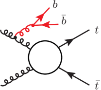
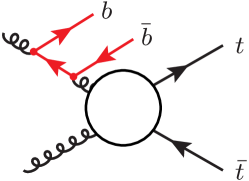
Figure 3: Generic leading-order $gg\to t\bar{t}b\bar{b}$ topologies with final-state (a) and initial-state (b) $g\to b\bar{b}$ splittings. The bulk of the $t\bar{t}b\bar{b}$ cross section is dominated by topologies of type (a) with rather collinear splittings, while initial-state collinear splittings become important in the region of large $\Delta R_{bb}$ Jezo:2018yaf .

In order to assess shape uncertainties, we consider three alternative dynamic scales with different kinematic dependences. The first one is defined as

$${\mu}_{gb\bar{b}}(\xi_{\mathrm{R}})\,=\,\xi_{\mathrm{R}}\,{\mu}_{gb\bar{b}}\,=\,\left(\mu^{2}_{t\bar{t}}\,m_{b\bar{b}}\,E_{\mathrm{T},b\bar{b}}\,p_{\mathrm{T},j}\right)^{1/5},$$ (5)

where the $b\bar{b}$ system enters through its invariant mass and its total transverse energy, $E_{\mathrm{T},b\bar{b}}=\sqrt{m_{b\bar{b}}^{2}+(\vec{p}_{\mathrm{T},b}+\vec{p}_{\mathrm{T},\bar{b}})^{2}}$. This choice is motivated by the fact that $m_{b\bar{b}}$ and $E_{\mathrm{T},b\bar{b}}$ correspond to the virtualities of the QCD branching processes that dominate $t\bar{t}b\bar{b}$ production, namely initial-state $g\to gg$ splittings followed by a final-state $g\to b\bar{b}$ splittings (see Fig. 3).

As further alternatives we consider two other dynamic scales,

$${\mu}_{\mathrm{T},\mathrm{tot}}\,(\xi_{\mathrm{R}}) = \xi_{\mathrm{R}}\,{\mu}_{\mathrm{T},\mathrm{tot}}=\xi_{\mathrm{R}}\frac{H_{\mathrm{T}}}{5},$$ (6)

and

$${\mu}_{\mathrm{T},\mathrm{jets}}\,(\xi_{\mathrm{R}}) = \xi_{\mathrm{R}}\,{\mu}_{\mathrm{T},\mathrm{jets}}\,=\,\xi_{\mathrm{R}}\left(\mu_{t\bar{t}}\,\frac{H_{\mathrm{T},\mathrm{jets}}}{3}\right)^{1/2}\,,$$ (7)

which are defined in terms of the transverse energies of the jets,

$$H_{\mathrm{T},\mathrm{jets}}=\sum_{i=b,\bar{b},g,q,\bar{q}}E_{\mathrm{T},i}\,,$$ (8)

and the total transverse energy,

$$H_{\mathrm{T}}=H_{\mathrm{T},\mathrm{jets}}+\sum_{i=t,\bar{t}}E_{\mathrm{T},i}\,.$$ (9)

Here $E_{\mathrm{T},j}=p_{\mathrm{T},j}$ for massless partons, and the sums run over all final-state QCD partons, always including NLO radiation and excluding only top quarks in the case of $H_{\mathrm{T},\mathrm{jets}}$.

The factorisation scale $\mu_{\mathrm{F}}$ represents the maximum transverse momentum for initial-state radiation that is resummed in the PDFs. Thus it is typically chosen of the order of the halved hard-scattering energy. Following Cascioli:2013era ; Jezo:2018yaf we use

$$\mu_{\mathrm{F}}=\xi_{\mathrm{F}}\,\frac{H_{\mathrm{T}}}{2}\;,$$ (10)

where $\xi_{\mathrm{F}}\in[0.5,2]$.

Our nominal predictions correspond to $\xi_{\mathrm{R}}=\xi_{\mathrm{F}}=1$, and to quantify scale uncertainties we take the envelope of the seven-point variation $(\xi_{\mathrm{R}},\xi_{\mathrm{F}})=(0.5,0.5)$, $(0.5,1)$, $(1,0.5)$, $(1,1)$, $(1,2)$, $(2,1)$, $(2,2)$.

3.3 Jet observables and acceptance cuts

region	ttb	ttbb	ttbj	ttbbj	ttbjj	ttbbjj
$N^{\mathrm{min}}_{b}$	1	2	1	2	1	2
$N^{\mathrm{min}}_{j}$	0	0	1	1	2	2

Table 2: Naming scheme for phase-space regions with different inclusive multiplicities of $b$-jets ($N_{b}\geq N^{\mathrm{min}}_{b}$) and light jets ($N_{j}\geq N^{\mathrm{min}}_{j}$) that pass the acceptance cuts (11).

For the reconstruction of jets we use the anti-$k_{\mathrm{T}}$ Cacciari:2008gp algorithm with $R=0.4$. We select $b$-jets and light jets that fulfil the acceptance cuts

$$p_{\mathrm{T}}>p^{\mathrm{cut}}_{\mathrm{T}} = 50\,\text{GeV},\qquad|\eta|<2.5\,.$$ (11)

We define as $b$-jet a jet that contains at least one $b$-quark, i.e. jets that contain a $b\bar{b}$ pair arising from a collinear $g\to b\bar{b}$ splitting are also tagged as $b$-jets. Top quarks are kept stable throughout. When studying $t\bar{t}b\bar{b}j$ production, we categorise events according to the number $N_{b}$ of $b$-jets and the number $N_{j}$ of light jets that fulfil the acceptance cuts (11). We always consider inclusive phase-space regions with $N_{b}\geq N^{\mathrm{min}}_{b}$ and $N_{j}\geq N^{\mathrm{min}}_{j}$, and we label them as indicated in Table 2. For the analysis of cross sections and distributions, we always require one additional jet, and we consider an inclusive ttbj selection ($N^{\mathrm{min}}_{b}=1$) and a more exclusive ttbbj selection ($N^{\mathrm{min}}_{b}=2$).

4 Integrated cross sections for $\boldsymbol{pp\to t\bar{t}b\bar{b}j}$ at 13 TeV

In this section we present numerical predictions for $pp\to t\bar{t}b\bar{b}j$ at $\sqrt{s}=13$ TeV in the 4F scheme. The results have been obtained with Sherpa+OpenLoops and Munich+OpenLoops, using the setup of Section 3. Top quarks are kept stable throughout, and we study cross sections and distributions in the inclusive ttbj and ttbbj phase-space regions as defined in Table 2, applying the acceptance cuts (11). Perturbative scale uncertainties are assessed by means of seven-point factor-two scale variations and by comparing the various dynamic scales defined in Section 3.2.

4.1 Renormalisation scale dependence

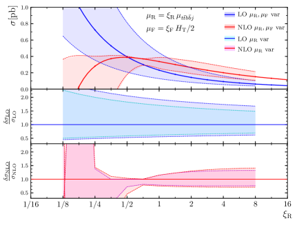
Figure 4: Cross sections at $\sqrt{s}=13\,$TeV in the ttbbj phase space. Predictions at LO (blue) and NLO (red) with scales $\mu_{\mathrm{R}}=\xi_{\mathrm{R}}{\mu}_{t\bar{t}b\bar{b}j}$ and $\mu_{\mathrm{F}}=H_{\mathrm{T}}/2$ are plotted as a function of the renormalisation scale factor $\xi_{\mathrm{R}}$. The main frame presents absolute predictions and corresponding 7-point factor-two variations of $\mu_{\mathrm{R}}$ and $\mu_{\mathrm{F}}$, which are shown as uncertainty bands. The relative impact of such variations at LO and NLO is displayed in the two ratio plots, which show also a second uncertainty band corresponding to pure factor-two variations of $\mu_{\mathrm{R}}$ at fixed $\mu_{\mathrm{F}}=H_{\mathrm{T}}/2$.

A first picture of the perturbative behaviour of the $t\bar{t}b\bar{b}j$ cross section is displayed in Fig. 4, where LO and NLO predictions based on the nominal scale choice (3) are plotted as a function of the renormalisation scale $\mu_{\mathrm{R}}$. For each value of $\mu_{\mathrm{R}}$, the effect of factor-two scale variations is illustrated through two bands, which correspond to the variation of $\mu_{\mathrm{R}}$ alone and the full 7-point variation of $\mu_{\mathrm{R}}$ and $\mu_{\mathrm{F}}$. The results demonstrate that $\mu_{\mathrm{F}}$ variations play only a marginal role, especially at NLO. Thus, in the following we will focus on the $\mu_{\mathrm{R}}$ dependence.

Figure 5: Renormalisation-scale dependence of the LO (dashed) and NLO (dotted) cross sections at $\sqrt{s}=13\,$TeV in the ttbbj phase space. The different curves correspond to the four dynamic scales defined in (3),(5)–(7). More precisely, instead of ${\mu}_{\mathrm{T},\mathrm{tot}}=H_{\mathrm{T}}/5$, the scale $H_{\mathrm{T}}$/4 is shown in this plot. Each scale is varied around its nominal value ($\xi_{\mathrm{R}}=1$) by a factor $\xi_{\mathrm{R}}\in[1/16,16]$, and the factorisation scale is kept fixed at $\mu_{\mathrm{F}}=H_{\mathrm{T}}/2$. Absolute predictions are shown in the main frame, while the ratio plot shows the NLO correction factor $K(\xi_{\mathrm{R}})=\sigma_{\mathrm{NLO}}(\xi_{\mathrm{R}})/\sigma_{\mathrm{LO}}(\xi_{\mathrm{R}})$.

In Fig. 5 we plot the LO and NLO $t\bar{t}b\bar{b}j$ cross section as a function of $\mu_{\mathrm{R}}$ for all four dynamical scales defined in (3),(5)–(7). For each choice the renormalisation scale is varied around its nominal value by a factor $\xi_{\mathrm{R}}\in[1/16,16]$, while the factorisation scale is kept fixed at $\mu_{\mathrm{F}}=H_{\mathrm{T}}/2$. The behaviour of the LO curves in Fig. 5 reflects the $\alpha_{\mathrm{S}}$-dependence of the LO cross section, $\sigma_{\mathrm{LO}}\propto\alpha_{\mathrm{S}}^{5}$, and corresponds essentially to the running of $\alpha_{\mathrm{S}}$ to the fifth power. To discuss the qualitative behaviour of Fig. 5 in more detail, let us consider the effect of $\mu_{\mathrm{R}}\to\xi\mu_{\mathrm{R}}$ rescalings at LO,

$$\alpha_{\mathrm{S}}(\xi\,\mu_{\mathrm{R}}) = \alpha_{\mathrm{S}}(\mu_{\mathrm{R}})\big{[}1+a_{0}(\mu_{\mathrm{R}})\ln\xi\big{]}^{-1}\,.$$ (12)

Here $a_{0}(\mu_{\mathrm{R}})=b_{0}\alpha_{\mathrm{S}}(\mu_{\mathrm{R}})/(2\pi)=\ln^{-1}(\mu_{\mathrm{R}}/\Lambda_{\mathrm{QCD}})$, and for small variations $\delta\xi$,

$$\frac{\delta\alpha_{\mathrm{S}}^{5}}{\alpha_{\mathrm{S}}^{5}}=-5a_{0}(\mu)\,\frac{\delta\xi}{\xi}\,.$$ (13)

This is consistent with the LO curves of Fig. 5, where we observe that around the nominal scales ($\xi=1$), reducing $\mu_{\mathrm{R}}$ by a factor 2 augments the LO cross sections by a factor close to 2 and vice versa, which corresponds to $5a_{0}(\mu)\sim 1$.

At NLO, the one-loop $\alpha_{\mathrm{S}}$-counterterm cancels the $\xi$-dependence at $\mathcal{O}(\alpha_{\mathrm{S}}\ln\xi)$, resulting in a significant reduction of scale variations. In the vicinity of the nominal scales, factor-two variations go down to 10–25%, depending on the type of scale and the direction of the variation. As usually, the various NLO curves feature a stable point, which is located between $\xi_{\mathrm{R}}=1/2$ and $1/3$. In the region below the maximum, the NLO curves start falling quite fast, and between $\xi_{\mathrm{R}}=$1/6 and $1/8$ they lead to negative cross sections. To avoid such a pathologic perturbative behaviour, the normalisation factors in the definition of ${\mu}_{\mathrm{T},\mathrm{tot}}$ and ${\mu}_{\mathrm{T},\mathrm{jets}}$ have been chosen in such a way that factor-two variations of the nominal scales do not enter the region below the NLO maximum. Concerning the NLO correction factors, $K=\sigma_{\mathrm{NLO}}/\sigma_{\mathrm{LO}}$, at $\xi_{\mathrm{R}}\simeq 1$ we find $K\sim 1.5$ while the $K$-factor approaches one in the vicinity of the NLO maxima of the respective curves.

A striking feature of Fig. 5 is that, in spite of the rather different kinematic dependence of the various dynamic scales, the observed LO and NLO scale variations and $K$-factors have a fairly similar shape. In order to gain more insights into the origin of this behaviour, in the following we focus on the $\alpha_{\mathrm{S}}$-dependence of the LO cross section. For the differential and integrated cross sections let us define

$$\mathrm{d}\sigma_{\mathrm{LO}}\big{(}\mu_{\mathrm{dyn}}(\Phi)\big{)}=\alpha_{\mathrm{S}}^{5}\big{(}\mu_{\mathrm{dyn}}(\Phi)\big{)}\,\mathrm{d}\hat{\sigma}_{\mathrm{LO}},\qquad\hat{\sigma}_{\mathrm{LO}}=\int\mathrm{d}\hat{\sigma}_{\mathrm{LO}}\,=\,\int\mathrm{d}\Phi\,\,\frac{\mathrm{d}\hat{\sigma}_{\mathrm{LO}}}{\mathrm{d}\Phi}\,,$$ (14)

where $\mu_{\mathrm{dyn}}(\Phi)$ is a certain dynamic scale, $\Phi$ stands for the fully-differential final-state phase space, and the convolution with PDFs as well as acceptance cuts are implicitly understood. For the integrated cross section with dynamic scale $\mu_{\mathrm{dyn}}$ we can write

$$\sigma_{\mathrm{LO}}(\mu_{\mathrm{dyn}}) = \int{\mathrm{d}\hat{\sigma}_{\mathrm{LO}}}\,\alpha_{\mathrm{S}}^{5}\big{(}\mu_{\mathrm{dyn}}(\Phi)\big{)}\,=\,\alpha_{\mathrm{S}}^{5}\left(\bar{\mu}_{\mathrm{dyn}}\right)\hat{\sigma}_{\mathrm{LO}}\,,$$ (15)

where the result is expressed in terms of the $\alpha_{\mathrm{S}}$-free cross section $\hat{\sigma}_{\mathrm{LO}}$ and the coupling factor $\alpha_{\mathrm{S}}^{5}(\bar{\mu}_{\mathrm{dyn}})$, which corresponds to the average of $\alpha_{\mathrm{S}}^{5}\left(\mu_{\mathrm{dyn}}(\Phi)\right)$. The above identity is nothing but a definition of the “average” scale $\bar{\mu}_{\mathrm{dyn}}$, which depends both on the functional form of $\mu_{\mathrm{dyn}}(\Phi)$ and on the applied phase-space cuts. Let us now consider scale variations,

$$\sigma_{\mathrm{LO}}(\xi\,\mu_{\mathrm{dyn}}) = \int{\mathrm{d}\hat{\sigma}_{\mathrm{LO}}}\,\alpha_{\mathrm{S}}^{5}\big{(}\xi\,\mu_{\mathrm{dyn}}(\Phi)\big{)}\,.$$ (16)

The effect of $\mu_{\mathrm{dyn}}\to\xi\,\mu_{\mathrm{dyn}}$ on $\alpha_{\mathrm{S}}\big{(}\mu_{\mathrm{dyn}}(\Phi)\big{)}$ can be expressed as

$$\alpha_{\mathrm{S}}\big{(}\xi\,\mu_{\mathrm{dyn}}(\Phi)\big{)} = \alpha_{\mathrm{S}}(\xi\,\bar{\mu}_{\mathrm{dyn}})\left[1+a_{0}(\xi\,\bar{\mu}_{\mathrm{dyn}})\ln\left(\frac{\xi\,\mu_{\mathrm{dyn}}(\Phi)}{\xi\,\bar{\mu}_{\mathrm{dyn}}}\right)\right]^{-1}$$ (17)

$$= \alpha_{\mathrm{S}}(\xi\,\bar{\mu}_{\mathrm{dyn}})\sum_{n=0}^{\infty}\left[-a_{0}(\xi\,\bar{\mu}_{\mathrm{dyn}})\ln\left(\frac{\mu_{\mathrm{dyn}}(\Phi)}{\bar{\mu}_{\mathrm{dyn}}}\right)\right]^{n}\,,$$

where the $\alpha_{\mathrm{S}}(\xi\,\bar{\mu}_{\mathrm{dyn}})$ prefactor on the rhs corresponds to a trivial rescaling of $\bar{\mu}_{\mathrm{dyn}}$, while the term between square brackets depends on all moments of the distribution in $\ln\left(\mu_{\mathrm{dyn}}(\Phi)\right)$,

$$\big{\langle}\ln^{n}(\mu_{\mathrm{dyn}})\big{\rangle} = \frac{1}{\hat{\sigma}_{\mathrm{LO}}}\int\mathrm{d}\hat{\sigma}_{\mathrm{LO}}\,\left[\ln\big{(}\mu_{\mathrm{dyn}}(\Phi)\big{)}\right]^{n}\,.$$ (18)

Such moments may influence the scale dependence in a non-trivial way. However, their actual impact on the integrated cross section turns out to be marginal. This is due to the fact that QCD cross sections are typically dominated by phase-space regions with well-defined energy scales in the vicinity of the thresholds for producing massive final states and passing acceptance cuts. As a consequence, the distribution in $\ln\left(\mu_{\mathrm{dyn}}(\Phi)\right)$ is confined in the vicinity of its average value, $\ln(\bar{\mu}_{\mathrm{dyn}})$, and its higher moments are rather strongly suppressed. This implies

$$\big{\langle}\ln^{n}(\mu_{\mathrm{dyn}})\big{\rangle} \simeq \ln^{n}(\bar{\mu}_{\mathrm{dyn}})\,,$$ (19)

for all $n\geq 1$. More precisely, let us assume that

$$X_{n} = a^{n}_{0}(\xi\,\bar{\mu}_{\mathrm{dyn}})\big{\langle}\big{(}\ln(\mu_{\mathrm{dyn}})-\ln(\bar{\mu}_{\mathrm{dyn}})\big{)}^{n}\big{\rangle}\ll 1\,,$$ (20)

for $n\geq 2$. This implies that the expectation value of the rhs of (17) is dominated by the $n=0$ term. Thus, under the above assumptions, the scale dependence of the LO cross sections (16) can be approximated as

$$\sigma_{\mathrm{LO}}(\xi\,\mu_{\mathrm{dyn}}) \simeq \,\alpha_{\mathrm{S}}^{5}\left(\xi\,\bar{\mu}_{\mathrm{dyn}}\right)\hat{\sigma}_{\mathrm{LO}}\,,$$ (21)

i.e. by a naive rescaling of $\alpha_{\mathrm{S}}^{5}\left(\bar{\mu}_{\mathrm{dyn}}\right)$.

We have verified that this property is fulfilled with percent-level accuracy by all LO curves of Fig. 5. This means that, at the level of the integrated cross section, the various scales (3),(5)–(7) are equivalent to each other. More precisely, the scale dependence of $\sigma_{\mathrm{LO}}$ with a given dynamic scale $\mu_{\mathrm{dyn},k}$ can be related to the one of a fixed scale $\mu_{0}$ by means of a constant rescaling

$$\mu_{\mathrm{dyn},k}(\Phi) \to {\tilde{\mu}}_{\mathrm{dyn},k}(\Phi)\,=\,\chi_{k}\,\mu_{\mathrm{dyn},k}(\Phi)\,,\qquad\mbox{with}\quad\chi_{k}=\frac{\mu_{0}}{\bar{\mu}_{\mathrm{dyn},k}}\,,$$ (22)

which results into

$$\sigma_{\mathrm{LO}}(\xi{\tilde{\mu}}_{\mathrm{dyn},k}) \simeq \sigma_{\mathrm{LO}}(\xi\mu_{0})\,.$$ (23)

Therefore, as far as the scale uncertainty of $\sigma_{\mathrm{LO}}$ and its normalisation are concerned, comparing different types of dynamic scales has no significant added value wrt simple $\xi_{\mathrm{R}}$-rescalings. For this reason, we advocate the usage of “aligned” dynamic scales ${\tilde{\mu}}_{\mathrm{dyn},k}$, as defined in (22). In this way, the various dynamic scales have the same average value, and the uncertainties related to this common average value are accounted for by standard $\xi_{\mathrm{R}}$-rescalings, while the comparison of different scale definitions allows one to highlight the genuine kinematic effects that are inherent in their dynamic nature. Comparing aligned dynamic scales yields no significant effect at the level of integrated cross sections, but provides key information on shape uncertainties, since the average scales $\bar{\mu}_{\mathrm{dyn},k}$ are sensitive both to the probed phase-space regions and to the detailed kinematic dependence of $\mu_{\mathrm{dyn},k}(\Phi)$. Vice versa, $\xi$-rescalings can be used to assess uncertainties in the normalisation of $\sigma_{\mathrm{LO}}$, whereas their impact on shapes is typically quite limited.

At LO, the above-mentioned alignment approach misses a crucial ingredient, namely a good criterion for the choice of a reference scale $\mu_{0}$. For $pp\to t\bar{t}b\bar{b}j$, due to the very strong scale dependence induced by $\alpha_{\mathrm{S}}^{5}$, the choice of a well-behaved central scale is of crucial importance. At the same time, the presence of multiple scales, distributed from $m_{b}$ to $m_{t\bar{t}}$ and beyond, renders this choice non-trivial. At NLO, a natural way of addressing the scale-choice problem is to exploit the presence of a characteristic scale given by the maximum of the NLO scale-dependence curves, $\mu_{\mathrm{max}}$. The maximum itself is not necessarily an optimal scale choice, since its position is not guaranteed to be stable wrt higher-order corrections. Moreover, the flatness of the scale dependence around $\mu_{\mathrm{R}}=\mu_{\mathrm{max}}$ tends to underestimate scale uncertainties. A more reasonable and conservative option, that will be adopted in this paper, is to set the central scale at $\mu_{\mathrm{R}}\simeq 2\mu_{\mathrm{max}}$. In this way, the range of factor-two scale variations extends over $[\mu_{\mathrm{max}},4\,\mu_{\mathrm{max}}]$, covering the maximum itself as well as a relatively broad region where $\sigma_{\mathrm{NLO}}$ is monotonically decreasing.

Figure 6: Renormalisation-scale dependence of the $t\bar{t}b\bar{b}j$ cross section at $\sqrt{s}=13\,$TeV. Same predictions and variations as in Fig. 5, but with the aligned central scales defined in (24).

As observed in Fig. 5, the position of $\mu_{\mathrm{max}}$ depends on the choice of the dynamic scale. However, for reasons similar to those discussed above at LO, also NLO scale variations and the position of their maxima can be aligned via rescalings. This is not entirely obvious and does not work as precisely as in the LO case. The main reason is that NLO cross sections consist of two kind of contributions: Born and virtual parts, which are distributed in a similar way as $\mathrm{d}\hat{\sigma}_{\mathrm{LO}}$, and real-emission parts that can be distributed in a significantly different way. Moreover, dynamic scales can feature a different sensitivity to the kinematics of hard jet radiation, leading to genuinely new scale-dependence effects at NLO. For these reasons, the LO scale-dependence model (14)–(23) should be refined by splitting $\sigma_{\mathrm{NLO}}$ into two parts with independent average scales. Nevertheless, for the process at hand and the scale choices (3),(5)–(7), it turns out that a single overall rescaling can already yield a good level of NLO alignment.

This is illustrated in Fig. 6, where the dynamic scales (5)–(7) have been rescaled in such a way that the positions of the NLO maxima match the maximum of $\sigma_{\mathrm{NLO}}({\mu}_{t\bar{t}b\bar{b}j})$, which is located at $0.45\,{\mu}_{t\bar{t}b\bar{b}j}$, i.e. ${\mu}_{t\bar{t}b\bar{b}j}$ is rather close to $2\mu_{\mathrm{max}}$. This alignment is achieved by setting

$${\tilde{\mu}}_{t\bar{t}b\bar{b}j} = {\mu}_{t\bar{t}b\bar{b}j}\,,$$

$${\tilde{\mu}}_{gb\bar{b}} = 0.806\,{\mu}_{gb\bar{b}}\,,$$

$${\tilde{\mu}}_{\mathrm{T},\mathrm{jets}} = 1.14\,{\mu}_{\mathrm{T},\mathrm{jets}}\,,$$

$${\tilde{\mu}}_{\mathrm{T},\mathrm{tot}} = 0.853\,\frac{H_{\mathrm{T}}}{4}\,=\,1.066\,{\mu}_{\mathrm{T},\mathrm{tot}}\,,$$ (24)

The fact that the aligned scales are rather close to the original choices (3),(5)–(7) is due to the fact that the latter had already been placed on purpose about two times above the maximum, but without tuning their position in a precise way. As a result of the alignment of the NLO maxima, in Fig. 6 we observe that the predictions based on the two scales that depend on the jet transverse energy, i.e. ${\mu}_{\mathrm{T},\mathrm{tot}}$ and ${\mu}_{\mathrm{T},\mathrm{jets}}$, overlap almost perfectly, both at LO and NLO. A similarly good alignment is observed also between the other two scales, ${\mu}_{t\bar{t}b\bar{b}j}$ and ${\mu}_{gb\bar{b}}$, which do not depend on $H_{\mathrm{T}}$. Vice versa, the scales that do and do not depend on $H_{\mathrm{T}}$ feature a non-negligible difference. In particular, the values of $\sigma_{\mathrm{NLO}}$ at the maxima differ by about 10%. Such differences are most likely due to the fact that the dependence on $H_{\mathrm{T}}$, which is sensitive to NLO radiation, leads to a significant difference between the average scales in Born-like and real-emission contributions at NLO. Nevertheless, we observe that for all curves the position of the maximum coincides quite precisely with the intersection of the NLO and LO curves, which corresponds to $K=1$. Moreover, the four $K$-factors coincide almost exactly in the whole $\xi_{\mathrm{R}}$ range.

In summary, applying a rescaling that aligns dynamic scales based on the positions of the NLO maxima makes it possible to remove trivial differences related to the scale normalisation and to highlight genuine differences related to their kinematic dependence. Since such alignment is in part already realised in the original scale choices (3),(5)–(7), in the following we will refrain from applying the small extra rescaling (24).

$\mu_{\mathrm{R}}$	$N^{\mathrm{min}}_{b}$	$N^{\mathrm{min}}_{j}$	$\sigma_{\mathrm{LO}}$[pb]	$K$	$\sigma_{\mathrm{NLO}}$[pb]	$\dfrac{\sigma_{\mathrm{LO}}^{(N^{\mathrm{min}}_{j})}}{\sigma_{\mathrm{LO}}^{(N^{\mathrm{min}}_{j}-1)}}$	$\dfrac{\sigma_{\mathrm{NLO}}^{(N^{\mathrm{min}}_{j})}}{\sigma_{\mathrm{NLO}}^{(N^{\mathrm{min}}_{j}-1)}}$
ttb	1	0	$3.951^{+73\%}_{-39\%}$	1.92	$7.58^{+32\%}_{-27\%}$
ttbb	2	0	$0.3738^{+70\%}_{-38\%}$	1.80	$0.674^{+27\%}_{-25\%}$
ttbj	1	1	$2.166^{+97\%}_{-45\%}$	1.56	$3.38^{+21\%}_{-27\%}$	0.55	0.45
ttbbj	2	1	$0.2316^{+92\%}_{-45\%}$	1.45	$0.337^{+15\%}_{-25\%}$	0.62	0.50
ttbjj	1	2	$0.7812^{+119\%}_{-51\%}$			0.36
ttbbjj	2	2	$0.08711^{+113\%}_{-50\%}$			0.38

Table 3: Cross sections at LO and NLO for $pp\to t\bar{t}b\bar{b}+$jets at $\sqrt{s}=13\,$TeV. Results are shown for integrated regions with different numbers of $b$-jets, $N^{\mathrm{min}}_{b}=1,2$, and extra light jets, $N^{\mathrm{min}}_{j}=0,1,2$. The acceptance cuts (11) are applied. Predictions for $N^{\mathrm{min}}_{j}=0$ are based on a $t\bar{t}b\bar{b}$ calculation with $\mu_{\mathrm{R}}={\mu}_{t\bar{t}b\bar{b}}$ and $\mu_{\mathrm{F}}=H_{\mathrm{T}}/2$, while $N^{\mathrm{min}}_{j}=1,2$ cross sections correspond to a $t\bar{t}b\bar{b}j$ NLO calculation with $\mu_{\mathrm{R}}={\mu}_{t\bar{t}b\bar{b}j}$ and $\mu_{\mathrm{F}}=H_{\mathrm{T}}/2$. Seven-point scale variations are quoted in percent. In the last two columns, for $N^{\mathrm{min}}_{j}=1,2$ we report the ratios of LO (or NLO) cross sections with $N^{\mathrm{min}}_{j}$ and $(N^{\mathrm{min}}_{j}-1)$. The numerators and denominators of such ratios are computed at the same order.

4.2 Fiducial cross sections

In this section we present detailed numerical results for integrated cross sections and scale uncertainties.

To highlight the quantitative importance of light-jet radiation emitted by the $t\bar{t}b\bar{b}$ system, in Table 3 we present $t\bar{t}b\bar{b}+$jets cross sections with variable $b$-jet and light-jet multiplicities. Comparing the cross sections in the ttbbj and ttbb phase spaces, both available at NLO, we observe that the production rate for an extra light jet is around 50%, i.e. every second $t\bar{t}b\bar{b}$ event involves a hard light jet with $p_{\mathrm{T}}>50$ GeV. The ratio of the cross sections in the ttbbjj and ttbbj regions is around 40%, i.e. the emission of a second extra jet seems to be less abundant. However, one should keep in mind that this ratio is only LO accurate. The light-jet emission rates observed in the phase space with $N^{\mathrm{min}}_{b}=1$ are comparably large to the $N^{\mathrm{min}}_{b}=2$ case. For fixed $N^{\mathrm{min}}_{j}$, cross sections with two $b$-jets are about a factor ten smaller wrt the corresponding cross sections with one $b$-jet. In general, LO scale uncertainties are very large, and grow by roughly 20% at each extra emission. Instead, scale uncertainties at NLO are drastically reduced, and in $t\bar{t}b\bar{b}j$ production they are less pronounced than in $t\bar{t}b\bar{b}$ production.

$\mu_{\mathrm{R}}$	$N^{\mathrm{min}}_{b}$	$\sigma_{\mathrm{LO}}$[pb]	$K$	$\sigma_{\mathrm{NLO}}$[pb]	$\dfrac{\sigma_{\mathrm{LO}}}{\sigma_{\mathrm{LO,def}}}-1$	$\dfrac{\sigma_{\mathrm{NLO}}}{\sigma_{\mathrm{NLO,def}}}-1$
${\mu}_{t\bar{t}b\bar{b}j}$	1	$2.166^{+97\%}_{-45\%}$	1.56	$3.38^{+21\%}_{-27\%}$	$0\%^{+97\%}_{-45\%}$	$0\%^{+21\%}_{-27\%}$
	2	$0.2316^{+92\%}_{-45\%}$	1.45	$0.337^{+15\%}_{-25\%}$	$0\%^{+92\%}_{-45\%}$	$0\%^{+15\%}_{-25\%}$
${\mu}_{gb\bar{b}}$	1	$1.943^{+93\%}_{-45\%}$	1.62	$3.15^{+23\%}_{-28\%}$	$-10\%^{+74\%}_{-51\%}$	$-7\%^{+14\%}_{-33\%}$
	2	$0.2041^{+89\%}_{-44\%}$	1.56	$0.318^{+19\%}_{-26\%}$	$-11\%^{+67\%}_{-51\%}$	$-6\%^{+12\%}_{-30\%}$
${\mu}_{\mathrm{T},\mathrm{jets}}$	1	$1.772^{+91\%}_{-44\%}$	1.51	$2.68^{+15\%}_{-25\%}$	$-18\%^{+56\%}_{-54\%}$	$-21\%^{-9\%}_{-41\%}$
	2	$0.2100^{+90\%}_{-44\%}$	1.37	$0.287^{+7\%}_{-22\%}$	$-9\%^{+72\%}_{-49\%}$	$-15\%^{-8\%}_{-34\%}$
${\mu}_{\mathrm{T},\mathrm{tot}}$	1	$1.697^{+90\%}_{-44\%}$	1.60	$2.71^{+19\%}_{-26\%}$	$-22\%^{+49\%}_{-56\%}$	$-20\%^{-4\%}_{-41\%}$
	2	$0.2064^{+89\%}_{-44\%}$	1.41	$0.291^{+10\%}_{-23\%}$	$-11\%^{+69\%}_{-50\%}$	$-13\%^{-5\%}_{-34\%}$

Table 4: Cross sections at LO and NLO for $pp\to t\bar{t}b\bar{b}j$ at $\sqrt{s}=13\,$TeV. Results are shown for the fiducial regions with $N^{\mathrm{min}}_{j}=1$ and $N^{\mathrm{min}}_{b}=1$ (ttbj) or $N^{\mathrm{min}}_{b}=2$ (ttbbj). The acceptance cuts (11) are applied. Four different choices of $\mu_{\mathrm{R}}$ as defined in (3),(5)–(7) are compared, while the factorisation scale (10) is used throughout. Columns 3–5 show absolute predictions at LO and NLO, as well as the usual correction factor $K=\sigma_{\mathrm{NLO}}/\sigma_{\mathrm{LO}}$. Uncertainties given in percent correspond to seven-point factor-two variations of $\mu_{\mathrm{R}}$ and $\mu_{\mathrm{F}}$. Columns 6 and 7 show the relative differences between LO and NLO cross sections, respectively, based on the default $\mu_{\mathrm{R}}={\mu}_{t\bar{t}b\bar{b}j}$ and the other dynamical scales. As central values we report ratios obtained with the nominal values of the various scales, while lower (upper) values correspond to the minimum (maximum) of $\sigma_{\mathrm{(N)LO}}(\xi_{\mathrm{R}},\xi_{\mathrm{F}})/\sigma_{\mathrm{(N)LO,def}}-1$, where seven-point variations are restricted to the numerator. The reported cross sections have been computed with Monte Carlo statistical uncertainties at the level of three permille at NLO and below one permille at LO.

In the following we focus on LO and NLO predictions for $t\bar{t}b\bar{b}+$jet production in the ttbj and ttbbj phase-space regions. In Table 4 we compare cross sections and scale variations based on the four dynamic scale choices (3),(5)–(7). For what concerns nominal predictions (without scale variations), the default scale $\mu_{\mathrm{R}}={\mu}_{t\bar{t}b\bar{b}j}$ yields the largest cross sections. At LO, the other predictions are between 10% and 20% lower. The ttbbj ​(ttbj) cross sections based on the $H_{\mathrm{T}}$-dependent scales remain 15% (20%) lower also at NLO. In contrast, the two $H_{\mathrm{T}}$-independent scales agree at the level of 5% at NLO. Comparing the cross sections with one and two $b$-jets, using $H_{\mathrm{T}}$-independent scales we observe a ratio very close to $1/10$, while the other scale choices yield a ratio of $1/9.3$.

Seven-point scale variations at LO are between around $-45\%$ and $+90\%$ for all scale choices, both in the ttbj and ttbbj regions. At NLO they are reduced around 20%, with significant differences depending on the scale choice and the number of $b$-jets. In the ttbbj ​(ttbj) phase space, the half-width of the scale-variation band is around 20% (25%) for the $H_{\mathrm{T}}$-independent scales and about 5% smaller for the $H_{\mathrm{T}}$-dependent ones.

In the last two columns of Table 4, we compare LO and NLO cross sections and seven-point variations of the various dynamic scales, normalising the results to nominal predictions with the default scale choice. The scale-variations bands obtained with the $H_{\mathrm{T}}$-dependent scales are significantly lower than the other bands. At NLO, the variation of the default scale covers the absolute NLO maximum observed in Fig. 5, while the upper variations of the $H_{\mathrm{T}}$-dependent scales are $20$–$30$% lower. Vice versa, the lower variation of the default scale is $10$–$15$% above the corresponding variation of the $H_{\mathrm{T}}$-dependent scales. In the ttbbj ​(ttbj) phase spaces, the variations of the default scale change the nominal cross section by $[-25\,(27)\%,+15\,(21)\%]$, while the envelope of the four variation bands corresponds to $[-34\,(41)\%,+15\,(21)\%]$, which amounts to an increase of the half-band width from 20 (24)% to 25 (31)%, i.e. by 5 (7)%. Vice versa, using the ${\mu}_{\mathrm{T},\mathrm{tot}}$ result as a reference gives a ${\mu}_{\mathrm{T},\mathrm{tot}}$ variation band of $[-23\,(26)\%,+10\,(19)\%]$ and an envelope band of $[-23\,(26)\%,+32\,(51)\%]$, which corresponds to an increase of the half-band width from 17 (23)% to 28 (38%)%, i.e. by 11 (15)%. We also note that the variation bands of the $H_{\mathrm{T}}$-independent scales cover the nominal predictions of the $H_{\mathrm{T}}$-dependent scales, but not vice versa. Based on this observations, we conclude that the somewhat larger seven-point variation of the $H_{\mathrm{T}}$-independent scales should be regarded as a more realistic estimate of scale uncertainties.

$\mu_{\mathrm{R}}$	$N^{\mathrm{min}}_{b}$	$\sigma_{\mathrm{LO}}$[pb]	$K$	$\sigma_{\mathrm{NLO}}$[pb]	$\dfrac{\sigma_{\mathrm{LO}}}{\sigma_{\mathrm{LO,def}}}-1$	$\dfrac{\sigma_{\mathrm{NLO}}}{\sigma_{\mathrm{NLO,def}}}-1$
${\tilde{\mu}}_{t\bar{t}b\bar{b}j}$	1	$2.166^{+97\%}_{-45\%}$	1.56	$3.38^{+21\%}_{-27\%}$	$0\%^{+97\%}_{-45\%}$	$0\%^{+21\%}_{-27\%}$
	2	$0.2316^{+92\%}_{-45\%}$	1.45	$0.337^{+15\%}_{-25\%}$	$0\%^{+92\%}_{-45\%}$	$0\%^{+15\%}_{-25\%}$
${\tilde{\mu}}_{gb\bar{b}}$	1	$2.291^{+97\%}_{-46\%}$	1.48	$3.40^{+16\%}_{-26\%}$	$+6\%^{+109\%}_{-43\%}$	$+0.4\%^{+17\%}_{-26\%}$
	2	$0.2388^{+93\%}_{-45\%}$	1.42	$0.338^{+13\%}_{-24\%}$	$+3\%^{+99\%}_{-43\%}$	$+0.3\%^{+13\%}_{-24\%}$
${\tilde{\mu}}_{\mathrm{T},\mathrm{jets}}$	1	$1.606^{+89\%}_{-44\%}$	1.60	$2.57^{+19\%}_{-26\%}$	$-26\%^{+40\%}_{-58\%}$	$-24\%^{-9\%}_{-43\%}$
	2	$0.1909^{+88\%}_{-44\%}$	1.45	$0.277^{+12\%}_{-24\%}$	$-18\%^{+54\%}_{-53\%}$	$-18\%^{-8\%}_{-37\%}$
${\tilde{\mu}}_{\mathrm{T},\mathrm{tot}}$	1	$1.621^{+89\%}_{-44\%}$	1.64	$2.65^{+21\%}_{-27\%}$	$-25\%^{+41\%}_{-58\%}$	$-21\%^{-5\%}_{-43\%}$
	2	$0.1973^{+88\%}_{-44\%}$	1.44	$0.285^{+12\%}_{-24\%}$	$-15\%^{+60\%}_{-52\%}$	$-15\%^{-5\%}_{-36\%}$

Table 5: Cross sections at LO and NLO for $pp\to t\bar{t}b\bar{b}j$ at $\sqrt{s}=13\,$TeV in the ttbj ($N^{\mathrm{min}}_{b}=1$) and ttbbj ($N^{\mathrm{min}}_{b}=2$) phase spaces. Similar predictions and variations as in Table 4 for the case of the aligned central scales defined in (24).

In Table 5 we present similar results based on the aligned scales (24), which correspond to Fig. 6. The main effect of the alignment is that the LO and NLO cross sections based on the two $H_{\mathrm{T}}$-independent scales become much closer to each other, while predictions based on the $H_{\mathrm{T}}$-dependent scales change in a less significant way. This is mainly due to the fact the original scales ${\mu}_{\mathrm{T},\mathrm{jets}}$ and ${\mu}_{\mathrm{T},\mathrm{tot}}$ are already very close to the corresponding aligned scales in (24). In any case, predictions based on the aligned scales are independent of the initial normalisation of the various scales.

After alignment, we still see significant differences between the predictions with $H_{\mathrm{T}}$-dependent and $H_{\mathrm{T}}$-independent scales. More precisely, due to the fact that the alignment is based on the NLO maximum of the ttbbj cross sections, the spread between $K$-factors in the ttbbj phase space goes down from $0.11$ to $0.03$. Vice versa, the $K$-factor difference in the ttbj phase space increases from $0.11$ to $0.16$. The alignment leads also to a slight reduction of NLO scale uncertainties, and the nominal predictions based on $H_{\mathrm{T}}$-independent scales remain above the NLO bands of $H_{\mathrm{T}}$-dependent scales. Such differences between aligned NLO predictions in different phase-space regions should be regarded as genuine effects of the kinematic dependence of dynamic scales. Thus they play a largely complementary role wrt factor-two scale variations.

4.3 Sudakov effects

Figure 7: Distribution in the $p_{\mathrm{T}}$ of the leading light jet in the soft region for $pp\to t\bar{t}b\bar{b}j$ in the ttbbj phase space. In the left (right) plot $b$-jets are subject to the usual cuts with standard (reduced) $p_{\mathrm{T},b}$ threshold of $50$ GeV (25 GeV). Cuts on the jet-$p_{\mathrm{T}}$ have been lowered to 5 GeV, and all jets are subject to a pseudo-rapidity cut $|\eta|<2.5$. The upper frames show LO (dashed) and NLO (solid) absolute predictions with the default scale choice, $\mu_{\mathrm{R}}={\mu}_{t\bar{t}b\bar{b}j}$ and $\mu_{\mathrm{F}}=H_{\mathrm{T}}/2$. The bands correspond to seven-point scale variations. The ratio plots display relative differences wrt to the nominal NLO predictions.

In this section we address the question of the safeness of the chosen transverse-momentum cut of 50 GeV with respect to higher-order Sudakov logarithms. To investigate such Sudakov effects, which appear in the region where the $p_{\mathrm{T}}$ of the light jet, $p_{\mathrm{T},j}$, becomes small, we relax the cut on $p_{\mathrm{T},j}$ and, in Fig. 7, we study the perturbative behaviour of the $\mathrm{d}\sigma/\mathrm{d}p_{\mathrm{T},j}$ distribution. In the left plot, this is done by keeping the usual $b$-jet cuts at $p^{\mathrm{cut}}_{\mathrm{T}}=50\,$GeV, while in the right plot this threshold is lowered to $p^{\mathrm{cut}}_{\mathrm{T}}=25\,$GeV.

As is well known, the $\mathrm{d}\sigma/\mathrm{d}p_{\mathrm{T},j}$ distribution is logarithmically divergent at LO, while summing such logarithms to all orders in $\alpha_{\mathrm{S}}$ would cancel the divergence and lead to $\mathrm{d}\sigma/\mathrm{d}p_{\mathrm{T}}\to 0$ at small $p_{\mathrm{T}}$. In the fixed-order NLO calculation at hand, this behaviour manifests itself through an increasingly strong shape difference between the LO and NLO distributions at small $p_{\mathrm{T}}$. For $p^{\mathrm{cut}}_{\mathrm{T}}=50\,$GeV, we find that at $p_{\mathrm{T}}\simeq 20\,$GeV the NLO curve develops a Sudakov peak, below which NLO corrections start overcompensating the logarithmic growth of the LO distribution. In correspondence with the Sudakov peak, the NLO cross section is already less than half of the LO one, and below 15 GeV it rapidly falls into the unphysical regime of negative cross sections. This pathologic behaviour of the fixed-order NLO prediction is also reflected by the rapid inflation of NLO scale uncertainties below 40 GeV, while our choice of setting the light-jet $p_{\mathrm{T}}$ cuts at 50 GeV guarantees good stability both for the NLO predictions and their uncertainties.

$p^{\mathrm{cut}}_{\mathrm{T}}$[GeV]		50			25
$p_{\mathrm{T},j}$[GeV]	25	50	100	25	50	100
$\dfrac{\mathrm{d}\sigma_{\mathrm{LO}}/\mathrm{d}p_{\mathrm{T},j}}{\mathrm{d}\sigma_{\mathrm{NLO}}/\mathrm{d}p_{\mathrm{T},j}}$	1.45	0.881	0.699	1.09	0.754	0.639

Table 6: Comparison of the LO and NLO distributions in the leading-jet $p_{\mathrm{T}}$ for $p^{\mathrm{cut}}_{\mathrm{T}}=50$ GeV and $25$ GeV. The results correspond to the ttbbj phase space with the cut $p_{\mathrm{T}}>p^{\mathrm{cut}}_{\mathrm{T}}$ restricted to $b$-jets. The reported values at $p_{\mathrm{T},j}/\mathrm{GeV}=25,50,100$ correspond to the bins $\left[22.4,26.0\right]$, $\left[47.3,55.0\right]$ and $\left[86.0,100\right]$.

As can be seen in the right plot of Fig. 7, reducing the $b$-jet threshold to 25 GeV tends to lower the position of the Sudakov peak by 5 GeV or so. In this case, NLO predictions feature a good perturbative convergence down to 30–35  GeV. The effect of NLO corrections on the jet-$p_{\mathrm{T}}$ distribution for selected values of $p_{\mathrm{T}}$ is reported in Table 6.

5 Differential observables

In this section we study differential observables for $pp\to t\bar{t}b\bar{b}j$ at 13 TeV restricting ourselves to the ttbbj phase space. The main focus of our analysis is on the shapes of distributions and related uncertainties.

5.1 Distributions and shape uncertainties in the ttbbj phase space

In Figures 8–16 we analyse a series of differential distributions showing, for each observable, absolute and normalised distributions as well as six different ratio plots, which quantify the relative effects of seven-point variations and differences between the various dynamic scales. We restrict ourselves to the three dynamic scales (3),(5)–(6), since including or not the scale (7) does not change the overall picture of shape uncertainties. The format of the plots is described in the following and in the caption of Fig. 8, and it is the same for all figures in this section.

The left plot of each Figure contains:

• An upper frame with LO and NLO distributions based on the default scale choice $(\mu_{\mathrm{R}},\mu_{\mathrm{F}})=({\mu}_{t\bar{t}b\bar{b}j},H_{\mathrm{T}}/2)$, as well as the corresponding seven-point variation bands.

• A first ratio plot corresponding to the inverse $K$-factor,

  $$K^{-1}_{\mathrm{(N)LO}}(\xi_{\mathrm{R}},\xi_{\mathrm{F}}) = \frac{\sigma_{\mathrm{(N)LO}}(\xi_{\mathrm{R}}\,{\mu}_{t\bar{t}b\bar{b}j},\xi_{\mathrm{F}}\,\mu_{\mathrm{F}})}{\sigma_{\mathrm{NLO}}({\mu}_{t\bar{t}b\bar{b}j},\mu_{\mathrm{F}})}\,,$$ (25)

  where scale variations are applied only in the numerator.

• A second ratio plot that features the LO and NLO ratios,

  $$R_{\mathrm{(N)LO}}(\mu_{\mathrm{R}}) = \frac{\sigma_{\mathrm{(N)LO}}(\xi_{\mathrm{R}}\,\mu_{\mathrm{R}},\xi_{\mathrm{F}}\,\mu_{\mathrm{F}})}{\sigma_{\mathrm{(N)LO}}(\xi_{\mathrm{R}}\,{\mu}_{t\bar{t}b\bar{b}j},\xi_{\mathrm{F}}\,\mu_{\mathrm{F}})}\,.$$ (26)

  This ratio encodes differences between the dynamic scale $\mu_{\mathrm{R}}={\mu}_{gb\bar{b}}$, defined in (5), and the default scale. Seven-point scale variations are applied in a correlated way to the numerator and the denominator. In this way, the main effect of factor-two variations, which amounts to a nearly constant normalisation shift, cancels out. As a result, the ratio (26) is mostly sensitive to effects that arise from the different kinematic dependence of the considered scales, and cannot be accounted for by factor-two variations of a single scale.

• A third ratio plot that shows the ratio (26) for $\mu_{\mathrm{R}}={\mu}_{\mathrm{T},\mathrm{tot}}$.

The right plot of each figure shows the following normalised distributions and ratios thereof.

• The upper frame displays the LO and NLO normalised distributions,

  $$\mathrm{d}\hat{\sigma}_{\mathrm{(N)LO}}(\xi_{\mathrm{R}}\,\mu_{\mathrm{R}},\xi_{\mathrm{F}}\,\mu_{\mathrm{F}}) = \frac{\mathrm{d}\sigma_{\mathrm{(N)LO}}(\xi_{\mathrm{R}}\,\mu_{\mathrm{R}},\xi_{\mathrm{F}}\,\mu_{\mathrm{F}})}{\sigma_{\mathrm{(N)LO}}(\xi_{\mathrm{R}}\,\mu_{\mathrm{R}},\xi_{\mathrm{R}}\,\mu_{\mathrm{F}})}\,,$$ (27)

  for the default scale $\mu_{\mathrm{R}}={\mu}_{t\bar{t}b\bar{b}j}$. The denominator corresponds to the integrated cross section in the ttbbj phase space, and seven-point variations in the numerator and denominator are correlated. In this way, distributions are always normalised to one, i.e. normalisation effects cancel out, and only shape corrections and uncertainties remain visible.

• The first ratio plot shows the ratio of normalised distributions,

  $$\hat{R}_{\mathrm{(N)LO}}({\mu}_{t\bar{t}b\bar{b}j}) = \frac{\mathrm{d}\hat{\sigma}_{\mathrm{(N)LO}}(\xi_{\mathrm{R}}\,{\mu}_{t\bar{t}b\bar{b}j},\xi_{\mathrm{F}}\,\mu_{\mathrm{F}})}{\mathrm{d}\hat{\sigma}_{\mathrm{NLO}}({\mu}_{t\bar{t}b\bar{b}j},\mu_{\mathrm{F}})}\,,$$ (28)

  based on the default scale. Here seven-point variations are applied only to the numerator, but their normalisation effect cancels out as in (27). Thus the ratio (28) highlights the relative effect of NLO corrections and seven-point variations on the shape of distributions.

• The second ratio plot shows the ratios of normalised distributions at LO,

  $$\overline{R}_{\mathrm{LO}}(\mu_{\mathrm{R}}) = \frac{\mathrm{d}\hat{\sigma}_{\mathrm{LO}}(\xi_{\mathrm{R}}\,\mu_{\mathrm{R}},\xi_{\mathrm{F}}\,\mu_{\mathrm{F}})}{\mathrm{d}\hat{\sigma}_{\mathrm{LO}}({\mu}_{t\bar{t}b\bar{b}j},\mu_{\mathrm{F}})}\,,$$ (29)

  for the three dynamic scales $\mu_{\mathrm{R}}={\mu}_{t\bar{t}b\bar{b}j}$, ${\mu}_{gb\bar{b}}$, ${\mu}_{\mathrm{T},\mathrm{tot}}$. This ratio highlights shape differences between those scales (with seven-point variations) and the nominal default scale.

• The third ratio plot shows the same ratios as defined in (29), but at NLO,

  $$\overline{R}_{\mathrm{NLO}}(\mu_{\mathrm{R}}) = \frac{\mathrm{d}\hat{\sigma}_{\mathrm{NLO}}(\xi_{\mathrm{R}}\,\mu_{\mathrm{R}},\xi_{\mathrm{F}}\,\mu_{\mathrm{F}})}{\mathrm{d}\hat{\sigma}_{\mathrm{NLO}}({\mu}_{t\bar{t}b\bar{b}j},\mu_{\mathrm{F}})}\,,$$ (30)

  for $\mu_{\mathrm{R}}={\mu}_{t\bar{t}b\bar{b}j}$, ${\mu}_{gb\bar{b}}$, ${\mu}_{\mathrm{T},\mathrm{tot}}$.

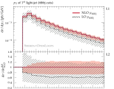
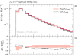
Figure 8: Distribution in the $p_{\mathrm{T}}$ of the leading light jet for $pp\to t\bar{t}b\bar{b}j$ at 13 TeV in the ttbbj phase space with acceptance cuts (11). The left figure shows LO (dashed) and NLO (solid) absolute predictions and ratios thereof. The bands correspond to seven-point scale variations. The upper frame (L1) displays the absolute $p_{\mathrm{T}}$ distribution with $\mu_{\mathrm{R}}={\mu}_{t\bar{t}b\bar{b}j}$, and the first ratio plot (L2) shows the corresponding (inverse) $K$-factor defined in (25). The other ratio plots on the left display the ratios $R_{\mathrm{(N)LO}}(\mu_{\mathrm{R}})$, defined in (26) for the scales $\mu_{\mathrm{R}}={\mu}_{gb\bar{b}}$ (L3) and ${\mu}_{\mathrm{T},\mathrm{tot}}$ (L4). Such ratios quantify shape uncertainties due to the differences between the default scale and the alternative dynamic scales. Seven-point variations in the numerator and the denominator are correlated. The right plots present normalised distributions and ratios thereof. The upper frame (R1) shows the LO and NLO normalised distributions (27) based on the default scale, with correlated seven-point variations in the numerator and denominator. The first ratio plot (R2) displays the ratio $\hat{R}_{\mathrm{(N)LO}}({\mu}_{t\bar{t}b\bar{b}j})$, which is defined in (28) and highlights the relative shape distortions induced by NLO corrections and scale variations. The last two ratio plots on the right feature the ratios $\overline{R}_{\mathrm{(N)LO}}(\mu_{\mathrm{R}})$ for $\mu_{\mathrm{R}}={\mu}_{t\bar{t}b\bar{b}j}$, ${\mu}_{gb\bar{b}}$ and ${\mu}_{\mathrm{T},\mathrm{tot}}$ at LO (R3) and NLO (R4). As defined in (29)–(30), such ratios quantify shape uncertainties associated with the kinematic dependence of the different dynamic scales.

Fig. 8 presents the distribution in the $p_{\mathrm{T}}$ of the leading light jet up to 400 GeV. The corrections to the shape of this distribution indicate excellent perturbative stability in the hard region above 150 GeV: The default scale yields a nearly constant $K$-factor around $1.65$, and the scale-variation band is also quite stable at the $\pm 20\%$ level. In the region below 150 GeV, as already observed in Fig. 7, NLO effects start affecting the $p_{\mathrm{T}}$-shape with a correction of about 25% between 150 and 50 GeV. Such effects can be attributed to Sudakov logarithms, and estimating the missing higher-order corrections via naive exponentiation, we expect residual shape uncertainties below 5% at NLO.

Comparing predictions based on the default scale and the other dynamic scales, in L3–L4 we observe normalisation differences at the level of $10$–$15$%, which are compatible with the NLO scale-variation band in L2. These differences are very stable with respect to correlated factor-two scale variations as defined in (29): at LO such variations cancel almost exactly, and also the NLO bands in L3–L4 are suppressed at the level of 5% or less. Comparing normalised distributions with different dynamic scales in R3–R4, we see that LO shapes (and their seven-point variations) are almost identical, with only few-percent differences between ${\mu}_{\mathrm{T},\mathrm{tot}}$ and the $H_{\mathrm{T}}$-independent scales. The nominal NLO predictions based on the various scales feature a similarly high level of agreement (see R4). However, similarly as in R2, factor-two variations lead to shape distortions at the 20% level. Such distortions shift the shape of the distributions in the region below 150 GeV, and are compensated by an opposite, but $p_{\mathrm{T}}$-independent shift in the hard region. In general, the suppression of shape effects at LO demonstrates the importance of NLO predictions for a more realistic assessment of shape uncertainties.

The non-negligible NLO shape effects observed in Fig. 8 are a specific feature of the jet-$p_{\mathrm{T}}$ distribution in the vicinity of the cut, while other distributions that involve the leading light jet are typically more stable.

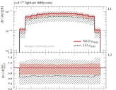
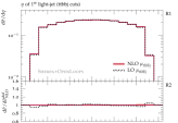
Figure 9: Pseudo-rapidity of the leading light jet. Same setup and plots as in Fig. 8.

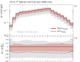
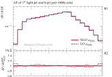
Figure 10: $\Delta R$ between the light jet and the $b$-jet pair. Same setup and plots as in Fig. 8.

This is illustrated in Figures 9–10 where we present the distributions in the pseudo-rapidity of the leading jet and in its $\Delta R$ separation with respect to the leading $b$-jet. For these observables, NLO corrections and uncertainties correspond to the ones of the integrated cross section and depend only very weakly on the jet kinematics. In fact, as can be seen from the ratio plots R2–R4, the shape of such distributions turns out to be stable at the percent level with respect of seven-point variations and differences between dynamic scales.

In general, as found in Figures 8–10 and in various other observables not shown here, distributions in the leading light jet can be controlled with typical normalisation uncertainties of order 20% and shape uncertainties of order 10% or below.

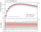
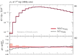
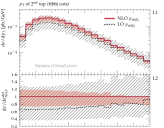
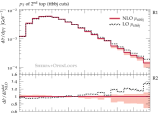
Figure 11: $p_{\mathrm{T}}$ of the harder top. Same setup and plots as in Fig. 8.

Figure 12: $p_{\mathrm{T}}$ of the softer top. Same setup and plots as in Fig. 8.

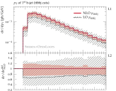
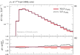
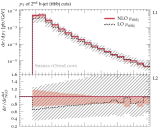
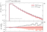
Figure 13: $p_{\mathrm{T}}$ of the first $b$-jet. Same setup and plots as in Fig. 8.

Figure 14: $p_{\mathrm{T}}$ of the second $b$-jet. Same setup and plots as in Fig. 8.

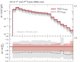
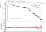
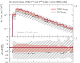
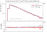
Figure 15: $\Delta R$ between the two $b$-jets. Same setup and plots as in Fig. 8.

Figure 16: Invariant mass of the $b$-jet pair. Same setup and plots as in Fig. 8.

In Figures 12–16 we present distributions in the top-quark and $b$-jet kinematics. For the transverse momentum of the harder top quark, shown in Fig. 12, we find that NLO corrections and scale variations are very stable, the only exception being a NLO shape correction of about $15\%$ in the region below 50 GeV, where the cross section is strongly suppressed. For the $p_{\mathrm{T}}$ of the softer top quark, shown in Fig. 12, NLO corrections feature a moderate, but more significant kinematic dependence. In particular, the $K$-factor goes down from about 1.5 in the bulk of the distribution to 1.2 in the tail, while seven-point scale variations lead to a similarly large shape distortion in the tail (see R2, R4). This behaviour is qualitatively quite similar to the Sudakov effects observed in the soft region of the jet-$p_{\mathrm{T}}$ distribution in Fig. 8. It can be attributed to the fact that requiring two very hard top quarks restricts the available phase for additional radiation, confining the light jet into the soft region close to the 50 GeV threshold.

The distributions in the $p_{\mathrm{T}}$ of the harder and softer $b$-jets, shown in Figures 14–14, feature a qualitatively very similar behaviour as the corresponding top-quark distributions. In the case of the harder $b$-jet $p_{\mathrm{T}}$, NLO corrections and scale uncertainties depend rather weakly on $p_{\mathrm{T}}$ (although more significantly than for the harder top quark), while the distribution in the $p_{\mathrm{T}}$ of the softer $b$-jet features strong NLO effects, which are most likely due to Sudakov logarithms.

Finally, in Figures 16–16 we show the $\Delta R$ separation and the invariant-mass distribution of the $b$-jet pair. For these observables, as far as the default scale and the scale $\mu_{\mathrm{R}}={\mu}_{\mathrm{T},\mathrm{tot}}$ are concerned, NLO corrections and variations feature very little kinematic dependence, with percent-level shape differences. On the contrary, the dynamic scale $\mu_{\mathrm{R}}={\mu}_{gb\bar{b}}$ leads to a very different shape in the tail of the $\Delta R_{bb}$ distribution, with deviations that reach $-45\%$ at LO and remain as important as $-30\%$ at NLO. A similar, although less dramatic trend is observed also in the tail of the invariant-mass distribution, which is clearly correlated to the tail of the $\Delta R_{bb}$ distribution. These effects are most pronounced at $\Delta R_{bb}>\pi$, where the two $b$-jets are emitted in opposite hemispheres. In this region, the main mechanism of $t\bar{t}b\bar{b}$ production via final-state $g\to b\bar{b}$ splittings (see Fig. 3a) is strongly suppressed, and the leading role is played by topologies with initial-state $g\to b\bar{b}$ splittings (see Fig. 3b in this paper and Fig.6 in Jezo:2018yaf ). The latter are maximally enhanced at $E_{\mathrm{T},b}\ll m_{bb}$, and their characteristic virtualities of order $E_{\mathrm{T},b}$ are correctly reflected in the definition of the scales ${\mu}_{t\bar{t}b\bar{b}j}$ and ${\mu}_{\mathrm{T},\mathrm{tot}}$. Instead, the term $m_{b\bar{b}}$ in (5) renders ${\mu}_{gb\bar{b}}$ unnaturally hard, leading to an unphysical suppression of the tails. It is clear that this behaviour cannot be regarded as a theoretical uncertainty, but should simply be taken as an indication that the scale ${\mu}_{gb\bar{b}}$, which was designed to account for final-state $g\to b\bar{b}$ splittings, is not applicable to initial-state $g\to b\bar{b}$ splittings. On the contrary, the scales ${\mu}_{t\bar{t}b\bar{b}j}$ and ${\mu}_{\mathrm{T},\mathrm{tot}}$ turn out to be well behaved for both kinds of splittings.

5.2 Recoil observables

As pointed out in the introduction, the accuracy of NLO Monte Carlo simulations of $t\bar{t}b\bar{b}$ production plays a key role in $t\bar{t}H$ analyses. In this context, it was recently observed that the modelling of recoil effect by the parton shower may be a dominant source of uncertainty (see e.g. talkPozzoriniHXSWGDec18 ; talkPozzoriniHXSWGJun19 ). This is not surprising, given that every second $t\bar{t}b\bar{b}$ event is accompanied by QCD radiation with $p_{\mathrm{T}}>50\,$GeV (see Table 3). In fact, away from the collinear regions, the recoil prescriptions used by parton showers can easily lead to unphysical momentum shifts of the order of 10 GeV and beyond. In the case of $b$-jets the effects of recoil mismodelling can be quite significant. In particular, shifts in the transverse momentum of the second $b$-jet can easily result in sizeable migration effects from the strongly populated region with $N^{\mathrm{min}}_{b}=1$ to the less populated $N^{\mathrm{min}}_{b}=2$ region.

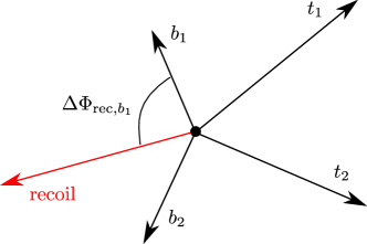
Figure 17: Sketch of the azimuthal angular correlation $\Delta\phi_{\mathrm{rec},X}$ between individual objects of the $t\bar{t}b\bar{b}$ system and its recoil. See (31)–(32).

In this context, the accurate description of QCD radiation provided by the calculation of $pp\to t\bar{t}b\bar{b}j$ at NLO can be exploited as a benchmark to test the modelling of recoil effects in $t\bar{t}b\bar{b}$ Monte Carlo simulations. With this motivation in mind, we study the azimuthal angular correlations talkPozzoriniHXSWGJun19

$$\Delta\phi_{\mathrm{rec},X} = \Delta\phi\left(\vec{p}_{\mathrm{T},\mathrm{rec}},\vec{p}_{\mathrm{T},X}\right)$$ (31)

between the transverse momentum of the recoil,

$$\vec{p}_{\mathrm{T},\mathrm{rec}} = \sum_{i=t_{1},t_{2},b_{1},b_{2}}\vec{p}_{\mathrm{T},i}\,,$$ (32)

and the various objects $X$ of the $t\bar{t}b\bar{b}$ system, i.e. the harder and softer top quarks ($t_{1},t_{2}$) and the harder and softer $b$-jets ($b_{1},b_{2}$), as well as the top-quark and the $b$-jet pairs. These angular observables, sketched in Fig. 17, reveal whether the respective object $X$ absorbs a significant fraction of the QCD recoil through the presence (or absence) of peaks at $\Delta\phi_{\mathrm{rec},X}=\pm\pi$.

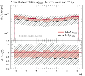
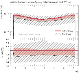
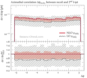
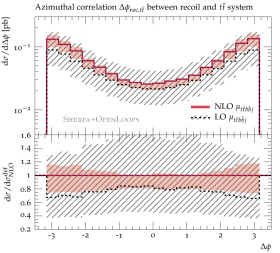
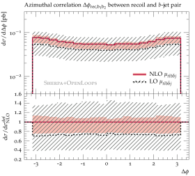
Figure 18: Distributions in the azimuthal angular separation $\Delta\phi_{\mathrm{rec},X}$ between individual objects $X$ of the $t\bar{t}b\bar{b}$ system and its recoil. See (31)–(32). The left column shows the angular correlations between the recoil and the top-quark objects $X=t_{1},t_{2},t_{1}t_{2}$, where $t_{1}t_{2}$ denotes the top-pair system. Corresponding observables for $b$-jet objects, $X=b_{1},b_{2},b_{1}b_{2}$, are shown in the right column. Same setup and plots as in Fig. 7.

In Fig. 18 we present LO and NLO predictions for the azimuthal correlations between the recoil and the various top-quark and $b$-jet objects. For these observables we focus on the default scale, $\mu_{\mathrm{R}}={\mu}_{t\bar{t}b\bar{b}j}$, with seven-point variations. The absolute distributions in the upper frames indicate a very clear pattern: the recoil is preferentially absorbed by the harder top quark, and consequently also by the $t\bar{t}$ system, while the softer top quark and the $b$-jets feature only weak angular correlations with respect to the recoil. More precisely, in the case of the harder top, at $\Delta\phi=\pm\pi$ the cross section is almost five times larger as compared to the central region, while in the case of the harder (softer) $b$-jet this enhancement goes down to about 50% (20%). Thus it should be clear that naive shower models that distribute the recoil in a democratic way may lead to a significant mismodelling of the $b$-jet kinematics. Concerning the accuracy of NLO predictions in Fig. 18, we observe that all distributions are quite stable wrt to NLO corrections and scale variations. The most significant shape effects show up in the case of top-quark observables, where scale uncertainties can shift the level of the recoil peak by 15–20%, while for $b$-jets the flatness of the azimuthal correlations is remarkably stable with respect to higher-order effects.

These results demonstrate that fixed-order NLO predictions for $pp\to t\bar{t}b\bar{b}j$ can be used as a precision benchmark to validate the modelling of recoil effects in Monte Carlo simulations of $t\bar{t}b\bar{b}$ production.

6 Tuning of QCD scale choice in $\boldsymbol{t\bar{t}b\bar{b}}$ production

In the literature on $pp\to t\bar{t}b\bar{b}$ at NLO, the usage of dynamic scales of type $\mu_{\mathrm{R}}={\mu}_{t\bar{t}b\bar{b}}$ (4) has been advocated on the basis of the moderate size of the resulting NLO correction factor, $K=\sigma_{\mathrm{NLO}}/\sigma_{\mathrm{LO}}$. However, as pointed out in Jezo:2018yaf , the smallness of the observed $K$-factor was largely due to the usage of a rather high LO value of $\alpha_{\mathrm{S}}$ as input for $\sigma_{\mathrm{LO}}$, while using the same $\alpha_{\mathrm{S}}$ in $\sigma_{\mathrm{LO}}$ and $\sigma_{\mathrm{NLO}}$ results in a correction factor as large as $K\simeq 1.9$ Jezo:2018yaf . The lack of perturbative convergence, reflected by this large $K$-factor, may simply be the consequence of the fact that $\mu_{\mathrm{R}}={\mu}_{t\bar{t}b\bar{b}}$ is a suboptimal choice. At the same time, it may also be the origin of the discrepancies between NLOPS simulations of $t\bar{t}b\bar{b}$ production talkPozzoriniTOP2018 . In fact, when matrix elements at NLO are matched to parton showers, the spectrum of the hardest QCD emission receives uncontrolled corrections of order $(K-1)=\mathcal{O}(\alpha_{\mathrm{S}})$. Such effects are formally beyond NLO, but for $K\gg 1$ they can lead to sizeable distortions of the radiation spectrum talkPozzoriniTOP2018 .

In the light of these observations, and given the strong scale dependence of the $t\bar{t}b\bar{b}$ $K$-factor, it is clear that a relatively mild reduction of the nominal scale would automatically lead to a smaller $K$-factor and, possibly, also to an improved behaviour of NLO matched simulations. However, the large $t\bar{t}b\bar{b}$ $K$-factor may also be due to large higher-order effects that are not related to the choice of $\mu_{\mathrm{R}}$. In this case, a reduction of the $K$-factor via $\mu_{\mathrm{R}}$ rescaling would only give a misleading impression of perturbative convergence without curing any problem. These considerations raise the question whether a reduction of the $t\bar{t}b\bar{b}$ $K$-factor through a smaller choice of $\mu_{\mathrm{R}}$ may be supported through solid theoretical arguments. Generic considerations based on naturalness and perturbative convergence point towards a reduction of the standard $t\bar{t}b\bar{b}$ scale choice by a factor $1/2$ to $1/3$ talkPozzoriniTOP2018 . However, only the knowledge of the next perturbative order can shed full light on the goodness of a scale choice, i.e. on its effectiveness in capturing the dominant higher-order effects. In the case at hand, the $t\bar{t}b\bar{b}$ scale choice could be tuned based on the requirement that

$$\sigma^{t\bar{t}b\bar{b}}_{\mathrm{NLO}}(\mu^{\mathrm{opt}}_{\mathrm{R}},\mu^{\mathrm{opt}}_{\mathrm{F}}) \overset{!}{=} \sigma^{t\bar{t}b\bar{b}}_{\mathrm{NNLO}}(\mu_{\mathrm{R}},\mu_{\mathrm{F}})\,,$$ (33)

i.e. by optimising the choice of the scales $\mu^{\mathrm{opt}}_{\mathrm{R},\mathrm{F}}$ in such a way that NLO $t\bar{t}b\bar{b}$ predictions match NNLO ones. However, the required NNLO calculation is completely out of reach. Nonetheless, the NLO corrections to $pp\to t\bar{t}b\bar{b}j$ presented in this paper represent one of the building blocks of $t\bar{t}b\bar{b}$ production at NNLO, and as such they can provide useful insights on how to improve the $t\bar{t}b\bar{b}$ scale choice. The idea is that the condition (33) can be imposed at the level of the jet-radiation spectrum by requiring

$$\frac{\mathrm{d}\sigma^{t\bar{t}b\bar{b}}_{\mathrm{NLO}}}{\mathrm{d}p_{\mathrm{T},j}}(\mu^{\mathrm{opt}}_{\mathrm{R}},\mu^{\mathrm{opt}}_{\mathrm{F}}) \overset{!}{=} \frac{\mathrm{d}\sigma^{t\bar{t}b\bar{b}}_{\mathrm{NNLO}}}{\mathrm{d}p_{\mathrm{T},j}}(\mu_{\mathrm{R}},\mu_{\mathrm{F}})\,=\,\frac{\mathrm{d}\sigma^{t\bar{t}b\bar{b}j}_{\mathrm{NLO}}}{\mathrm{d}p_{\mathrm{T},j}}(\mu_{\mathrm{R}},\mu_{\mathrm{F}})\,.$$ (34)

With other words, the scale choice can be tuned in such a way that the tree-level description of the jet-$p_{\mathrm{T}}$ spectrum that results from the $t\bar{t}b\bar{b}$ NLO calculation matches the more precise prediction of the $t\bar{t}b\bar{b}j$ NLO calculation. Contrary to (33), this procedure cannot guarantee the correct description of higher-order effects at the level of the inclusive $t\bar{t}b\bar{b}$ cross section. Nonetheless it is attractive for at least two reasons. First, tuned $t\bar{t}b\bar{b}$ NLO predictions will guarantee a much more accurate description of the jet-$p_{\mathrm{T}}$ spectrum, which is known to play a critical role in Monte Carlo simulations. Second, the shape of the jet-$p_{\mathrm{T}}$ spectrum can be used to judge the quality of the matching procedure (34), and the general consistency of the procedure can be validated by comparing various other jet observables.

The results of this tuning procedure are presented in Fig. 19, where we show the distribution in the $p_{\mathrm{T}}$ of the hardest light jet, and in the invariant masses of the systems formed by the hardest light jet in combination with the leading or the subleading $b$-jet. The tuning is carried out through a constant rescaling of the standard $t\bar{t}b\bar{b}$ scale choice,

$$(\mu_{\mathrm{R}},\mu_{\mathrm{F}}) = (\kappa\,{\mu}_{t\bar{t}b\bar{b}},\kappa\,\frac{H_{\mathrm{T}}}{2})\,,$$ (35)

such as to match NLO predictions for the integrated ttbbj cross section based on the default scale ${\mu}_{t\bar{t}b\bar{b}j}$. To be conservative, we have compared two possible ways of tuning the $t\bar{t}b\bar{b}$ scale. In the first approach, the rescaled $t\bar{t}b\bar{b}$ NLO predictions are matched to nominal $t\bar{t}b\bar{b}j$ NLO predictions, whereas in the second approach the tuning is done by matching the average values of the respective seven-point variation bands. The outcome of these two matching prescriptions is shown in the left and right columns of Fig. 19. Matching nominal predictions leads to a reduction of the default $t\bar{t}b\bar{b}$ scale by a factor $\kappa=1/1.6$, whereas matching the scale-variation bands in a symmetric way requires a significantly smaller rescaling, $\kappa=1/1.14$. This large difference is mainly due to the strong asymmetry of the factor-two variation band of the tree-level prediction, i.e. $pp\to t\bar{t}b\bar{b}$ at NLO. In this respect, we note that such asymmetry is mainly due to the logarithmic nature of the scale dependence (13). Thus the asymmetry of the LO band would largely disappear on logarithmic scale, and the prescriptions based on the central scale and the average of the bands would be significantly closer to each other.

For all considered jet observables we find that both tuning scenarios lead to a very good agreement, not only in the normalisation, but also at the level of shapes. The findings of this analysis support a reduction of the standard $t\bar{t}b\bar{b}$ scale (35) by up to a factor $\kappa\sim 1/1.6$. In the ttbb ​(ttb) phase space, $\kappa=1/1.6$ corresponds to a reduction of the $t\bar{t}b\bar{b}$ $K$-factor from 1.80 (1.92) to 1.51 (1.62) and an increase of the nominal $t\bar{t}b\bar{b}$ cross section by 18% (21%).

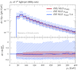
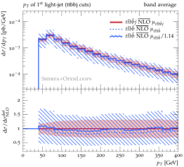
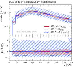
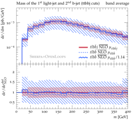
Figure 19: Distributions in the $p_{\mathrm{T}}$ of the leading jet and the mass of light-jet–$b$-jet systems in the ttbbj phase space. Comparison of NLO $t\bar{t}b\bar{b}j$ predictions with default scale choice, $(\mu_{\mathrm{R}},\mu_{\mathrm{F}})=({\mu}_{t\bar{t}b\bar{b}j},H_{\mathrm{T}}/2)$, to NLO $t\bar{t}b\bar{b}$ predictions with $(\mu_{\mathrm{R}},\mu_{\mathrm{F}})=(\kappa\,{\mu}_{t\bar{t}b\bar{b}},\kappa\,H_{\mathrm{T}}/2)$. In the left plots, the reference curves for the matching procedure (solid, labelled NLO) correspond to the above central scales, and the applied rescaling factor is $\kappa=1/1.6$. In the right plots, the reference curves (solid, labelled $\overline{\mathrm{NLO}}$) are the average values of the scale-variation bands, and $\kappa=1/1.14$. The blue dashed curves indicate the position of the NLO $t\bar{t}b\bar{b}$ reference prediction before tuning, while all other NLO $t\bar{t}b\bar{b}$ predictions and scale-variation bands correspond to the tuned scales.

7 Summary

Measurements of $t\bar{t}H(b\bar{b})$ production at the LHC require very accurate theoretical simulations of the irreducible $t\bar{t}b\bar{b}$ background. To address the dominant sources of systematic uncertainties, which stem from the modelling of QCD radiation in $t\bar{t}b\bar{b}$ events, we have presented a calculation of $t\bar{t}b\bar{b}$ production in association with one extra jet at NLO QCD.

To carry out this non-trivial calculation we used OpenLoops 2 in combination with the Sherpa and Munich Monte Carlo frameworks. Technically, the calculation of the required $2\to 5$ one-loop amplitudes has confirmed that the new algorithms implemented in OpenLoops 2 can tackle multi-particle and multi-scale problems with very high CPU efficiency and numerical stability.

We have discussed $pp\to t\bar{t}b\bar{b}j$ at the 13 TeV LHC with emphasis on the effects of NLO corrections and scale uncertainties. To this end, we have studied conventional factor-two rescalings, as well as variations of the kinematic dependence of dynamic scales. In order to disentangle normalisation and shape uncertainties in a transparent way, we have proposed to compare dynamic scales upon alignment of the NLO maxima of the respective scale-variation curves.

In general, the typical level of scale uncertainties in $pp\to t\bar{t}b\bar{b}j$ at NLO is $20$–$30$% for integrated cross sections and below 10% in the shapes of distributions. The calculation at hand can thus be used as a precision benchmark to validate the modelling of QCD radiation in Monte Carlo generators of $t\bar{t}b\bar{b}$ production. With this motivation in mind, we have presented NLO predictions for various azimuthal correlations that provide a transparent picture of the effects of the recoil of QCD radiation on the different objects of the $t\bar{t}b\bar{b}$ system.

Finally, we have discussed the issue of the large NLO $K$-factor observed in inclusive NLO calculations of $t\bar{t}b\bar{b}$ production, and we have addressed the question of whether it is justified to reduce this $K$-factor through ad-hoc scale choices. In this respect we have argued that the NLO corrections to $pp\to t\bar{t}b\bar{b}j$ entail information on $pp\to t\bar{t}b\bar{b}$ beyond NLO, which can be exploited to identify an optimised scale choice. Specifically, we have proposed the idea of adjusting the nominal $t\bar{t}b\bar{b}$ scale choice such as to match the jet emission rate predicted by $pp\to t\bar{t}b\bar{b}j$ at NLO. This improved scale choice leads to a reduction of the $t\bar{t}b\bar{b}$ $K$-factor, and is also expected to attenuate theoretical uncertainties in the context of NLO matching to parton showers.

- (1) ATLAS collaboration, Search for the standard model Higgs boson produced in association with top quarks and decaying into a pair in collisions at = 13 TeV with the ATLAS detector, Phys. Rev. D97 (2018) 072016 [1712.08895].
- (2) CMS collaboration, Search for production in the decay channel with leptonic decays in proton-proton collisions at TeV, JHEP 03 (2019) 026 [1804.03682].
- (3) CMS collaboration, Measurement of production in the decay channel in of proton-proton collision data at , CMS-PAS-HIG-18-030 (2019) .
- (4) HL/HE WG2 group collaboration, Higgs Physics at the HL-LHC and HE-LHC, 1902.00134.
- (5) CMS collaboration, Measurements of cross sections in association with jets and inclusive jets and their ratio using dilepton final states in pp collisions at = 13 TeV, Phys. Lett. B776 (2018) 355 [1705.10141].
- (6) ATLAS collaboration, Measurements of inclusive and differential fiducial cross-sections of production with additional heavy-flavour jets in proton-proton collisions at = 13 TeV with the ATLAS detector, JHEP 04 (2019) 046 [1811.12113].
- (7) CMS collaboration, Measurement of the production cross section in the all-jet final state in collisions at , CMS-PAS-TOP-18-011 (2019) .
- (8) A. Bredenstein, A. Denner, S. Dittmaier and S. Pozzorini, NLO QCD corrections to at the LHC, Phys. Rev. Lett. 103 (2009) 012002 [0905.0110].
- (9) G. Bevilacqua, M. Czakon, C. G. Papadopoulos, R. Pittau and M. Worek, Assault on the NLO Wishlist: , JHEP 09 (2009) 109 [0907.4723].
- (10) A. Bredenstein, A. Denner, S. Dittmaier and S. Pozzorini, NLO QCD Corrections to Top Anti-Top Bottom Anti-Bottom Production at the LHC: 2. full hadronic results, JHEP 03 (2010) 021 [1001.4006].
- (11) F. Cascioli, P. Maierhöfer, N. Moretti, S. Pozzorini and F. Siegert, NLO matching for production with massive -quarks, Phys. Lett. B734 (2014) 210 [1309.5912].
- (12) T. Ježo, J. M. Lindert, N. Moretti and S. Pozzorini, New NLOPS predictions for -jet production at the LHC, Eur. Phys. J. C78 (2018) 502 [1802.00426].
- (13) M. V. Garzelli, A. Kardos and Z. Trocsanyi, hadroproduction at NLO accuracy matched with parton shower, PoS EPS-HEP2013 (2013) 253.
- (14) M. V. Garzelli, A. Kardos and Z. Trocsanyi, Hadroproduction of final states at LHC: predictions at NLO accuracy matched with Parton Shower, JHEP 03 (2015) 083 [1408.0266].
- (15) J. Alwall, R. Frederix, S. Frixione, V. Hirschi, F. Maltoni et al., The automated computation of tree-level and next-to-leading order differential cross sections, and their matching to parton shower simulations, JHEP 1407 (2014) 079 [1405.0301].
- (16) J. Bellm et al., Herwig 7.0/Herwig++ 3.0 release note, Eur. Phys. J. C76 (2016) 196 [1512.01178].
- (17) LHC Higgs Cross Section Working Group collaboration, Handbook of LHC Higgs Cross Sections: 4. Deciphering the Nature of the Higgs Sector, 1610.07922.
- (18) F. Buccioni, “NLO predictions for production in association with a light-jet at the LHC.” https://indico.cern.ch/event/662485/contributions/3074074/ (talk given at QCD@LHC 2018).
- (19) F. Buccioni, “NLO predictions for production in association with a light-jet at the LHC.” https://indico.cern.ch/event/694599/contributions/3142622/ (talk given at the 7th International Workshop on High Precision for Hard Processes (HP2 2018)).
- (20) F. Buccioni, J.-N. Lang, J. M. Lindert, P. Maierhöfer, S. Pozzorini, H. Zhang and M. F. Zoller, OpenLoops 2, 1907.13071.
- (21) F. Buccioni, S. Pozzorini and M. Zoller, On-the-fly reduction of open loops, Eur. Phys. J. C78 (2018) 70 [1710.11452].
- (22) F. Krauss, R. Kuhn and G. Soff, AMEGIC++ 1.0: A Matrix element generator in C++, JHEP 0202 (2002) 044 [hep-ph/0109036].
- (23) T. Gleisberg, S. Höche, F. Krauss, M. Schönherr, S. Schumann, F. Siegert and J. Winter, Event generation with SHERPA 1.1, JHEP 02 (2009) 007 [0811.4622].
- (24) T. Gleisberg and S. Höche, Comix, a new matrix element generator, JHEP 12 (2008) 039 [0808.3674].
- (25) T. Gleisberg and F. Krauss, Automating dipole subtraction for QCD NLO calculations, Eur. Phys. J. C53 (2008) 501 [0709.2881].
- (26) S. Catani and M. H. Seymour, A general algorithm for calculating jet cross sections in NLO QCD, Nucl. Phys. B485 (1997) 291 [hep-ph/9605323].
- (27) S. Catani, S. Dittmaier, M. H. Seymour and Z. Trocsanyi, The dipole formalism for next-to-leading order QCD calculations with massive partons, Nucl. Phys. B627 (2002) 189 [hep-ph/0201036].
- (28) F. Cascioli, P. Maierhöfer and S. Pozzorini, Scattering Amplitudes with Open Loops, Phys.Rev.Lett. 108 (2012) 111601 [1111.5206].
- (29) A. Denner and S. Dittmaier, Scalar one-loop 4-point integrals, Nucl. Phys. B844 (2011) 199 [1005.2076].
- (30) A. Denner, S. Dittmaier and L. Hofer, COLLIER - A fortran-library for one-loop integrals, PoS LL2014 (2014) 071 [1407.0087].
- (31) A. Denner, S. Dittmaier and L. Hofer, Collier: a fortran-based Complex One-Loop LIbrary in Extended Regularizations, 1604.06792.
- (32) A. van Hameren, OneLOop: For the evaluation of one-loop scalar functions, Comput.Phys.Commun. 182 (2011) 2427 [1007.4716].
- (33) A. Denner and S. Dittmaier, Reduction of one loop tensor five point integrals, Nucl. Phys. B658 (2003) 175 [hep-ph/0212259].
- (34) A. Denner and S. Dittmaier, Reduction schemes for one-loop tensor integrals, Nucl. Phys. B734 (2006) 62 [hep-ph/0509141].
- (35) G. Ossola, C. G. Papadopoulos and R. Pittau, CutTools: a program implementing the OPP reduction method to compute one-loop amplitudes, JHEP 03 (2008) 042 [0711.3596].
- (36) G. Ossola, C. G. Papadopoulos and R. Pittau, Reducing full one-loop amplitudes to scalar integrals at the integrand level, Nucl. Phys. B763 (2007) 147 [hep-ph/0609007].
- (37) S. Actis, A. Denner, L. Hofer, J.-N. Lang, A. Scharf and S. Uccirati, RECOLA: REcursive Computation of One-Loop Amplitudes, Comput. Phys. Commun. 214 (2017) 140 [1605.01090].
- (38) A. Denner, J.-N. Lang and S. Uccirati, Recola2: REcursive Computation of One-Loop Amplitudes 2, Comput. Phys. Commun. 224 (2018) 346 [1711.07388].
- (39) C. Duhr, S. Höche and F. Maltoni, Color-dressed recursive relations for multi-parton amplitudes, JHEP 08 (2006) 062 [hep-ph/0607057].
- (40) A. Buckley, J. Butterworth, L. Lönnblad, D. Grellscheid, H. Hoeth, J. Monk, H. Schulz et al., Rivet user manual, Comput. Phys. Commun. 184 (2013) 2803 [1003.0694].
- (41) M. Cacciari and G. P. Salam, Dispelling the myth for the jet-finder, Phys.Lett. B641 (2006) 57 [hep-ph/0512210].
- (42) M. Cacciari, G. P. Salam and G. Soyez, FastJet User Manual, Eur.Phys.J. C72 (2012) 1896 [1111.6097].
- (43) M. Grazzini, S. Kallweit and M. Wiesemann, Fully differential NNLO computations with MATRIX, Eur. Phys. J. C78 (2018) 537 [1711.06631].
- (44) F. Cascioli, S. Kallweit, P. Maierhöfer and S. Pozzorini, A unified NLO description of top-pair and associated Wt production, Eur. Phys. J. C74 (2014) 2783 [1312.0546].
- (45) S. Catani, S. Devoto, M. Grazzini, S. Kallweit, J. Mazzitelli and H. Sargsyan, Top-quark pair hadroproduction at next-to-next-to-leading order in QCD, Phys. Rev. D99 (2019) 051501 [1901.04005].
- (46) S. Catani, S. Devoto, M. Grazzini, S. Kallweit and J. Mazzitelli, Top-quark pair production at the LHC: Fully differential QCD predictions at NNLO, JHEP 07 (2019) 100 [1906.06535].
- (47) NNPDF collaboration, Parton distributions for the LHC Run II, JHEP 04 (2015) 040 [1410.8849].
- (48) A. Buckley, J. Ferrando, S. Lloyd, K. Nordström, B. Page, M. Rüfenacht, M. Schönherr et al., LHAPDF6: parton density access in the LHC precision era, Eur. Phys. J. C75 (2015) 132 [1412.7420].
- (49) M. Cacciari, G. P. Salam and G. Soyez, The anti- jet clustering algorithm, JHEP 04 (2008) 063 [0802.1189].
- (50) S. Pozzorini, “ recent theory developments.” https://indico.cern.ch/event/740110/contributions/3192779/ (talk given at the 15th Workshop of the LHC Higgs Cross Section Working Group).
- (51) S. Pozzorini, “Heavy flavour backgrounds in .” https://indico.cern.ch/event/827858/contributions/3481144/ (talk given at the HXSWG meeting on “Parton Shower Uncertainties in Higgs Measurements”).
- (52) S. Pozzorini, “Theory progress on background.” https://indico.cern.ch/event/690229/contributions/2979729/ (talk given at the 11th International Workshop on Top Quark Physics (TOP2018)).