Conditional independence testing: a predictive perspective

Marco Henrique de Almeida Inácio    Rafael Izbicki    Rafael Bassi Stern

Abstract

Conditional independence testing is a key problem required by many machine learning and statistics tools. In particular, it is one way of evaluating the usefulness of some features on a supervised prediction problem. We propose a novel conditional independence test in a predictive setting, and show that it achieves better power than competing approaches in several settings. Our approach consists in deriving a p-value using a permutation test where the predictive power using the unpermuted dataset is compared with the predictive power of using dataset where the feature(s) of interest are permuted. We conclude that the method achives sensible results on simulated and real datasets.

Keywords:

Supervised learning Conditional independence testing Hypothesis test

1 Introduction

Conditional independence testing is a key problem required by many machine learning and statistics tools, including Bayesian networks jensen1996 (14, 4), time series DIKS20061647 (7) , causal inference spirtes2000 (21, 17) and feature selection koller1996 (16).

Unfortunately, it is not possible to design conditional independence tests that are powerful against all points in the alternative hypothesis shah2018 (20). Nevertheless, this issue can be partially addressed by assuming additional structure on the data distribution. Indeed, various conditional independence methods take advantage of specific settings to obtain improved power for alternatives of interest; see, for instance, doran2014 (8, 19, 1, 5) and references therein.

In this work we are interested in testing conditional independence as a way of evaluating the usefulness of some features on a supervised prediction problem. More precisely, let ${\mathbf{X}}^{S}\subset(X_{1},\ldots,X_{p})$ be a subset of the features. Our goal is to test if ${\mathbf{X}}^{S}$ is independent of the label $Y$ conditionally on ${\mathbf{X}}^{S^{c}}$, the remaining variables, i.e, we wish to test the hypothesis $H_{0}:{\mathbf{X}}^{S}\bot Y|{\mathbf{X}}^{S^{c}}$.

This is setting is closely connected to the literature of designing effective variable importance measures, in which the goal is to design indices that can be used to rank features according to how useful they are for predicting $Y$. A popular measure of variable importance was designed by breiman2001 (3), but several alternative procedures are also available; see, for instance, strobl2008 (22, 9) and references therein. Conditional independence testing is distinct from designing importance measures in the sense that its goal is not to quantify how informative a given feature is, but instead to answer the question: “is this feature relevant?".

In this work we propose an approach to answer this question that consists in comparing the performance of two prediction methods: the first is trained using all features, while the second uses noise instead of the variables $S$. We show that our method yields a formal statistical hypothesis that approximately controls the significance level, and that it achieves considerable power against relevant alternative hypotheses.

Our work is related to watson2019 (23), who also compare the risk of two prediction methods in order to test $H_{0}$. The main difference between these methods is that we use a permutation test-based statistic to compute p-values (see Section 3 for further details). We show that this leads to substantial gain of power in several settings, and also a better control of type I error probabilities, especially for smaller sample sizes.

The remaining of this paper is organized as follows. Section 2 introduces COINP, our approach to test conditional independence. Section 3 contains experiments for comparing COINP with other approaches while Section 4 presents an illustrative example of applying the method to a real world dataset together the classical importance measure obtained from random forests. Section 5 concludes the paper with final remarks.

2 Conditional Independence Predictive Test (COINP)

2.1 Notation and problem setting

Let $\mathcal{X}$ denote the feature space and $\mathcal{Y}$ the label space. The observed data is ${\mathbb{Z}}=({\mathbb{X}},{\mathbf{Y}})$, where ${\mathbb{X}}\in\mathcal{X}^{n}$ is a $n\times p$ feature matrix and ${\mathbf{Y}}\in\mathcal{Y}^{n}$ is the label vetor. We assume that the observations ${\mathbf{z}}_{i}=({\mathbf{x}}_{i},y_{i})$, $i=1,\ldots,n$, are independent and identically distributed. Let ${\mathbf{X}}^{S}\subset(X_{1},\ldots,X_{p})$ be a subset of the features. Our goal is to test if ${\mathbf{X}}^{S}$ is independent of $Y$ conditionally on ${\mathbf{X}}^{S^{c}}$, the remaining variables, i.e, we wish to test the hypothesis $H_{0}:{\mathbf{X}}^{S}\bot Y|{\mathbf{X}}^{S^{c}}$.

We denote by $\mathcal{F}:=\{f:\mathcal{X}\longrightarrow\mathcal{Y}\}$ the space of all mappings from features to outcomes (i.e., all prediction functions), and by $\mathcal{Z}$ the set of all datasets. A prediction method (e.g., neural networks or random forests) is a function in the space $\mathcal{A}=\{a:\mathcal{Z}\longrightarrow\mathcal{F}\}$. We denote a loss function by $L:{\mathcal{Y}}\times{\mathcal{Y}}\longrightarrow\mathbb{R}$. The risk of a prediction function $f\in{\mathcal{F}}$ is $R(f):={\mathbb{E}}[L(f({\mathbf{X}}),Y)]$. We denote by

$$\widehat{R}(f,\tilde{{\mathbb{Z}}}):=\frac{1}{n}\sum_{i=1}^{n}L(f(\tilde{{\mathbf{x}}}_{i}),\tilde{y}_{i})$$

the estimate of the risk of $f\in{\mathcal{F}}$ based on a holdout dataset $\tilde{{\mathbb{Z}}}$ of size $n$ (i.e., a dataset not used for obtaining $f$).

The Conditional Independence Predictive Test (COINP) requires one to randomly permuting the rows of ${\mathbb{X}}$ associated to the features $S$. This procedure is illustrated in Figure 1 for an example with $S=\{X_{3}\}$. For every $j=1,\ldots,B$, denote by ${\mathbb{Z}}^{\pi_{j}}$ the $j$-th dataset obtained by performing this procedure on ${\mathbb{Z}}$, and let ${\mathbf{x}}^{\pi_{j}}_{i}$ be the $i$-th observation of such dataset. Similarly, we denote by $\tilde{{\mathbb{Z}}}^{\pi_{j}}$ the $j$-th permutation of the holdout set $\tilde{{\mathbb{Z}}}$. Table 1 summarizes the notation used in this paper.

$${\mathbb{Z}}\hskip 5.69054pt:=\hskip 5.69054pt\begin{matrix}X_{1}&X_{2}&X_{3}&Y\\ \blacktriangle&\blacklozenge&{\color[rgb]{0,0,1}\blacksquare}&\bigstar\\ \blacksquare&\blacktriangle&{\color[rgb]{0,0,1}\blacktriangle}&\bigstar\\ \blacktriangle&\bigstar&{\color[rgb]{0,0,1}\bigstar}&\blacksquare\\ \blacksquare&\blacklozenge&{\color[rgb]{0,0,1}\blacktriangle}&\blacklozenge\\ \bigstar&\blacklozenge&{\color[rgb]{0,0,1}\blacktriangledown}&\blacksquare\\ \bigstar&\blacktriangledown&{\color[rgb]{0,0,1}\bigstar}&\blacktriangledown\\ \end{matrix}\hskip 22.76219pt{{\Rightarrow}}\hskip 22.76219pt\begin{matrix}X_{1}&X_{2}&X_{3}&Y\\ \blacktriangle&\blacklozenge&{\color[rgb]{0,0,1}\blacktriangle}&\bigstar\\ \blacksquare&\blacktriangle&{\color[rgb]{0,0,1}\blacksquare}&\bigstar\\ \blacktriangle&\bigstar&{\color[rgb]{0,0,1}\bigstar}&\blacksquare\\ \blacksquare&\blacklozenge&{\color[rgb]{0,0,1}\bigstar}&\blacklozenge\\ \bigstar&\blacklozenge&{\color[rgb]{0,0,1}\blacktriangle}&\blacksquare\\ \bigstar&\blacktriangledown&{\color[rgb]{0,0,1}\blacktriangledown}&\blacktriangledown\\ \end{matrix}\hskip 5.69054pt=:\hskip 5.69054pt{\mathbb{Z}}^{\pi}$$

Figure 1: Permutation procedure used to test if the $X_{3}$ is independent of $Y$ conditionally on $X_{1}$ and $X_{2}$.

Table 1: Notation used in the paper.

Symbol	Meaning
${\mathbb{X}}$	$n\times p$ feature matrix
$Y$	Label vector
${\mathbb{Z}}$	Training data
$\tilde{{\mathbb{Z}}}$	Holdout data
${\mathcal{F}}$	space of all prediction functions
${\mathcal{A}}$	space of all prediction methods
$\widehat{R}(f,{\mathbb{Z}})$	Estimate of the risk of $f\in{\mathcal{F}}$ based on ${\mathbb{Z}}$
${\mathbb{Z}}^{\pi_{j}}$	$j$-th dataset with the rows of the $S$ columns of ${\mathbb{Z}}$ are randomly permuted
${\mathbf{x}}_{i}^{\pi_{j}}$	The features of the $i$-th row of ${\mathbb{Z}}^{\pi_{j}}$

2.2 Proposed method

The COINP procedure consists in testing $H_{0}$ by computing the rank of $\widehat{R}(a({\mathbb{Z}}),\tilde{{\mathbb{Z}}})$ among

$$\{\widehat{R}(a({\mathbb{Z}}^{\pi_{1}}),\tilde{{\mathbb{Z}}}^{\pi_{1}}),\ldots,\widehat{R}(a({\mathbb{Z}}^{\pi_{B}}),\tilde{{\mathbb{Z}}}^{\pi_{B}})\},$$

where $a\in{\mathcal{A}}$ is any prediction method. We then reject the null hypothesis if this statistic is small. The intuition of this procedure is that, if $H_{0}$ does not hold (i.e., if the features $S$ still have information about $Y$ even given $S^{c}$), an algorithm that uses $S$ in addition to $S^{c}$ will result in greater predictive power than one that does not use those features. Thus, permuting the rows associated with $S$ will result in a prediction function with larger risk. Hence, if $H_{0}$ does not hold, $\widehat{R}(a({\mathbb{Z}}),\tilde{{\mathbb{Z}}})$ should be smaller than most $\widehat{R}(a({\mathbb{Z}}^{\pi_{j}}),\tilde{{\mathbb{Z}}}^{\pi_{j}})$’s. On the other hand, if $H_{0}$ holds, the features ${\mathbf{X}}^{S}$ bring no additional gain in the predictive performance of $a$. It follows that the estimated risk $\widehat{R}(a({\mathbb{Z}}),\tilde{{\mathbb{Z}}})$ should be identically distributed to $\widehat{R}(a({\mathbb{Z}}^{\pi_{j}}),\tilde{{\mathbb{Z}}}^{\pi_{j}})$. It follows that the rank statistic is uniformly distributed under the null hypothesis. This justifies the following COINP procedure, which we formally state in the following definition.

Definition 1 (COINP – Conditional Independence Predictive Test)

Let $\alpha\in(0,1)$ and $a\in{\mathcal{A}}$ be a predictive method. The $\alpha$-level Conditional Independence Predictive Test consists in rejecting the null hypothesis $H_{0}:{\mathbf{X}}^{S}\bot Y|{\mathbf{X}}^{S^{c}}$ if, and only if,

$$\frac{1}{B}\sum_{j=1}^{B}{\mathbb{I}}\left(\widehat{R}(a({\mathbb{Z}}),\tilde{{\mathbb{Z}}})\geq\widehat{R}(a({\mathbb{Z}}^{\pi_{j}}),\tilde{{\mathbb{Z}}}^{\pi_{j}})\right)\leq\alpha.$$ (1)

The COINP is described in Algorithm 1. Notice that the left-hand side of Equation 1 is in fact a p-value based on a permutation test good2013 (11) .

Algorithm 1 COINP

Input: training data ${\mathbb{Z}}$, testing data $\tilde{{\mathbb{Z}}}$, prediction method $a\in{\mathcal{A}}$, loss function $L$, feature indices $S$, number of simulations $B$ Output: p-value for testing $H_{0}:{\mathbf{X}}^{S}\bot Y|{\mathbf{X}}^{S^{c}}$ 1:$f\leftarrow a({\mathbb{Z}})$ 2:$R\leftarrow\widehat{R}(f,\tilde{{\mathbb{Z}}})$ 3:for $j\in\{1,\ldots,B\}$ do 4:     Compute ${\mathbb{Z}}^{\pi_{j}}$ by randomly permuting the columns of ${\mathbb{Z}}$ associated to features $S$ 5:     $f_{j}\leftarrow a({\mathbb{Z}}^{\pi_{j}})$ 6:     Compute $\tilde{{\mathbb{Z}}}^{\pi_{j}}$ by randomly permuting the columns of $\tilde{{\mathbb{Z}}}$ associated to features $S$ 7:     $R_{j}\leftarrow\widehat{R}(f_{j},\tilde{{\mathbb{Z}}}^{\pi_{j}})$ 8:end for 9:return $|\{j:R\geq R_{j}\}|/B$

3 Experiments

3.1 Other approaches

We compare our permutation method with the following approaches.

3.1.1 Conditional Predictive Impact (CPI)

The Conditional Predictive Impact (CPI) test, introduced by watson2019 (23), consists in training two prediction methods: one on the original dataset, $f=a({\mathbb{Z}})$, and another one on a permuted dataset, $f_{1}=a({\mathbb{Z}}^{\pi_{1}})$. It then tests the one-sided null hypothesis $H_{0}:R(f,\tilde{{\mathbb{Z}}})\geq R(f_{1},\tilde{{\mathbb{Z}}}^{\pi_{1}})$ by checking if the distribution of the loss function on the original set,

$$(L(f(\tilde{{\mathbf{x}}}_{1}),\tilde{y}_{1}),\ldots,L(f(\tilde{{\mathbf{x}}}_{n}),\tilde{y}_{n}))$$

comes from a distribution with smaller average than the distribution of the loss function on the permuted test,

$$(L(f_{1}(\tilde{{\mathbf{x}}}^{\pi_{1}}_{1}),\tilde{y}_{1}),\ldots,L(f_{1}(\tilde{{\mathbf{x}}}^{\pi_{1}}_{n}),\tilde{y}_{n})).$$

In practice, we use the paired t-test to perform this comparison; see watson2019 (23) for other approaches.

3.1.2 Approximate CPI

We include a variation of CPI in which the same prediction function, $f=a({\mathbb{Z}})$, is used compute on both datasets. That is, in this version of the test, a paired t-test is used to compare the samples

$$(L(f(\tilde{{\mathbf{x}}}_{1}),\tilde{y}_{1}),\ldots,L(f(\tilde{{\mathbf{x}}}_{n}),\tilde{y}_{n}))$$

and

$$(L(f(\tilde{{\mathbf{x}}}^{\pi_{1}}_{1}),\tilde{y}_{1}),\ldots,L(f(\tilde{{\mathbf{x}}}^{\pi_{1}}_{n}),\tilde{y}_{n})).$$

This procedure is essentially the method described by breiman2008 (2) to obtain p-values for the importance measures produced by random forests, with the exception that breiman2008 (2) use a $z$-test instead.

3.1.3 Approximate COINP

A drawback of COINP is that it is computationally intensive, especially if $a$ is a slow predictive algorithm. We attempt to overcome these issues by computing the rank of $\widehat{R}(a({\mathbb{Z}}),\tilde{{\mathbb{Z}}})$ on

$$\{\widehat{R}(a({\mathbb{Z}}),\tilde{{\mathbb{Z}}}^{\pi_{1}}),\ldots,\widehat{R}(a({\mathbb{Z}}),\tilde{{\mathbb{Z}}}^{\pi_{B}})\},$$

that is, we train $a$ only once (on the original dataset). In other words, approximate COINP using the same procedure as that described in Algorithm 1, with the exception that line 4 and 5 are now replaced by $f_{j}\leftarrow f$.

3.2 Simulation study description

Next, we describe the details of the simulation study performed to evaluate the proposed method.

3.2.1 Simulation scenarios

We generate artificial datasets for our simulation study using various distributions. We restrict our comparisons to regression settings with the squared loss, $L(y,\widehat{y})=(y-\widehat{y})^{2}$, even though our method is general and can be used for classification as well. Moreover, in what follows we will always test conditional independence of a single feature, i.e., $|S|=1$.

The first and second scenarios have features that are independent of each other.

Distribution 1:

$$Y_{i}={\mathbf{X}}_{i}\beta+\epsilon$$

$$\beta=(0.7,0.16,0.39,\beta_{S},0.75)$$

$$\epsilon\sim\text{SKN}(-0.3,1.1,2)$$

$$Z_{i,j}\sim\text{SKN}(0,0.1,2),\ j=1,\ldots,5\text{ (i.i.d)}$$

$$X_{1}=|Z_{1}|^{1.3}$$

$$X_{2}=\cos(Z_{2})$$

$$X_{3}=\log(|Z_{1}Z_{3}|)$$

$$X_{4}=\log(|Z_{3}|)$$

$$X_{5}=\sqrt{|Z_{4}|}$$

$$\text{Observed input}:(X_{1},X_{2})$$

$$\text{Observed output}:Y$$

Distribution 2:

$$Y=Z\beta+\epsilon$$

$$\beta\approx(0.7,0.16,0.39,\beta_{S},0.75)$$

$$\epsilon\sim\text{SKN}(-0.3,1.1,2)$$

$$X\sim\text{SKN}(0,0.1,2)\text{ (i.i.d)}$$

$$Z_{1}=|X_{1}|^{1.3}$$

$$Z_{2}=\cos(X_{2})$$

$$Z_{3}=\log(|X_{1}X_{3}|)$$

$$Z_{4}=\log(|X_{3}|)$$

$$Z_{5}=\sqrt{|X_{4}|}$$

$$\text{Observed input}:{\mathbf{X}}$$

$$\text{Observed output}:Y$$

In the other settings, we add correlation to the features (here SKN stands for skew normal distribution with location, scale and shape parameters respectively):

Distribution 3:

$$Y_{i}={\mathbf{X}}_{i}\beta+\epsilon$$

$$\beta=(3,\beta_{S})$$

$${\mathbf{X}}_{i}\sim N(0,\Sigma)$$

$$\epsilon\sim N(0,0.5)$$

$$\Sigma_{0,0}=1$$

$$\Sigma_{0,1}=0.9$$

$$\text{Observed input}:{\mathbf{X}}$$

$$\text{Observed output}:Y$$

Distribution 4:

$$Y_{i}={\mathbf{X}}_{i}\beta+\epsilon$$

$$\beta=(3,\beta_{S})$$

$$\epsilon\sim\text{beta}(2,2)$$

$$W_{j}\sim\text{beta}(1,1)\text{ for }j\in\{1,2\}$$

$$Z\sim N(-0.5,1)$$

$${\mathbf{X}}_{i,j}=Z+W_{j}\text{ for }j\in\{1,2\}$$

$$\text{Observed input}:{\mathbf{X}}$$

$$\text{Observed output}:Y$$

For all the combinations described above, we vary $\beta_{S}$ in $\{0,0.01,0.1,0.6\}$ and the number of observations in $\{1000,10000\}$. Notice that, in all settings, $H_{0}$ holds if, and only if, $\beta_{S}=0$. Moreover, as $|\beta_{S}|$ increases, the conditional dependency of $Y$ on ${\mathbf{X}}^{S}$ also increases.

For each setting we run 200 independent tests to estimate the power of each test. We set $B=100$.

We compare three choices for the prediction function $a$:

1. Linear regression, implemented using scikit-learn Python package scikit-learn (18).

2. Feedforward neural networks. The specification of the network is as follows:

   • Optimizer: we work with the Adamax optimizer adam-optim (15) and decrease its learning rate if improvement is seen on the validation loss for a considerable number of epochs.

   • Initialization: we used the initialization method proposed by nn-initialization (10).

   • Layer activation: we chose ELU elu (6) as activation function.

   • Stop criterion: a 90%/10% split early stopping for small datasets and a higher split factor for larger datasets (increasing the proportion of training instances) and a patience of 50 epochs without improvement on the validation set.

   • Normalization and number of hidden layers: batch normalization, as proposed by batch-normalization (13), is used in this work in order to speed-up the training process, specially since our networks have 5 hidden layers with 100 neurons each.

   • Dropout: here we also make use of dropout which as proposed by dropout (12).

   • Software: we have PyTorch as framework of choice which works with automatic differentiation.

3. Random Forests. We use Python’s scikit-learn package with all its default tuning parameters, except for n_estimators (number of trees), which is increased to 300 for better prediction performance.

The Python package and implementation scripts for this work are available at: https://github.com/randommm/nnperm.

3.3 Results

Figures 2 and 3 show the cumulative distribution functions of the p-values for each of the settings under the null hypothesis (i.e., for the choice $\beta_{S}=0$). Proper p-values need to be uniformly distributed under the null hypothesis, and thus the cumulative distribution function should be close to the 45⁰ line. The figure indicates that approximate methods only lead to proper p-values in settings 1 and 2. These are exactly the cases in which the covariates are independent of each other . Moreover, the exact methods come closer to leading to proper p-values in most cases. Exceptions to this are p-values obtained by CPI using artificial neural networks. This possibly happens because the networks do not converge in some simulations. This leads to extremely large values for the loss functions in some cases, which directly influence the t-test used by CPI. COINP, on the other hand, is immune to outliers because it relies on the evaluation of ranks as opposed to averages. This in turn guarantees that the distribution of its p-values are closer to uniformity under a larger variety of settings. We notice that an attempt to get better results for CPI in these settings is to consider the logarithm of the loss function, as suggested by watson2019 (23).

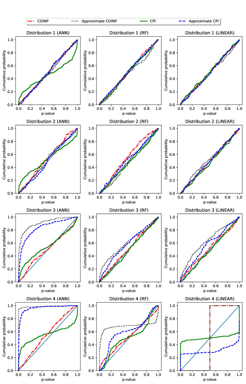
Figure 2: Cumulative distribution function of the p-values for the setting with $n=1,000$ under the null hypothesis (i.e., for choice the $\beta_{S}=0$).

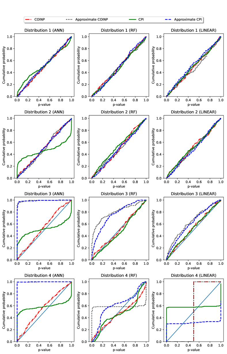
Figure 3: Cumulative distribution function of the p-values for the setting with $n=10,000$ under the null hypothesis (i.e., for choice the $\beta_{S}=0$).

Next, we compare the power function of the testing methods. Because only COINP and CPI had valid p-values, we restrict the comparisons to these methods. Figures 4 and 5 show the power of each test as a function of $\beta_{S}$. The plot indicates that all procedures achieve higher power as $\beta_{S}$ increases. Moreover, in most settings COINP leads to better power than CPI. In these examples, higher power is achieved when using a linear regression for COINP. This can be explain by the fact that in all settings the true nature of the conditional distribution of $Y|{\mathbf{x}}$ is close to linear. By comparing the COINP results from Figures 4 and 5, it is also clear the for larger sample sizes (Figure 5), the power of COINP is larger. This indicates that the testing procedure is consistent.

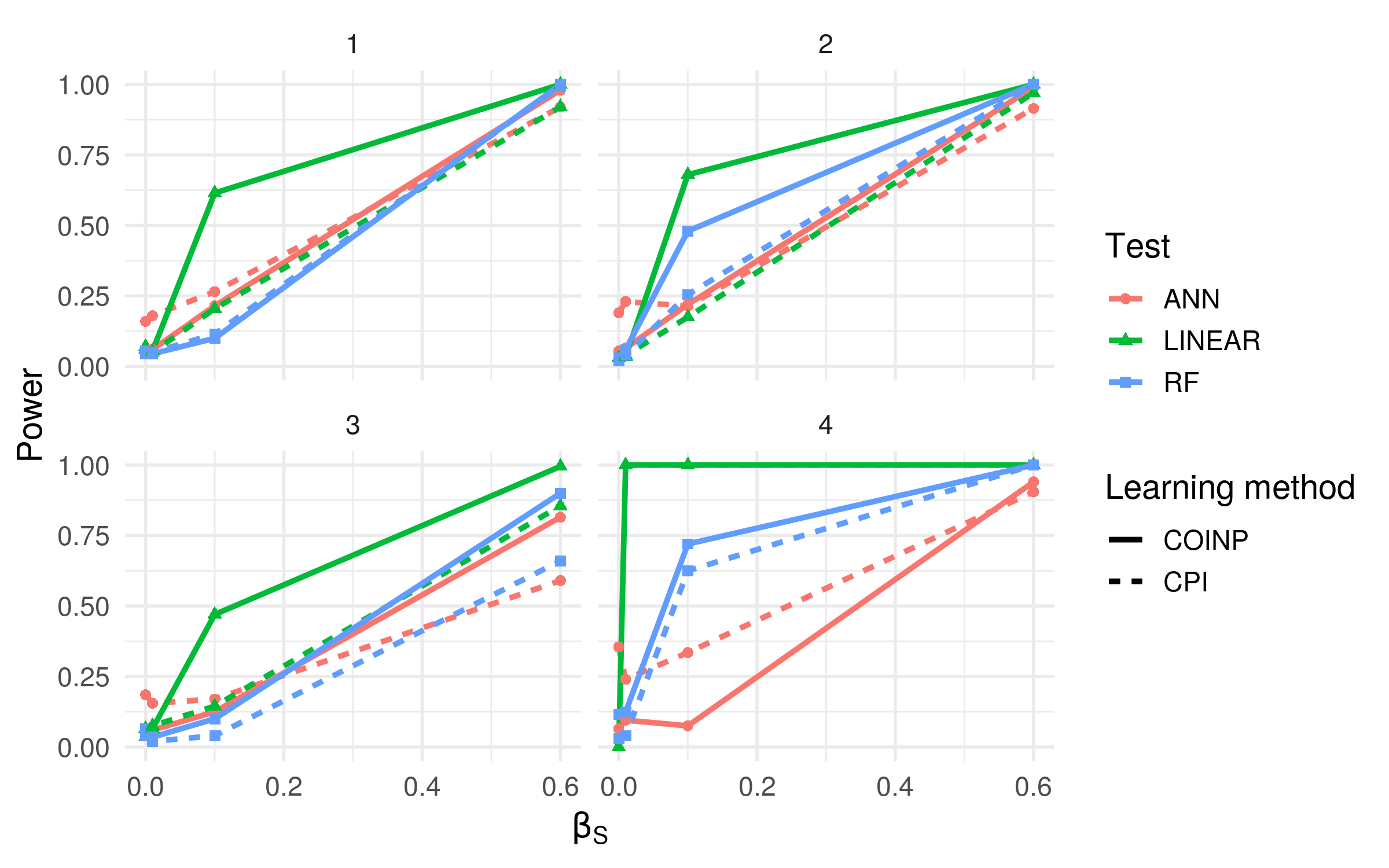
Figure 4: Power function for all setting with $n=1,000$ for $\alpha=5\%$.

Figure 5: Power function for all setting with $n=10,000$ for $\alpha=5\%$.

4 A dataset analysis example

As an illustrative example, we take the classical diamonds dataset which is readily available from ggplot2 library and Kaggle. We work with price as the response variable.

In Table 2, we present the p-values for each model together with the classical importance measure obtained from random forests.

Table 2: P-values for hypothesis testing for each comparison method compared to Random forest traditional importance measures.

		carat	depth	table	x	y	z	cut	color	clarity
ann	App COINP	0.00	0.00	0.00	0.00	0.00	0.00	0.00	0.00	0.00
	App CPI	0.00	0.02	0.03	0.00	0.00	0.00	0.00	0.00	0.00
	COINP	0.00	0.60	0.99	0.06	0.38	0.78	0.01	0.00	0.00
	CPI	0.01	1.00	0.00	0.00	1.00	0.89	0.17	0.00	0.00
linear	App COINP	0.00	0.00	0.00	0.00	0.33	0.89	0.00	0.00	0.00
	App CPI	0.00	0.02	0.00	0.00	0.06	0.01	0.00	0.00	0.00
	COINP	0.00	0.00	0.00	0.00	0.27	0.92	0.00	0.00	0.00
	CPI	0.00	0.02	0.07	0.00	0.00	0.01	0.03	0.00	0.00
rf	App COINP	0.00	0.00	0.00	0.00	0.00	0.00	0.00	0.00	0.00
	App CPI	0.00	0.00	0.04	0.00	0.00	0.00	0.00	0.00	0.00
	COINP	0.00	0.05	0.00	0.04	0.00	0.02	0.00	0.00	0.00
	CPI	0.00	0.38	0.03	0.17	0.00	0.19	0.34	0.00	0.00
RF Imp measure		0.60	0.01	0.00	0.01	0.28	0.01	0.00	0.03	0.06

5 Final remarks

We have developed a novel approach for testing conditional independence under a predictive setting. We have shown that the p-values obtained by our approach are proper, and that our hypothesis test has larger power than competing approaches under a variety of settings.

When compared to CPI, our approach is especially appealing for small sample sizes, because (i) it does not rely on asymptotic approximations such as those required by the t-test, and (ii) its computational burden is not high in those cases.

Acknowledgments

Marco Henrique de Almeida Inacio is grateful for the financial support of CAPES: this study was financed in part by the Coordenação de Aperfeiçoamento de Pessoal de Nível Superior - Brasil (CAPES) - Finance Code 001. Rafael Izbicki is grateful for the financial support of FAPESP (2017/03363-8) and CNPq (306943/2017-4).

References

- (1) Thomas B. Berrett, Yi Wang, Rina Foygel Barber and Richard J. Samworth “The conditional permutation test”, 2018 eprint: arXiv:1807.05405
- (2) L. Breiman and A. Cutler “Random Forests for scientific discovery”, 2008 URL: https://www.stat.berkeley.edu/~breiman/RandomForests/ENAR_files/frame.htm
- (3) Leo Breiman “Random forests” In Machine learning 45.1 Springer, 2001, pp. 5–32
- (4) Luis M de Campos “A scoring function for learning Bayesian networks based on mutual information and conditional independence tests” In Journal of Machine Learning Research 7.Oct, 2006, pp. 2149–2187
- (5) Krzysztof Chalupka, Pietro Perona and Frederick Eberhardt “Fast Conditional Independence Test for Vector Variables with Large Sample Sizes” In arXiv preprint arXiv:1804.02747, 2018
- (6) Djork-Arné Clevert, Thomas Unterthiner and Sepp Hochreiter “Fast and Accurate Deep Network Learning by Exponential Linear Units (ELUs)”, 2015 eprint: arXiv:1511.07289
- (7) Cees Diks and Valentyn Panchenko “A new statistic and practical guidelines for nonparametric Granger causality testing” Computing in economics and finance In Journal of Economic Dynamics and Control 30.9, 2006, pp. 1647–1669 DOI: https://doi.org/10.1016/j.jedc.2005.08.008
- (8) G Doran, Krikamol Muandet, K Zhang and B Schölkopf “A permutation-based kernel conditional independence test” In Uncertainty in Artificial Intelligence - Proceedings of the 30th Conference, UAI 2014, 2014, pp. 132–141
- (9) Aaron Fisher, Cynthia Rudin and Francesca Dominici “All Models are Wrong but many are Useful: Variable Importance for Black-Box, Proprietary, or Misspecified Prediction Models, using Model Class Reliance” In arXiv preprint arXiv:1801.01489, 2018
- (10) Xavier Glorot and Yoshua Bengio “Understanding the difficulty of training deep feedforward neural networks” In Journal of Machine Learning Research - Proceedings Track 9, 2010, pp. 249–256
- (11) Phillip Good “Permutation tests: a practical guide to resampling methods for testing hypotheses” Springer Science & Business Media, 2013
- (12) Geoffrey E. Hinton et al. “Improving neural networks by preventing co-adaptation of feature detectors” In CoRR, 2012
- (13) Sergey Ioffe and Christian Szegedy “Batch Normalization: Accelerating Deep Network Training by Reducing Internal Covariate Shift” In Proceedings of the 32nd International Conference on Machine Learning 37, Proceedings of Machine Learning Research Lille, France: PMLR, 2015, pp. 448–456 URL: http://proceedings.mlr.press/v37/ioffe15.html
- (14) Finn V Jensen “An introduction to Bayesian networks” UCL press London, 1996
- (15) Diederik P. Kingma and Jimmy Ba “Adam: A Method for Stochastic Optimization.” In CoRR abs/1412.6980, 2014
- (16) Daphne Koller and Mehran Sahami “Toward optimal feature selection” In Proceedings of the Thirteenth International Conference on International Conference on Machine Learning, 1996, pp. 284–292 Morgan Kaufmann Publishers Inc.
- (17) Judea Pearl “Causality” Cambridge university press, 2009
- (18) F. Pedregosa et al. “Scikit-learn: Machine Learning in Python” In Journal of Machine Learning Research 12, 2011, pp. 2825–2830
- (19) Rajat Sen et al. “Model-Powered Conditional Independence Test” In Advances in Neural Information Processing Systems 30 Curran Associates, Inc., 2017, pp. 2951–2961 URL: http://papers.nips.cc/paper/6888-model-powered-conditional-independence-test.pdf
- (20) Rajen D. Shah and Jonas Peters “The Hardness of Conditional Independence Testing and the Generalised Covariance Measure”, 2018 eprint: arXiv:1804.07203
- (21) Peter Spirtes et al. “Causation, prediction, and search” MIT press, 2000
- (22) Carolin Strobl et al. “Conditional variable importance for random forests” In BMC bioinformatics 9.1 BioMed Central, 2008, pp. 307
- (23) David S Watson and Marvin N Wright “Testing Conditional Predictive Independence in Supervised Learning Algorithms” In arXiv preprint arXiv:1901.09917, 2019