Exact quantum search based on analytical multiphase matching for known number of target items and the experimental demonstration on IBM Q

Abstract

In [Phys. Rev. Lett. 113, 210501 (2014)], to achieve the optimal fixed-point quantum search in the case of unknown fraction (denoted by $\lambda$) of target items, the analytical multiphase matching (AMPM) condition has been proposed. In this paper, we find out that the AMPM condition can also be used to design the exact quantum search algorithm in the case of known $\lambda$, and the minimum number of iterations reaches the optimal level of existing exact algorithms. Experiments are performed to demonstrate the proposed algorithm on IBM’s quantum computer. In addition, we theoretically find two coincidental phases with equal absolute value in our algorithm based on the AMPM condition and that algorithm based on single-phase matching. Our work confirms the practicability of the AMPM condition in the case of known $\lambda$, and is helpful to understand the mechanism of this condition.

1 Introduction

Grover quantum search algorithm [1, 2] is one of the great quantum algorithms, which achieves a quadratic speedup over classical search algorithms. Many generalizations and variants of Grover’s algorithm have been studied [3, 4, 5, 6, 7, 8, 9, 10, 11, 12, 13], especially the multiphase matching methods.

In 2008, Toyama et al. found the original multiphase matching condition [14] by means of numerical fitting, i.e.,

$$\phi_{j}=\varphi_{l+1-j},$$ (1)

to achieve success probability close to 100% over a wide range of $\lambda$ through a small number of iterations $\prod_{j=1}^{l}G\left(\phi_{j},\varphi_{j}\right)$, where $G$ is the generalized Grover operation defined by Eq. (5). However, the whole range of $\lambda\in(0,1)$ cannot be covered [14, 15].

Fortunately, in 2014, Yoder et al. proposed the analytical multiphase matching (AMPM) condition [16] which gives the analytical forms of phases $\left\{\phi_{j},\varphi_{j}\right\}$ (see Eq. (9) for details), and obtained an algorithm which can always maintain a success probability no less than $1-\delta^{2}$ on the range of $\lambda\in\left[\lambda_{0},1\right)$, where $\delta\in\left(0,1\right]$ and $\lambda_{0}$ is an arbitrary lower bound of $\lambda$. This algorithm also possesses the fixed-point property and achieves a quadratic speedup over the original fixed-point quantum search algorithm [8], showing the great fascination of the AMPM condition.

However, Ref. [16] only aims to deal with the case of unknown $\lambda$. Then, in the case of known $\lambda$, what kind of performance will the AMPM condition have? In this paper, we expect to design a quantum search algorithm with 100% success probability for the known $\lambda$ based on the AMPM condition and implement a proof-of-principle experiment, to reveal more applications of this condition.

The paper is organized as follows. Section 2 describes our analytical matched-multiphase quantum search algorithm with 100% success probability. Section 3 introduces the experimental implementation of the proposed algorithm on IBM’s cloud quantum computing platform. Section 4 discusses the connection between the AMPM condition and the single-phase matching condition, followed by a brief conclusion in Section 5.

2 Exact quantum search based on the analytical multiphase matching condition

In order to characterize the performance of the AMPM condition [16] in case of known $\lambda$, we expect to design a quantum search algorithm with 100% success probability. The specific steps are described as follows (the corresponding flow diagram is shown in Fig. 1).

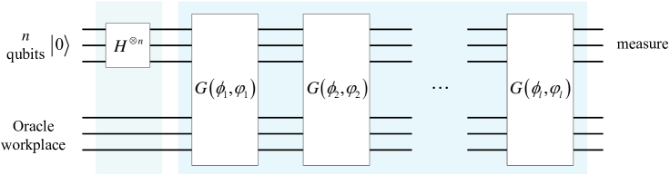
Figure 1: (Color online.) Schematic circuit for the exact matched-multiphase quantum search algorithm.

Step 1: Prepare the initial state $\left|\psi\right\rangle=H^{\otimes n}\left|0\right\rangle$, which can be written as

$$\left|\psi\right\rangle=\sqrt{\lambda}\left|\alpha\right\rangle+\sqrt{1-\lambda}\left|\beta\right\rangle,$$ (2)

where $H$ is the Hadamard transform, $\left|\alpha\right\rangle$ ($\left|\beta\right\rangle$) is the equal superposition of all target (nontarget) states, i.e.,

$$\left|\alpha\right\rangle = \frac{1}{\sqrt{M}}\sum\limits_{x\in f^{-1}\left(1\right)}\left|x\right\rangle,$$ (3)

$$\left|\beta\right\rangle = \frac{1}{\sqrt{N-M}}\sum\limits_{x\in f^{-1}\left(0\right)}\left|x\right\rangle,$$ (4)

and $\lambda=M/N$, $M$ is the number of target items in the database of size $N$.

Step 2: Perform on $\left|\psi\right\rangle$ the sequence of matched-multiphase Grover operations $\prod_{j=1}^{l}G\left(\phi_{j},\varphi_{j}\right)$, where $G\left(\phi,\varphi\right)$ is the Grover iteration with arbitrary phases, i.e.,

$$G\left(\phi,\varphi\right) = -HS_{0}^{\phi}HS_{f}^{\varphi},$$ (5)

$S_{f}^{\varphi}$ and $S_{0}^{\phi}$ represent the selective phase shifts,

$$S_{f}^{\varphi} = I-\left(-e^{i\varphi}+1\right)\sum_{x\in f^{-1}\left(1\right)}\left|x\right\rangle\left\langle x\right|,$$ (6)

$$S_{0}^{\phi} = I-\left(-e^{i\phi}+1\right)\left|0\right\rangle\left\langle 0\right|,$$ (7)

$l$ is the number of iterations, satisfying

$$l\geq\left\lceil\frac{\pi}{4\arcsin\sqrt{\lambda}}-\frac{1}{2}\right\rceil\equiv l_{{\rm min}},$$ (8)

and $\left\{\phi_{j},\varphi_{j}\right\}$ meet the analytical multiphase matching condition [16], i.e.,

$$\phi_{j}=\varphi_{l-j+1}=-2{\rm arccot}\left(\sqrt{1-\gamma^{2}}\tan\left(2\pi j/L\right)\right),\thinspace{\rm for}\thinspace 1\leq j\leq l,$$ (9)

where $L=2l+1$, $\gamma=T_{1/L}^{-1}\left(1/\delta\right)$, $T_{L}\left(x\right)=\cos\left[L\arccos\left(x\right)\right]$ is the $L^{{\rm th}}$ Chebyshev polynomial of the first kind [17], and

$$\delta=T_{L}^{-1}\left(\frac{\cos\left(\frac{\pi}{2L}\right)}{\sqrt{1-\lambda}}\right).$$ (10)

Step 3: Measure the system. This will produce one of the marked states with 100% success probability.

Reasons for the selection of $l$ of Eq. (8) and $\delta$ of Eq. (10) are as follows. First, according to Ref. [16], the final state of Step 2 can be written as

$$\left|C_{L}\right\rangle=\sqrt{P_{L}}\left|\alpha\right\rangle+\sqrt{1-P_{L}}\left|\beta\right\rangle,$$ (11)

where $P_{L}$ denotes the success probability,

$$P_{L}=1-\delta^{2}T_{L}^{2}\left[T_{1/L}\left(1/\delta\right)\sqrt{1-\lambda}\right],$$ (12)

Then, let $P_{L}=1$, we can obtain all the $k$ maximum points of $P_{L}$, denoted as

$$\lambda_{l,j}^{\delta,\max}=1-\gamma^{2}\cos^{2}\left(\frac{2j-1}{2L}\pi\right),\thinspace 1\leq j\leq l,$$ (13)

and

$$\min\left\{\lambda_{l,j}^{\delta,\max}:1\leq j\leq k\right\} = \lambda_{l,j=1}^{\delta,\max},$$ (14)

$$\min\left\{\lambda_{l,j=1}^{\delta,\max}:0<\delta\leq 1\right\} = \lambda_{l,j=1}^{\delta=1,\max}.$$ (15)

Note that, making the success probability at $\lambda$ reach 100% is the equivalent of having $\lambda$ happen to be a certain maximum point, and the range of maximum points $\big{\{}\lambda_{l,j}^{\delta,\max}\big{\}}$ is $\big{[}\lambda_{l,j=1}^{\delta=1,\max},1\big{)}$. Therefore, $\lambda\geq\lambda_{l,j=1}^{\delta=1,\max}$ is required, yielding the result of Eq. (8) of the number of iterations $l$. Let $\lambda=\lambda_{l,j=1}^{\delta,\max}$, we can further obtain the condition Eq. (10) of $\delta$. Finally, the phases $\left\{\phi_{j},\varphi_{j}\right\}$ can be calculated from Eq. (9).

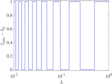
Figure 2: (Color online.) Difference between the minimum number of iterations ($l_{{\rm min}}$) of our algorithm and the optimal number of iterations ($l_{{\rm G}}$) of the original Grover algorithm as a function of the fraction $\lambda$ of target items.

At this point, all the selection methods of parameters in our exact algorithm have been obtained. Figure 2 plots the minimum number of iterations ($l_{{\rm min}}$) of our algorithm and the optimal number of iterations ($\left\lceil\frac{\pi}{4\arcsin\sqrt{\lambda}}\right\rceil-1\equiv l_{{\rm G}}$ [18]) of the original Grover algorithm as a function of $\lambda$, which shows that the difference is up to one. In fact, it can be found that our minimum number of iterations $l_{{\rm min}}$ of Eq. (8) is just the same as that of the existing exact quantum search algorithms [19, 20, 21, 22, 23], according to Eq. (7) of Ref. [19], Eqs. (15), (20) and (23) of Ref. [22], and Theorem 4 of Ref. [23].

3 Experimental implementation

We also conducted an experiment to demonstrate the proposed algorithm on the IBM’s 5-qubit computer (ibmqx4) [24].

As shown in Fig. 1, our algorithm is mainly composed of the generalized Grover operation $G\left(\phi,\varphi\right)$, defined by Eq. (5). According to Ref. [16], a quantum circuit for realizing $G\left(\phi,\varphi\right)$ is shown in Fig. 3, where $U_{f}$ is the Oracle operator, $U_{f}\left|x\right\rangle\left|y\right\rangle=\left|x\right\rangle\left|y\oplus f\left(x\right)\right\rangle$, $H$ is the Hadamard transform, and $U_{1}\left(x\right)$ is the quantum gate defined by

$$U_{1}\left(x\right)=\left[\begin{array}[]{cc}1&0\\ 0&e^{ix}\end{array}\right].$$ (16)

Note that, for the single-qubit quantum search, $S_{0}^{\phi}$ can be implemented simply by $U_{1}\left(-\phi\right)$, up to a global phase.

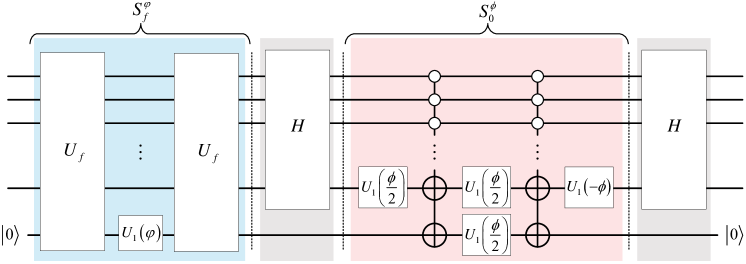
Figure 3: (Color online.) Circuit for performing the generalized Grover operation $G\left(\phi,\varphi\right)$ of Eq. (5).

For the sake of simplicity, we chose the single-qubit ($N=2$) and single-solution ($M=1$) example for experimentation. All the two possible Oracles are shown in Fig. 4.

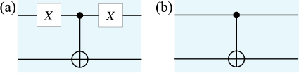
Figure 4: (Color online.) Circuits for all the possible Oracles in the single-qubit and single-solution quantum search, where (a) $f\left(0\right)=1$ and (b) $f\left(1\right)=1$.

From Eq. (8), it follows that the required number of iterations $l\geq 1$ for $\lambda=0.5$. Here, we respectively choose $l=1$, $2$ and $3$ to verify the results of the algorithm for the two possible Oracles. Corresponding parameters are shown in Table 1.

$l$	$\delta$	$\phi_{1},\phi_{2},\cdots,\phi_{l}$	$\varphi_{1},\varphi_{2},\cdots,\varphi_{l}$
1	0.272166	$\pi/2$	$\pi/2$
2	0.035103	-0.904557	2.237036
		2.237036	-0.904557
3	0.005398	-1.717287	2.501328
		0.640265	0.640265
		2.501328	-1.717287

Table 1: Parameters of our exact algorithm for $\lambda=0.5$ with $l=1$, $2$ and $3$.

As an example, the complete quantum circuit for $l=1$ with the Oracle corresponding to $f\left(1\right)=1$ is depicted in Fig. 5.

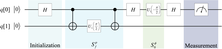
Figure 5: (Color online.) Complete circuit for one iteration of the exact analytical matched-multiphase quantum search with the Oracle corresponding to $f\left(1\right)=1$.

Figure 6 exhibits the obtained experimental results, where the white and red (grey) bars represent the theoretical and experimental probabilities, respectively.

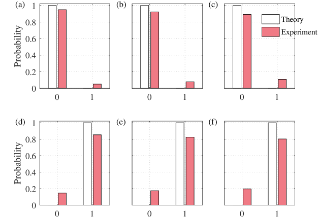
Figure 6: (Color online.) Experimental results. (a-c) and (d-f) correspond to $f\left(0\right)=1$ and $f\left(1\right)=1$, (a,d), (b,e) and (c,f) correspond to $l=1$, 2 and 3, and the white and red (grey) bars correspond to the theoretical and experimental probabilities, respectively.

Ideally, when $f\left(0\right)=1$, the output is in $\left|0\right\rangle$ with a probability of 100%, and another 0% probability yields $\left|1\right\rangle$. When $f\left(1\right)=1$, probabilities are just the opposite. To characterize the overlap between experimental and theoretical results, we adopt the statistical fidelity [25, 26]

$$F=\sum_{j=0}^{1}\sqrt{p_{j}^{{\rm exp}}p_{j}^{{\rm th}}},$$ (17)

where $p_{j}^{{\rm th}}$ and $p_{j}^{{\rm exp}}$ represent the theoretical and experimental output probabilities of the state $\left|j\right\rangle$, respectively. According to the data in Fig. 6 (a-f), the fidelities can be calculated as 0.9743, 0.9601, 0.9443, 0.9242, 0.9089 and 0.8966, which confirms the feasibility of our algorithm. The deviations between experimental and theoretical results are mainly related to errors in the readout and quantum gates. Calibration data provided by the IBM platform shows that readout error is $3.60\times 10^{-2}$ and gate error is $1.12\times 10^{-3}$.

4 Discussions

Although the AMPM condition [16] differs significantly from the single-phase matching condition [27, 28, 29, 30], we find out a coincidental connection between them. The specific discussions are as follows.

In the exact quantum search algorithm [19] based on the single-phase matching condition [27], the sequence of operations is given by $G^{l}(\phi,\varphi)$, where $\phi$ and $\varphi$ meet the condition

$$\phi=\varphi,$$ (18)

and the value of phase $\phi$ is given by

$$\pm\arccos\left(1-\frac{1-\cos\left(\frac{\pi}{2l+1}\right)}{\lambda}\right)\equiv\phi_{{\rm s}}.$$ (19)

When $\lambda=1/2$, $\phi_{{\rm s}}=\pm\frac{\pi}{2}$, $\pm 0.904557$ and $\pm 0.640265$ for $l=1$, 2 and 3. Compared with Table 1, we can see that in the case of same number of iterations, it seems that there is always a phase in the exact analytical multiphase matching quantum search algorithm, of which the absolute value is exactly the same as that of phase $\phi_{{\rm s}}$ in the exact single-phase matching algorithm.

In fact, we can prove that there indeed exists a phase $\phi_{m}$ in $\left\{\phi_{j}:1\leq j\leq l\right\}$, satisfying

$$\phi_{m}=\begin{cases}\left|\phi_{{\rm s}}\right|,&{\rm if}\thinspace l\thinspace{\rm is\thinspace odd,}\\ -\left|\phi_{{\rm s}}\right|,&{\rm if}\thinspace l\thinspace{\rm is\thinspace even,}\end{cases}$$ (20)

where

$$m=\begin{cases}\left(l+1\right)/2,&{\rm if}\thinspace l\thinspace{\rm is\thinspace odd,}\\ l/2,&{\rm if}\thinspace l\thinspace{\rm is\thinspace even.}\end{cases}$$ (21)

Reasons are as follows. On the one hand, from Eq. (19) it follows that

$$\frac{\cot^{2}\left(\frac{\phi_{{\rm s}}}{2}\right)}{\lambda-\sin^{2}\left(\frac{\pi}{2L}\right)}=\frac{1}{\sin^{2}\left(\frac{\pi}{2L}\right)}.$$ (22)

On the other hand, from Eq. (9), we have

$$\phi_{m}=-2{\rm arccot}\left(\sqrt{1-\gamma^{2}}\tan\left(2\pi m/L\right)\right),$$ (23)

where $\gamma=T_{1/L}^{-1}\left(1/\delta\right)$, $L=2l+1$, and $\delta$ meets the condition of Eq. (10). Then, substitute $\delta$ and $\gamma$ into Eq. (23), we obtain

$$\frac{\cot^{2}\left(\frac{\phi_{m}}{2}\right)}{\lambda-\sin^{2}\left(\frac{\pi}{2L}\right)}=\frac{\tan^{2}\left(\frac{2m\pi}{L}\right)}{\cos^{2}\left(\frac{\pi}{2L}\right)}.$$ (24)

Note that, according to Eq. (21), $4m\pi=\left(L\pm 1\right)\pi$, then we have

$$\tan^{2}\left(\frac{4m\pi}{2L}\right)=\cot^{2}\left(\frac{\pi}{2L}\right).$$ (25)

Therefore, based on Eqs. (22), (24) and (25), we can see that

$$\left|\phi_{m}\right|=\left|\phi_{{\rm s}}\right|.$$ (26)

Finally, due to $\phi_{\frac{l+1}{2}}>0$ and $\phi_{\frac{l}{2}}<0$, Eq. (20) holds.

5 Conclusion

In summary, we have studied the new application of the analytical multiphase matching (AMPM) condition specially for the case of known $\lambda$, i.e., based on the AMPM condition, we designed a quantum search algorithm with 100% success probability for any given $\lambda\in(0,1)$. We derived all maximum points (value of 100%) of the success probability after applying the analytical matched-multiphase Grover operations $l$ times, and further obtained the available number of iterations, phases, and other parameters, which ensure $\lambda$ just fall at a certain maximum point. Moreover, as an example, we experimentally verified the single-qubit and single-solution algorithm for all possible Oracles. Experimental results agree well with the theoretical expectations, confirming the feasibility of the proposed algorithm. The number of iterations of our algorithm is up to 1 more than the original Grover algorithm, and achieves the optimal level of the existing exact quantum search algorithms. In addition, we theoretically proved that in our exact algorithm based on the AMPM condition there coincidentally exists a phase of which the absolute value is exactly equal to that of the phase in the exact algorithm based on the single-phase matching condition. Our study confirms the usefulness of the AMPM condition in the case of known $\lambda$, and also provides a guideline to understand the mechanism and expand more applications of this condition.

References

References

- [1] L. K. Grover, A fast quantum mechanical algorithm for database search, in: Proceedings of the Twenty-eighth Annual ACM Symposium on Theory of Computing, ACM, New York, 1996, pp. 212–219.
- [2] L. K. Grover, Quantum mechanics helps in searching for a needle in a haystack, Phys. Rev. Lett. 79 (2) (1997) 325–328.
- [3] L. K. Grover, Quantum computers can search rapidly by using almost any transformation, Phys. Rev. Lett. 80 (1998) 4329–4332.
- [4] M. Boyer, G. Brassard, P. Høyer, A. Tapp, Tight bounds on quantum searching, Fortschr. Phys. 46 (4-5) (1998) 493–505.
- [5] D. Biron, O. Biham, E. Biham, M. Grassl, D. A. Lidar, Generalized Grover search algorithm for arbitrary initial amplitude distribution, in: C. P. Williams (Ed.), Quantum Computing and Quantum Communications, Springer, Berlin, 1999, pp. 140–147.
- [6] P. Høyer, Arbitrary phases in quantum amplitude amplification, Phys. Rev. A 62 (2000) 052304.
- [7] A. Younes, J. Rowe, J. Miller, Quantum search algorithm with more reliable behaviour using partial diffusion, AIP Conf. Proc. 734 (1) (2004) 171–174.
- [8] L. K. Grover, Fixed-point quantum search, Phys. Rev. Lett. 95 (15) (2005) 150501.
- [9] T. Li, W.-S. Bao, W.-Q. Lin, H. Zhang, X.-Q. Fu, Quantum search algorithm based on multi-phase, Chin. Phys. Lett. 31 (5) (2014) 050301.
- [10] A. M. Dalzell, T. J. Yoder, I. L. Chuang, Fixed-point adiabatic quantum search, Phys. Rev. A 95 (1) (2017) 012311.
- [11] T. Byrnes, G. Forster, L. Tessler, Generalized Grover’s algorithm for multiple phase inversion states, Phys. Rev. Lett. 120 (2018) 060501.
- [12] T. Li, W.-S. Bao, H.-L. Huang, F.-G. Li, X.-Q. Fu, S. Zhang, C. Guo, Y.-T. Du, X. Wang, J. Lin, Complementary-multiphase quantum search for all numbers of target items, Phys. Rev. A 98 (6) (2018) 062308.
- [13] F. Toyama, W. van Dijk, Additive composition formulation of the iterative grover algorithm, Can. J. Phys. 97 (7) (2019) 777–785.
- [14] F. M. Toyama, W. van Dijk, Y. Nogami, M. Tabuchi, Y. Kimura, Multiphase matching in the Grover algorithm, Phys. Rev. A 77 (4) (2008) 042324.
- [15] F. M. Toyama, S. Kasai, W. van Dijk, Y. Nogami, Matched-multiphase Grover algorithm for a small number of marked states, Phys. Rev. A 79 (1) (2009) 014301.
- [16] T. J. Yoder, G. H. Low, I. L. Chuang, Fixed-point quantum search with an optimal number of queries, Phys. Rev. Lett. 113 (21) (2014) 210501.
- [17] J. C. Mason, D. C. Handscomb, Chebyshev polynomials, CRC Press, Boca Raton, 2002.
- [18] M. A. Nielson, I. L. Chuang, Quantum computation and quantum information, Cambridge University Press, Cambridge, 2000.
- [19] G. L. Long, Grover algorithm with zero theoretical failure rate, Phys. Rev. A 64 (2) (2001) 022307.
- [20] F. M. Toyama, W. van Dijk, Y. Nogami, Quantum search with certainty based on modified Grover algorithms: optimum choice of parameters, Quantum Inf. Process. 12 (5) (2013) 1897–1914.
- [21] C. R. Hu, Family of sure-success quantum algorithms for solving a generalized Grover search problem, Phys. Rev. A 66 (4) (2002) 042301.
- [22] J. Y. Hsieh, C. M. Li, J. S. Lin, D. S. Chuu, Formulation of a family of sure-success quantum search algorithms, Int. J. Quantum Inf. 2 (3) (2004) 285–293.
- [23] G. Brassard, P. Høyer, M. Mosca, A. Tapp, Quantum amplitude amplification and estimation, in: S. J. Lomonaco, Jr., H. E. Brandt (Eds.), Quantum Computation and Information, American Mathematical Society, Providence, 2002, pp. 53–74.
- [24] IBM Q Experience. https://quantum-computing.ibm.com. Accessed: 1 July 2019.
- [25] H.-L. Huang, Y.-W. Zhao, T. Li, F.-G. Li, Y.-T. Du, X.-Q. Fu, S. Zhang, X. Wang, W.-S. Bao, Homomorphic encryption experiments on IBM’s cloud quantum computing platform, Front. Phys. 12 (1) (2017) 120305.
- [26] H.-L. Huang, A. K. Goswami, W.-S. Bao, P. K. Panigrahi, Demonstration of essentiality of entanglement in a Deutsch-like quantum algorithm, Sci. China Phys. Mech. 61 (6) (2018) 060311.
- [27] G. L. Long, Y. S. Li, W. L. Zhang, L. Niu, Phase matching in quantum searching, Phys. Lett. A 262 (1) (1999) 27–34.
- [28] G. L. Long, C. C. Tu, Y. S. Li, W. L. Zhang, H. Y. Yan, An SO (3) picture for quantum searching, J. Phys. A 34 (4) (2001) 861.
- [29] G.-L. Long, X. Li, Y. Sun, Phase matching condition for quantum search with a generalized initial state, Phys. Lett. A 294 (3) (2002) 143–152.
- [30] C.-M. Li, C.-C. Hwang, J.-Y. Hsieh, K.-S. Wang, General phase-matching condition for a quantum searching algorithm, Phys. Rev. A 65 (3) (2002) 034305.