Featuring the topology with the unsupervised machine learning

Abstract

Images of line drawings are generally composed of primitive elements. One of the most fundamental elements to characterize images is the topology; line segments belong to a category different from closed circles, and closed circles with different winding degrees are nonequivalent. We investigate images with nontrivial winding using the unsupervised machine learning. We build an autoencoder model with a combination of convolutional and fully connected neural networks. We confirm that compressed data filtered from the trained model retain more than $90\%$ of correct information on the topology, evidencing that image clustering from the unsupervised learning features the topology.

I Introduction

Brains ingeniously function with networks of neurons. For understanding of intrinsic brain dynamics, physicists would favorably decompose such an integral system into irreducible elements, so that we can analyze relatively simpler function of each building element that takes rather primitive actions. Then, numerical simulations on computer are handy devices to test if a postulated mechanism of brains should go as expected. Such modeling embodies non-equilibrium processes of brains, which is an approach acknowledged commonly as computational neuroscience. Besides, a hypothesis called quantum brain dynamics implements quantum fluctuations and Nambu-Goldstone bosons for brain sciences Ricciardi and Umezawa (1967); Jibu and Yasue (1995) (for discussions for/against quantum phenomena in brain dynamics, see Ref. Jedlicka (2017)), which bridges a devide between computational neuroscience and modern physics.

In contrast to such “off-equilibrium” problems, in the language of physics, perception and recognition are “static” problems. For the latter problems, model-independent research tools are available for computer simulations. That is, the machine learning enables us to emulate the neural structure of brains on computer. One of intriguing attributes of the machine learning, particularly with deep neural networks (NNs), is that any nonlinear mapping can be represented by data transmission through multiple hidden layers LeCun et al. (2015).

These days we have witnessed tremendous progresses in the field of image recognition and classification by means of the machine learning. In particular the progress has been driven by Convolutional Neural Network (CNN) LeCun et al. (1989), which was originally proposed as a multi-layer neural network imitating animal’s visual cortex Fukushima (1980). The CNN has become the most common approach for high-level image recognition since an overwhelming victory of AlexNet Krizhevsky et al. (2012) at “ImageNet Large Scale Visual Recognition Challenge 2012.” Challenges of minimizing inter-class variability, reducing error rate, achieving large-scale image recognition, etc are ongoing improvements and they are all crucial steps for practical usages.

Physicswise, the image handling with the deep learning has proved its strength in identifying phase transitions. Some successful attempts are found in Ref. Ohtsuki and Ohtsuki (2016) for two-dimensional systems analyzed by the supervised learning, Ref. Ohtsuki and Ohtsuki (2017) for its extension to three-dimensional systems, and Ref. Funai and Giataganas (2018) for statistical systems studied by the unsupervised learning. Here, we point out an essential difference between the supervised and unsupervised learning; the former is useful for regression and grouping problems, while the latter efficiently makes feature extraction and clustering of data. Interestingly, similarity between the unsupervised learning and the renormalization group in physics has also been investigated, see Ref. Iso et al. (2018).

In the context of image recognition, at the same time, a distinct direction toward more fundamental research would be as important to demystify blackboxed artificial intelligence, which may be somehow beneficial for so-called explainable artificial intelligence Samek et al. (2017); Došilović et al. (2018). The fundamental question of our interest in the present work is what would be the simplest element of images that categorizes those images into representative clusters. For the sake of image clustering, a useful mathematical notion, which underlies modern physics, has been developed known as the “topology” theorized into the form of homotopy. The most well-known example is that a mug with one handle and a torus-shaped donut belong to the same grouping class; the shape can be smoothly deformed from one to the other, and they are of the same homotopy type. In this work we report leading-edge results from our simulations with the CNN supporting an idea that the topology is critical information for image feature extraction and clustering.

II Topology and the winding number

The topology is classified by the homotopy group in mathematics. The simplest example is what is called the fundamental homotopy group denoted as $\pi_{1}(S^{1})=\mathbb{Z}$ associated with a mapping from $S^{1}$ (i.e., one dimensional unit sphere) to another $S^{1}$ and an integer $n_{W}\in\mathbb{Z}$ corresponds to the winding number. To demonstrate the idea concretely, let us consider the following function on $S^{1}$ of U(1),

$$\phi(x)=\mathrm{e}^{\mathrm{i}\theta(x)}=\cos\theta(x)+\mathrm{i}\sin\theta(x)\,.$$ (1)

If $x$ is a coordinate on a circle with period $L$, the above function represents a mapping from $S^{1}$ in coordinate space to $S^{1}$ on Gauss’ plane with Euler’s angle $\theta$ (which is also called the “lift” in homotopy theory). While $x$ travels around from 0 to $L$ under a condition, $\phi(0)=\phi(L)$, Euler’s angle $\theta$ should return to the original position modulo $2\pi$. The winding number associated with the above function (or the “degree” of this function) reads,

$$n_{W}=\frac{\theta(L)-\theta(0)}{2\pi}=\frac{\ln[\phi(L)/\phi(0)]}{2\pi\mathrm{i}}=\frac{1}{2\pi\mathrm{i}}\int_{0}^{L}\mathrm{d}x\,\phi^{-1}(x)\frac{\mathrm{d}\phi(x)}{\mathrm{d}x}\,.$$ (2)

Figure 1 schematically illustrates one winding configuration of $\phi(x)$ having $n_{W}=1$.

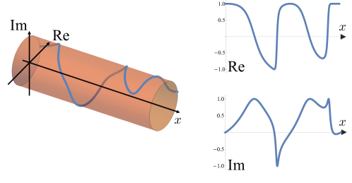
Figure 1: Schematic illustration of $\pi_{1}(S^{1})$ realized by $\phi(x)=\mathrm{e}^{\mathrm{i}\theta(x)}$. In the left representation the behavior of $\theta(x)$ is manifest and $n_{W}=1$ is easily concluded, but in our simulation, only $(\mathrm{Re\,}\phi,\mathrm{Im\,}\phi)$ as shown in the right is given to the NN model.

For us, human-beings, it would be an elementary-class exercise to discover a counting rule of $n_{W}$. If we were given many different images with correct answers of $n_{W}$, it would be just a matter of time for us to eventually find a right counting rule out. This description is nothing but the machinery of the supervised learning. Interestingly, it has been reported that the deep neural network trained by the supervised learning correctly reproduced $n_{W}$ of $\pi_{1}(S^{1})$ Zhang et al. (2018). There, the machine discovered a nice fit of the formula (2) only from the information of given $(\mathrm{Re\,}\phi,\mathrm{Im\,}\phi)$ and $n_{W}$, but not referring to $\theta(x)$ directly. In the present work, we are taking one step forward; we would like to see the NN model not only optimizing a fit from the supervised learning but featuring the topology from the unsupervised learning.

More specifically, we would like to think of classification of many images without giving the answers of $n_{W}$. It would be very intriguing to ask such a question of how the CNN makes clustering of differently winding data, which would be a prototype model of how our brains categorize images based on the topological characterization. Thus, the unsupervised learning as adopted in this work should tell us surpassing information than the supervised learning for the purpose to dissect the topological contents.

III Results and Discussions

In the numerical procedure we represent $\phi(x)$ by a sequence of numbers on discretized $x$ with $L=128$ grids, i.e., we generate $2\times 128=256$ sized data of $(\mathrm{Re\,}\phi_{i},\mathrm{Im\,}\phi_{i})$ with $i=1,\dots,L$ under the periodic boundary condition; $(\mathrm{Re\,}\phi_{L},\mathrm{Im\,}\phi_{L})=(\mathrm{Re\,}\phi_{1},\mathrm{Im\,}\phi_{1})$. These 256 numbers consist of the input data onto the CNN side.

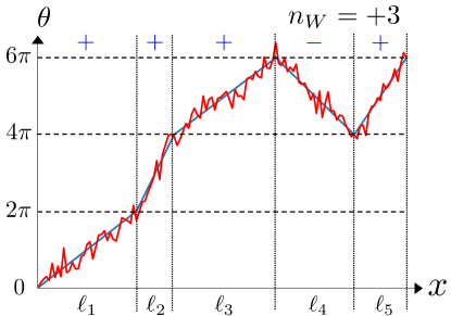
Figure 2: One example of generated data for $(+,+,+,-,+)$ with $n_{W}=+3$.

We prepare the training and test data randomly. We will give more detailed explanations on the numerical procedure in Method. Each data consists of distinct $N_{s}$ segments along $x$ with either positive or negative winding, where the segment lengths, $\ell_{m}$, are chosen randomly, where $\displaystyle\sum_{m=1}^{N_{s}}\ell_{m}=L$ should be kept. For the data used in this work, we take account of $N_{s}=0,1,2,3,4$, and $5$. We then assign positive and negative winding randomly to each segment, which is symbolically labeled as $(p_{1},p_{2},\dots,p_{N_{s}})$ with $p_{m}=\pm 1$, where $+$ (and $-$) stands for positive (and negative, respectively) winding. For example, $(+,+,+,-,+)$ for $N_{s}=5$ is a configuration with net winding, $\displaystyle n_{W}=\sum_{m=1}^{N_{s}}p_{m}=+3$. In $m$-th segment we first postulate that $\theta(x)$ linearly changes its value by $2\pi p_{m}$. Then, zigzag lines are distorted with random noises to enhance the learning quality and thus the adaptivity. Figure 2 depicts an example of generated data with a choice of $(+,+,+,-,+)$. With $N_{s}$ up to 5 $2^{0}+2^{1}+2^{2}+2^{3}+2^{4}+2^{5}=63$ winding patterns are possible, and $n_{W}$ can take a value from $-5$ to $+5$. This setup is for the moment sufficiently general for our goal to check performance of the topology detection.

The unsupervised learning utilizes the autoencoder Hinton and Salakhutdinov (2006); it first encodes the data compressed into smaller number of neurons in the CNN (in our case, 16 sites $\times$ 4 filters from original 256 sites) and then decodes the compressed data with fully connected NN into the original size. We repeat such encoding and decoding processes to minimize the loss function measured by the squared difference between the original input data and the coarse-grained output data. The learning process optimizes the filters in the CNN encoder and simultaneously the weights in the NN decoder.

We shall see the results from our NN model that has been optimized by the unsupervised learning with the training dataset of 63 winding patterns times 1,000 randomly generated data (i.e., 63,000 data in total). We input the test data into the optimized NN model and observe feature maps of 16 neurons convoluted with 4 filters on the deepest CNN layer. Figure 3 summarizes sampled feature maps from the 1st filter. The left plot is for $N_{s}=5$ with all possible winding patterns averaged over 1,000 test data. The right plot particularly picks up the averaged feature maps for five different windings with $N_{s}=5$ and $n_{W}=+3$. At a glance one may think that the behavior looks like coarse-grained $\mathrm{Re\,}\phi(x)$ or $\mathrm{Im\,}\phi(x)$ with segment lengths normalized.

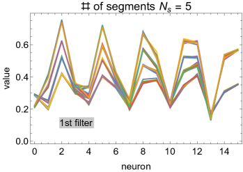
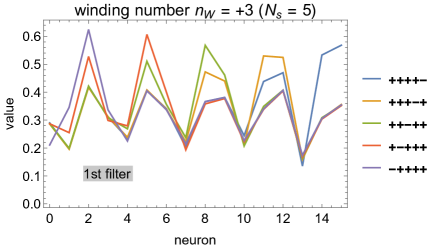
Figure 3: Examples of feature maps on the deepest CNN layer. (Left) $N_{s}=5$ and all possible (i.e., $2^{5}=32$) winding patterns averaged over 1,000 test data. (Right) $N_{s}=5$ with $n_{W}=+3$ fixed and five winding patterns averaged over 1,000 test data.

Now, the most fascinated question is whether the compressed data on 16 sites convoluted with 4 filters could retain information on the topology or not, and if yes, how we can retrieve it. From the left of Fig. 3 it is obvious that the peak heights reflect different winding patterns. In fact, the averaged feature maps exhibit a clear hierarchy of four separated heights with one-to-one correspondance to the winding sequence; that is, the peak heights increase with sequential windings as

$$(+,+)~{}~{}<~{}~{}(+,-)~{}~{}<~{}~{}(-,+)~{}~{}<~{}~{}(-,-)\,,$$ (3)

and the height at the far right end is determined solely by $\pm$, which is due to zero-padding in the convolution to keep the data size.

For example, if we see the far left peak around the 2nd neuron in the right of Fig. 3, $(-,+,+,+,+)$ has the highest peak, $(+,-,+,+,+)$ the second highest, and others are degenerated in accord with Eq. (3). Also, we notice in the right of Fig. 3 that, for $(+,+,+,+,-)$, three consecutive short peaks appear from the left, one middle peak follows, and then one tall peak sits at the right end. The short peaks correspond to $(+,+)$ of $((+,+),+,+,-)$, $(+,(+,+),+,-)$, and $(+,+,(+,+),-)$. The middle peak corresponds to $(+,+,+,(+,-))$ and the tall peak is sensitive only to $-$ of $(+,+,+,+,-)$.

One might have thought that such a clear hierarchy as in Fig. 3 is visible only after taking the average. This is indeed the case, as exemplified in Fig. 4; the feature maps for one test data do not always show prominent peaks with well separated heights. Nevertheless, surprisingly, we can see that such fluctuating coarse-grained data in Fig. 4 still retain information on the topology!

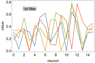
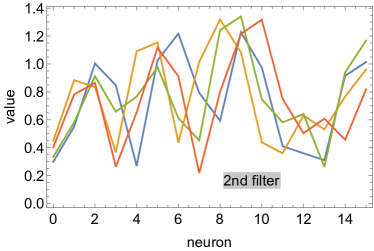
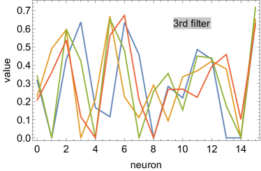
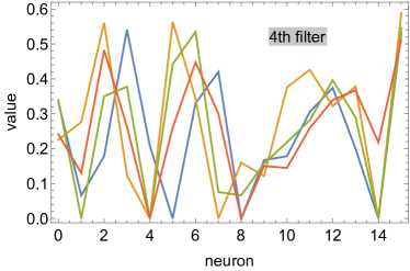
Figure 4: Feature maps from the 1st filter (top-left), the 2nd filter (top-right), the 3rd filter (bottom-left), and the 4th filter (bottom-right) for $(+,+,+,-,+)$ data without taking the average. Four randomly selected data are shown by four different colors.

It is impossible for our eyes to recognize any topological contents from Fig. 4, so we will ask for a help of another machine learning device. For each of 63,000 training data, we have such feature maps like Fig. 4 and also the corresponding $n_{W}$. We can then perform the supervised learning to train a fully connected NN (with one hidden layer) such that the output gives the probability distribution of guessed $n_{W}$ (out of $-5,\ldots,5$) in response to the input of feature maps. Figure 5 is the correct answer rate. If we input the feature maps from only 1 filter, the most-likely $n_{W}$ hits the correct value at the rate of $50\%$, and the second-likely one at the rate of $31\%$. If we use the feature maps from 2 filters, the available information is doubled, and the correct answer rate of the most-likely $n_{W}$ becomes $78\%$. Amazingly, for the feature maps from 3 filters, it increases up to $90\%$! There is almost no difference between the 3-filter and the 4-filter results, and it seems that the correct answer rate is saturated at $90\%$.

To summarize, from these results and analyses, we can conclude that the coarse-grained data of the feature maps through the unsupervised learning do retain information on the topology. In other words, the unsupervised learning with autoencoder can provide us with a nontrivial machinery to compress data without losing the topological contents.

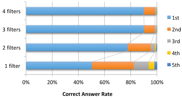
Figure 5: Correct answer rate for $n_{W}$ guessed from the feature maps. For each of 63,000 test data we have checked where the correct winding number ranks (1st, 2nd, … in the legend) in the probability output from the supervised NN model.

IV Discussion

We demonstrated that the unsupervised machine learning of images makes feature extraction without losing information on the topology. This evidences that the winding number corresponding to the fundamental group, $\pi_{1}(S^{1})$, should be one of the essential indices that characterize image clustering. We trained an autoencoder with the CNN and the fully connected NN for the unsupervised learning using randomly generated data of functions from $x$ on $S^{1}$ to a U(1) element. We found that the averaged feature maps on the deepest CNN layer show a clear hierarchy pattern of the configurations with one-to-one correspondence to the winding sequences. With help of the supervised learning technique we also revealed that feature maps for each image data look coarse-grained images and such compressed data retain information on the topology correctly.

The extension of the present work, i.e., the unsupervised learning of higher-dimensional images with nontrivial winding would be quite interesting. We note that the supervised machine learning has been utilized for $\pi_{2}(S^{2})$ Zhang et al. (2018), but as we illustrated in this work, the unsupervised machine learning would be more interesting. Implications from this extension include intriguing applications in quantum field theories. In fact, some classical solutions of the equations of motion in quantum field theory are topologically stabilized. In such cases the field configurations are classified according to the winding number. For representative examples, $\pi_{2}({\rm SU(2)/U(1)})=\mathbb{Z}$ for monopoles, $\pi_{3}({\rm SU(2)})=\mathbb{Z}$ for Skyrmions (with no time-dependence), and $\pi_{3}({\rm SU(2)})=\mathbb{Z}$ for instantons (with the fields at infinity identified) in pure Yang-Mills theory Belavin et al. (1975); ’t Hooft (1976). Actually, it is a long-standing problem how to visualize the topological contents in quantum field theories. The numerical lattice simulation is a powerful tool to solve quantum field theories, and field configurations should in principle contain information on the topology. Some algorithms to extract topologically nontrivial configurations such as monopoles, Skyrmions, and instantons have been proposed Berg (1981); Teper (1986); Ilgenfritz et al. (1986). The most well-known approach, i.e., the cooling method has a serious flaw, however. If the cooling is applied too many times, the topology is lost and the field configuration would become trivially flat. Therefore, the cooling procedures should be stopped at some point, and this artificial termination of the procedures causes uncertainties. Alternatively, we would emphasize that the compression of field configuration images by means of the unsupervised machine learning is a promising candidate for the superior smearing algorithm not to lose the topological contents. We are testing this idea in simple two-dimensional lattice model, namely, $\mathbb{C}P^{N-1}$ model that has $\pi_{2}(S^{2})$ instantons.

Mathematically, it would be also a very interesting question to consider not only the homotopy groups but also the homology $H_{n}(X)$ of a topological space $X$ defined by a coset of cycles in $n$ dimensions over boundaries of $(n+1)$-dimensional elements. For example, $H_{0}(X)$ counts the number of connected drawings of images, and $H_{1}(X)$ counts the number of loops of images, etc. This direction of research is now ongoing.

Method

Input data of winding patterns

Input data $\phi_{i}=e^{\mathrm{i}\theta_{i}}$ ($i=1,\ldots,L$), including training data and test data, are generated in the following way. Note that since the data $\phi_{i}$ are complex numbers, we actually input the combinations of their real and imaginary parts ($\mathrm{Re\,}\phi_{i},\mathrm{Im\,}\phi_{i}$).

First we impose the periodic boundary condition:

$$\mathrm{Re\,}\phi_{1}=\mathrm{Re\,}\phi_{L},\quad\mathrm{Im\,}\phi_{1}=\mathrm{Im\,}\phi_{L}.$$ (4)

Then we divide $L$ sites into $N_{s}$ segments, and length of each segment $\ell_{m}$ ($m=1,\ldots,N_{s}$) is randomly chosen as

$$\ell_{m}=\frac{L-1}{N_{s}}\left[1+0.4(\xi_{m}-\xi_{m-1})\right]$$ (5)

where $\xi_{m}$ is a random number from a uniform distribution in the open interval $(-1,1)$. This means the lengthes in all the segments satisfy $0.2\frac{L-1}{N_{s}}<\ell_{m}<1.8\frac{L-1}{N_{s}}$. We set $\xi_{0}=\xi_{N_{s}}=0$ so that the total length $L$ is kept. To be exact, the length $\ell_{m}$ should be an integer, so the right hand side is rounded to an integer.

In each segment $m$, the angle $\theta_{i}$ is composed of a linear part from 0 to $\pm 2\pi$ and a random noise:

$$\frac{\theta_{i}}{2\pi}=p_{m}\frac{i-i_{0}}{\ell_{m}}+0.1\zeta_{i}$$ (6)

where $p_{m}=\pm 1$ is the winding direction and $i_{0}=1+\sum_{m^{\prime}=1}^{m-1}\ell_{m^{\prime}}$. The random noise $\zeta_{i}$ is from a Gaussian distribution with mean 0 and variance 1.

In our experiment, we set $L=128$ and $N_{s}=0,1,\ldots,5$. Then all the combinations of winding directions $p_{m}$ have $\sum_{N_{s}=0}^{5}2^{N_{s}}=63$ patterns. For each winding pattern, we generate 1,000 $+$ 1,000 input data with the parameters $(\xi_{m},\zeta_{i})$ chosen randomly. The first 1,000 data (in total 63,000 data) is the training data, which is used for training our autoencoder and supervised NN. The other 1,000 data is the test data for analyzing the feature maps in the autoencoder (see Figs. 3 and 4) and the output from the supervised NN (see Fig. 5).

Autoencoder

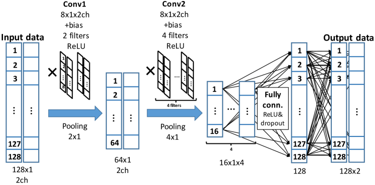
Figure 6: Schematic figure of the autoencoder used for our unsupervised learning.

The autoencoder for our unsupervised learning consists of the CNN (encoder) and the fully-connected NN (decoder). A schematic figure of our autoencoder is shown in Fig. 6. We made a training code using TensorFlow Abadi et al. (2016).

The CNN encoder has two layers. In the both layers, we use the convolution with $8\times 1(\times 2$ channel) sized filters and stride 1. We also use the zero padding to keep the size of data, and the ReLU as an activation function. In the convolution part, difference between the first and second layers is only the number of filters. After the convolution, our encoder has the pooling part in each layer. We use the max pooling with $2\times 1$ sized window and stride 2 for each channel in the first layer. This pooling compresses the data size into $1/$stride of the original size. The second layer has $4\times 1$ sized window and stride 4, then as a result, the CNN encoder outputs the feature map with $L/2/4=16$ sites (for each filter out of 4 filters), as we saw in Fig. 3.

The fully-connected NN decoder has two layers, too. In the first layer, we use the dropout method with probability 0.5 to avoid overlearning, then use the ReLU again. The final layer has no dropout and no activation function, then outputs coarse-grained data $(\varphi_{i,1},\varphi_{i,2})$ with the same size as the input data $(\mathrm{Re\,}\phi_{i},\mathrm{Im\,}\phi_{i})$.

As the loss function for the training, we choose the squared difference between input data $\phi_{i}$ and output data $\varphi_{i,j}$, that is,

$$\frac{1}{2L}\sum_{i=1}^{L}\left[(\mathrm{Re\,}\phi_{i}-\varphi_{i,1})^{2}+(\mathrm{Im\,}\phi_{i}-\varphi_{i,2})^{2}\right].$$ (7)

We prepared the training and test data, both of which contain 63 winding patterns times 1000 randomly generated data. Then we found the unsupervised learning with the learning rate $10^{-7}$ and the mini-batch size 10 decreases the loss function of the test data to its minimum around 6000 epochs, as shown in Fig. 7.

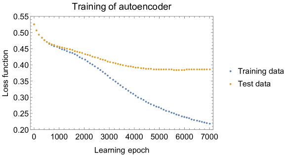
Figure 7: Loss function during training of our autoencoder.

References

- Ricciardi and Umezawa (1967) L. M. Ricciardi and H. Umezawa, Kybernetik 4, 44 (1967).
- Jibu and Yasue (1995) M. Jibu and K. Yasue, Quantum Brain Dynamics and Consciousness: An Introduction, Advances in consciousness research (J. Benjamins Publishing Company, 1995).
- Jedlicka (2017) P. Jedlicka, Frontiers in Molecular Neuroscience 10, 366 (2017).
- LeCun et al. (2015) Y. LeCun, Y. Bengio, and G. Hinton, Nature 521, 436 (2015).
- LeCun et al. (1989) Y. LeCun, B. Boser, J. S. Denker, D. Henderson, R. E. Howard, W. Hubbard, and L. D. Jackel, Neural Computation 1, 541 (1989).
- Fukushima (1980) K. Fukushima, Biological Cybernetics 36, 193 (1980).
- Krizhevsky et al. (2012) A. Krizhevsky, I. Sutskever, and G. E. Hinton, in Advances in neural information processing systems (2012) pp. 1097–1105.
- Ohtsuki and Ohtsuki (2016) T. Ohtsuki and T. Ohtsuki, Journal of the Physical Society of Japan 85, 123706 (2016).
- Ohtsuki and Ohtsuki (2017) T. Ohtsuki and T. Ohtsuki, Journal of the Physical Society of Japan 86, 044708 (2017).
- Funai and Giataganas (2018) S. S. Funai and D. Giataganas, (2018), arXiv:1810.08179 [cond-mat.stat-mech] .
- Iso et al. (2018) S. Iso, S. Shiba, and S. Yokoo, Phys. Rev. E97, 053304 (2018), arXiv:1801.07172 [hep-th] .
- Samek et al. (2017) W. Samek, T. Wiegand, and K. Müller, CoRR abs/1708.08296 (2017), arXiv:1708.08296 .
- Došilović et al. (2018) F. K. Došilović, M. Brčić, and N. Hlupić, in 2018 41st International Convention on Information and Communication Technology, Electronics and Microelectronics (MIPRO) (2018) pp. 0210–0215.
- Zhang et al. (2018) P. Zhang, H. Shen, and H. Zhai, Phys. Rev. Lett. 120, 066401 (2018).
- Hinton and Salakhutdinov (2006) G. E. Hinton and R. R. Salakhutdinov, Science 313, 504 (2006).
- Belavin et al. (1975) A. A. Belavin, A. M. Polyakov, A. S. Schwartz, and Yu. S. Tyupkin, Phys. Lett. B59, 85 (1975).
- ’t Hooft (1976) G. ’t Hooft, Phys. Rev. D14, 3432 (1976).
- Berg (1981) B. Berg, Phys. Lett. 104B, 475 (1981).
- Teper (1986) M. Teper, Phys. Lett. B171, 86 (1986).
- Ilgenfritz et al. (1986) E.-M. Ilgenfritz, M. Müller-Preuker, G. Schierholz, H. Schiller, et al., Proceedings, 23RD International Conference on High Energy Physics, JULY 16-23, 1986, Berkeley, CA, Nucl. Phys. B268, 693 (1986).
- Abadi et al. (2016) M. Abadi, P. Barham, J. Chen, Z. Chen, A. Davis, J. Dean, M. Devin, S. Ghemawat, G. Irving, M. Isard, M. Kudlur, J. Levenberg, R. Monga, S. Moore, D. G. Murray, B. Steiner, P. Tucker, V. Vasudevan, P. Warden, M. Wicke, Y. Yu, and X. Zheng, in 12th USENIX Symposium on Operating Systems Design and Implementation (OSDI 16) (USENIX Association, Savannah, GA, 2016) pp. 265–283.