Theory of surface-induced multiferroicity in magnetic materials, thin films and multilayers

Abstract

We present a theoretical study of the onset of electric polarization close to a surface in magnetic materials and in thin films and multilayers. We consider two different paths that lead to the onset of multiferroic behavior at the boundary in materials that are bulk collinear ferromagnets or antiferromagnets. These two paths are distinguished by the presence or absence of a surface induced Dzyaloshinskii-Moriya interaction which can be taken into account through Lifshitz invariants in the free energy of the system. Experimental consequences are discussed in the light of the developed theory.

I Introduction.

Magnetoelectric multiferroic materials continue to attract much interest, due to both scientific as well as technological importance Khomskii ; Wang ; lottermoser . Typically the ferroelectric transition temperature is much higher than the magnetic one and a coupling between the two order parameters is weak. Representative examples are the transition metal perovskites BiFeO₃, BiMnO₃, belonging to type I class of multiferroics (more details on the classification Khomskii ; cheong ; eerenstein ; Ramesh ; ederer ). When the two ordering temperatures are close or even coincide, such as in TbMnO₃ kimura or TbMn₂O₅ hur strong multiferroic behavior is expected. From the symmetry point of view, the necessity to break both inversion and time-reversal symmetries suggests different possible mechanisms which have been actually realised. In type II multiferroics, magnetism drives the onset of the ferroelectric order parameter, either due to the presence of spin-orbit coupling (SOC) and magnetic frustration e.g. in Ni₃V₂O₆ lawes ; mostovoy ; katsura , or exchange striction e.g. in TbMnO₃ and Ca₃CoMnO₆ sergienko ; Wu or ”phase dislocated” spin density waves e.g. in YMn₂O₅ chapon ; betouras .

Currently the role of surfaces and interfaces in the properties of materials is the focus of systematic studies Panagopoulos1 ; Gerhard ; Maruyama ; Zutic ; Hu . In technological applications there are important prospects and the theoretical understanding is developing Hellman ; Sander . Experimental techniques have been advanced such that novel phenomena can be detected as a result of the higher precision and resolution. Recent advancements led to the detection of new properties, by distinguishing surface from bulk phenomena or going to the atomic scale UO2 ; Sonntag .

In this work, we study the effects of boundaries in the development of multiferroic behavior in bulk materials, thin films and multilayers. This is a complementary effort to first-principles calculations on the magnetoelectric coupling close to surfaces Tsymbal or monolayers Nakamura of specific materials. A straightforward Ginzburg-Landau (GL) free-energy analysis with appropriate boundary conditions demonstrates that collinear magnetism can generate a ferroelectric polarization near surfaces, even without invoking the mechanism of phase dislocation betouras . In addition, due to the absence of inversion symmetry close to surfaces, a term that promotes the Dzyaloshinskii-Moriya interaction (DMI) can be present, leading to multiferroic behaviour through the formation of spiral magnetic order mostovoy ; katsura . The underlying assumption is that we deal with predominantly magnetic materials with non-zero coupling between magnetic and ferroelectric order parameters. In the following, we analyse separately the two mechanisms.

II Ginzburg-Landau analysis.

We focus on a simple cubic ferromagnet, for simplicity, without frustration. Each spin has an interaction with its six nearest neighbours, according to an isotropic ferromagnetic Heisenberg-type interaction $J$ and the expectation value of the z-component of the magnetisation (spin) at site ${\bf l}$, $m({\bf l})=\langle S_{z}({\bf l})\rangle/S$ is the order parameter of the system. The crystal is assumed to have a (001) surface. In the continuous space approximation, the GL equation of the magnetization $m({\bf l})$ which depends only on $z$, reads Mills (for completeness the details are in Appendix A):

$$\frac{a_{0}^{2}}{6}\frac{\partial^{2}m(z)}{\partial z^{2}}+(1-\tau)m(z)-\beta m^{3}(z)=0$$ (1)

where $a_{0}$ is the lattice parameter and $\tau=\frac{T}{T_{c}}$ is the reduced temperature ($T_{c}$ is the Curie temperature) and $\beta=\frac{3}{5}[s(s+1)+\frac{1}{2}]/(s+1)^{2}$. In the limit of $(z\to\infty)$, far from the surface, the order parameter takes the bulk value $m_{\infty}=(1-\tau)^{1/2}/\beta^{1/2}$. The free energy expansion, leads to the same equation for both a ferromagnet or an antiferromagnet Mills . Defining $m(z)\equiv m_{\infty}f(z)$ and $\xi^{2}\equiv\frac{1}{6}\frac{a_{0}^{2}}{(1-\tau)}$ then:

$$\xi^{2}\frac{\partial^{2}f(z)}{\partial z^{2}}+f(z)-f^{3}(z)=0$$ (2)

The boundary conditions are $f(\infty)=1$ and $f(0)=a_{0}\frac{\partial f}{\partial z}(0)$. Then the solution of Eq. (1) reads: $m(z)=m_{\infty}\tanh(\frac{z+a_{0}}{\sqrt{2}\xi})$.

We now address the question whether the onset of ferroelectricity is possible due to the existence of this surface which results in the change of the magnetisation. The physical argument is that as the inversion symmetry is broken due to the surface, the onset of multiferroic behavior is possible.

The free energy is supplemented by a term due to the coupling between magnetization and electric polarization p and a term which is the electronic part of the free energy that depends only on p. Since we are interested in systems where the magnetic order is the primary one, the second term is sufficient to be quadratic in p. The free energy reads:

$$\delta F=F_{ME}+F_{E}={\bf p}\cdot(\gamma\nabla({\bf m}^{2})$$

$$+\gamma\prime[{\bf m}(\nabla\cdot{\bf m})-({\bf m}\cdot\nabla){\bf m}]+...)+\frac{{\bf p}({\bf r})^{2}}{2\chi_{E}}$$ (3)

Note that, in the case of collinear magnetic structure the term proportional to $\gamma$ is non-zero, while the term proportional to $\gamma^{\prime}$ (a Lifshitz invariant for cubic lattice) is zero. Taking the dielectric susceptibility as constant and using $m(z)$ as the magnetic order parameter, then the minimisation with respect to $p(z)$ results in:

$$p(z)=-\chi_{E}(\gamma\nabla({\bf m}^{2})+\gamma\prime\left[{\bf m}(\nabla\cdot{\bf m})-({\bf m}\cdot\nabla){\bf m}\right]+...)$$

Using the solution of Eq. (1) for the magnetisation, $p(z)$ becomes:

$$p(z)=-m_{\infty}^{2}\frac{\sqrt{2}}{\xi}\chi_{E}\gamma\left[\tanh(\frac{z+a_{0}}{\sqrt{2}\xi})[1-\tanh^{2}(\frac{z+a_{0}}{\sqrt{2}\xi})]\right]$$ (4)

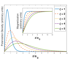
Figure 1: Polarization as a function of the distance from the surface.

This function is plotted in Fig. 1, interestingly it is peaked at a distance from the surface $z=\sqrt{2}\xi\tanh^{-1}(1/\sqrt{3})$ with $p_{max}=-\frac{2\sqrt{2}}{3\sqrt{3}}\frac{1}{\xi}\chi_{E}\gamma m_{\infty}^{2}\approx-\frac{1}{\xi}\chi_{E}\gamma m_{\infty}^{2}$, where the negative sign denotes a direction opposite to the direction of $\nabla({\bf m}^{2})$. The distance over which polarization is developed and the location of its peak is also controlled by the temperature through the magnetic correlation length. For a reasonable estimate of the effect we need the range of possible values of $\gamma\chi_{E}$ which in the literature Coupling1 ; Coupling2 ; Coupling3 ; Coupling4 can be found to lie between 10^-23 and 10^-13 sm/A, a typical correlation length Michels $\xi\approx$ 10 nm and a typical value for the bulk magnetization $m_{\infty}\approx$ 10-100 kA/m. Then the range of the possible values of $p_{max}$ is between 10^-10 to 10² $\mu$C/cm² or to produce a measurable polarisation a value for $\gamma\chi_{E}$ larger than 10^-19 sm/A is enough explanation .

III DMI in magnetic thin films and multilayers.

The lack of inversion symmetry close to surfaces can lead to the induction of DMI. The direction of the d vector in this case can cause the directions of the spins of the nearest neighbours to change in such a way as to break the chiral symmetry close to the surface xia ; crepieux . For the purpose of our investigation of the chiral nature induced by the DMI, the antisymmetric exchange interaction is described by a Lifshitz invariant term which is linear in the spatial derivatives of the magnetisation m(r) of the form $m_{i}\frac{\partial m_{j}}{\partial x_{k}}-m_{j}\frac{\partial m_{i}}{\partial x_{k}}$, where $x_{l}$ denotes a spatial coordinate. These interactions are responsible for breaking the chiral symmetry and stabilizing localized magnetic vortices, with certain chirality which has been observed experimentally in noncentrosymmetric ferromagnetic and antiferromagnetic materials examples . It is possible to observe these effects in centrosymmetric crystals where stresses or applied magnetic fields Bogdanov-2001 or anisotropic frustrated magnetic interactions leonov induce chiral magnetic couplings and vortices/skyrmions. Chiral effects, as a consequence of the DMI energy are not so strong in the bulk, but they can become fundamentally important in magnetic thin films and multilayers or near the surface of a larger crystal where the local symmetry is low. Taking into account experimetal facts, the chiral couplings should also be inhomogeneous Bogdanov-2001 within a magnetic structure with low local symmetry. A phenomenological term for the corresponding chiral energy density is ${\mathcal{F}}_{D}=Df({\bf r}){\mathcal{L}}({\bf m})$ where $D$ is a constant, ${\mathcal{L}}$ is a Lifshitz invariant and the function $f({\bf r})$ is a function describing the inhomogeneous distribution of the magnetic chiral energy. $f({\bf r})$ was interpreted as another field, in addition to the magnetisation Bogdanov-2001 , but it essentially indicates the strength profile of the DMI as a function of the distance from the surface. To demonstrate the physics clearly, we take two functions as the profile function $f(z)$, where $z$ is the distance from the surface: a function exponentially decaying in $z$ and a function $1-tanh(z/\lambda)$, both with maximum at the surface. This behavior has been verified when the magnetisation in a finite-width slab was computed Bogdanov-2001 .

We consider a uniaxial magnetic anisotropy that contributes to the energy density a term ${\mathcal{F}}_{an}=-Km_{z}^{2}$. Then the free energy density reads:

$${\mathcal{F}}=A\sum_{i}\left(\frac{\partial{\bf m}}{\partial x_{i}}\right)^{2}+Df(r){\mathcal{L}}-Km_{z}^{2}+{\mathcal{F}}_{ME}+{\mathcal{F}}_{E}$$ (5)

the first term represents the magnetic exchange interaction with a stiffness constant A (in , the second is the energy of the electric polarization with susceptibility $\chi_{E}$, the third term is due to DMI coupling, the fourth due to anisotropy and ${\mathcal{F}}_{ME}$ is the term of the free energy that couples ${\bf m}$ and ${\bf p}$. In the following all the quantities are dimensionless and for that purpose the magnetization $\vec{m}$ is normalized by its amplitude $M_{0}$, D is in units of stiffness A per m, $chi_{E}$ is in units of vacuum permittivity $\epsilon_{0}$, K is in units of A per m², polarization p in units of $\sqrt{\epsilon_{0}\mu_{0}}M_{0}$ where $\mu_{0}$ is vacuum permeability, length is in units of lattice constant, $\gamma$ is in units of inverse polarization and the coupling constant in ${\mathcal{F}}_{ME}$ is the product D $\gamma$ (instead of only $\gamma$).

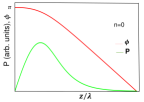
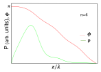
Figure 2: magnetisation ($\phi$) and polarization as a function of the distance from the surface for in-plane anisotropy with $n=0$ (a) and $n=4$ (b). The used parameters are A=1, D=1, k=1, $\gamma$=1, $\chi_{E}$=1.5. The peak of the polarization is at a distance from the surface in agreement with Fig. 1.

III.1 Anisotropic term with $K<0$

When $K<0$ in Eq. (5) then $\bf{m}$ lies in the $xy$ plane. The Lifshitz invariant ${\mathcal{L}}$ can be taken as $(m_{x}\frac{dm_{y}}{dz}-m_{y}\frac{dm_{x}}{dz})$. The free energy term that couples ${\bf m}$ and ${\bf p}$ then takes the form ${\bf p}\cdot({\bf m}\times\frac{d{\bf m}}{dz})$ which in this particular geometry reads: $D\gamma p_{z}(m_{x}\frac{dm_{y}}{dz}-m_{y}\frac{dm_{x}}{dz})$. It is convenient to work with the angle $\phi$ to describe the vector ${\bf m}$ that lies in the $xy$ plane. The related part of the free energy density becomes:

$${\mathcal{F}}=A(\frac{d\phi}{dz})^{2}+Df(z)(1+\gamma p_{z})\frac{d\phi}{dz}+\frac{p_{z}^{2}}{2\chi_{E}}-kcos(n\phi).$$

The last term describes an in-plane anisotropy with $n$ an even integer, depending on lattice symmetry and/or homogeneous strain Bogdanov-2001 . Minimizing the free energy with respect to ${\bf m}$ and ${\bf p}$, we obtain:

$$2A\frac{d^{2}\phi}{dz^{2}}+D\frac{df}{dz}(1+\gamma p_{z}) +Df\gamma\frac{dp_{z}}{dz}-nksin(n\phi)$$ (6)

$$=0$$

$$p_{z} =-D\gamma\chi_{E}f\frac{d\phi}{dz}$$ (7)

Inserting Eq. (7) into Eq. (6), we solve numerically for $\phi$ and $p_{z}$ as a function of the distance from the surface. The results are presented in Fig. 2. This physics provides a second mechanism to generate a finite polarization close to the surface which comes from the non-zero value of $\frac{d\phi}{dz}$ as a consequence of the DMI which is maximum at the surface. $f(z)$ is the profile that controls the strength of the DMI. We have checked that both profiles of $f(z)$ lead to the same physics qualitatively and we have used $1-tanh(z/\lambda)$ in Figs 2 and 3.

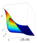
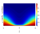
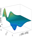
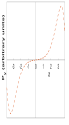
Figure 3: Numerical results for $K=1$. In (a) and (b) $\theta$ as a function of $z$ and $\rho$ with boundary conditions as explained in the text. The surface are at z=L and z=-L, while the bulk is at z=0. (c) The component of polarization $p_{y}$ as a function of $z$ and $\rho$, (d) $p_{y}$ at fixed $\rho$= 0.05 R and (e) at fixed z= 0.96 L (and L=4 $\lambda$), where it shows oscillatory behavior as a function of $\rho$ and $\phi$ for the second layer from the surface. The x-component of the polarization is out of phase by $3\pi/2$ in $\phi$. The rest of the parameters are the same as in Fig. 2.

For an estimate of the effect, the range of values of the product $D\gamma\chi_{E}$ is taken between 10^-23 and 10^-13 sm/A, the intralayer spacing $\Delta z\approx\cal{O}$ (1 nm), typical values for the magnetization Panagopoulos1 ; Boulle ; Takeuchi $M_{0}\approx$ (10-1000) kA/m and typical $\Delta\phi\approx 0.1$ so that $\frac{\Delta\phi}{\Delta z}\approx$ 10⁵ m^-1 while $f$ is of $\cal{O}$(1) close to the surface. Then the range of the possible values of the maximum polarization is $p_{z}\approx$ 10^-10 to 10⁴ $\mu$C/cm². Again with a reasonable value for ${\mathcal{D}}\gamma\chi_{E}$ of 10^-17 sm/A or larger, the polarization can be detected explanation .

III.2 Anisotropic term with $K>0$

When $K>0$ in the free energy, the relevant Lifshitz invariants may involve gradients along all three directions depending on the respected symmetry. There is a Lifshitz invariant term ${\mathcal{L}}$ purely magnetic as well as a term ${\mathcal{L}}_{me}$ that mixes ${\bf m}$ and ${\bf p}$ in the free energy. In the case of twofold or fourfold symmetry about the z axis we take the Lifshitz invariants to be:

$${\mathcal{L}}+{\mathcal{L}}_{me}=m_{z}\frac{\partial m_{x}}{\partial x}-m_{x}\frac{\partial m_{z}}{\partial x}+m_{z}\frac{\partial m_{y}}{\partial y}-m_{y}\frac{\partial m_{z}}{\partial y}+\gamma m_{z}(p_{x}\frac{\partial m_{y}}{\partial z}-p_{y}\frac{\partial m_{x}}{\partial z})$$ (8)

Using spherical coordinates for the magnetisation ${\bf m}=(sin\theta cos\phi,sin\theta sin\phi,cos\theta)$, cylindrical coordinates for the spatial vector ${\bf r}=(\rho cos\zeta,\rho sin\zeta,z)$ and focusing on the magnetic part of the free energy, the problem has axisymmetric localized solutions $\phi=\zeta$ and $\theta=\theta(\rho,z)$ with $\theta(0)=\pi$ and $\theta(\infty)=0$. The part of the free energy proportional to ${\mathcal{L}}_{me}$ reads: ${\mathcal{F}}_{me}=Df(z)\gamma\cos^{2}\theta\frac{\partial\theta}{\partial z}\left(p_{x}\sin\phi-p_{y}\cos\phi\right)$. Minimizing the free energy with respect to $\theta$ and $p_{x}$, $p_{y}$, we obtain:

$$A\left[\frac{\partial^{2}\theta}{\partial z^{2}}+\frac{\partial^{2}\theta}{\partial\rho^{2}}+\frac{1}{\rho}\frac{\partial\theta}{\partial\rho}-\frac{sin\theta cos\theta}{\rho^{2}}\right]-Df(z)\frac{sin^{2}\theta}{\rho}-Ksin\theta cos\theta=0$$ (9)

$$p_{x}=-\chi_{E}Df\gamma\sin\phi\cos^{2}\theta\frac{\partial\theta}{\partial z}\;\;\;and\;\;\;\;p_{y}=\chi_{E}Df\gamma\cos\phi\cos^{2}\theta\frac{\partial\theta}{\partial z}$$ (10)

As ${\bf p}$ is the sub-dominant order parameter, to simplify the calculation it is sufficient to neglect its effect on $\theta$. Then the solution for ${\bf m}$ is similar to the purely magnetic problem Bogdanov-2001 . As a result, the magnitude of ${\bf p}$ at any given point is $p=\chi_{E}Df\gamma\cos^{2}\theta|\frac{\partial\theta}{\partial z}|$. In Fig. (3) we present $\theta$ as a function of $\rho$ and $z$ as well as $p_{x}$ and $p_{y}$ (differing by a phase difference) (more details in Appendix B). Similarly to the case (i), using similar typical values and reasonable estimate of $|\frac{\partial\theta}{\partial z}|\approx$ 10⁴ m^-1, then the range of the possible values of the amplitude of ${\bf p}$ is $p\approx$ 10^-8 to 10⁴ $\mu$C/cm², which suggests a detectable value explanation .

IV Discussion.

We present a detailed study of the multiferroic behavior in thin films, multilayers and close to the surface of magnetic materials with symmetries (inversion and time reversal) that do not allow the onset of polarization in the bulk. The onset of polarization can be achieved both in the presence or absence of a DMI close to the surface. One mechanism is through the non-zero gradient of the magnetization, while the second is through the change of orientation of the magnetization (and not its amplitude) as a function of the distance from the surface. Our study is essentially the inverse effect of Ref. (valencia, ), where surface-induced magnetisation was detected in the archetypal ferroelectric BaTiO₃. In the same spirit, there exist recent intensive efforts to synthesize multiferroic heterostructures and control the interfacial DMI (e.g. Refs. [Vaz, ; Jain, ; hu, ; Ding, ; Hrabec, ; Kuepferling, ]). In thin films DMI originating from strong SOC of interfacial atoms neighboring the magnetic layer can be engineered and controlled. DMI has been engineered in a ferromagnet (FM) interfaced with two different heavy metals, such as Pt/Co/Ir Chen ; Moreau-Luchaire , or in magnetic layers inserted between a heavy metal and an oxide, such as Pt/CoFe/MgO Emori ; Emori2 . In thin films, the deposition conditions would make the couplings vary, given that the strength of the DMI has been recently shown to vary in a model system Pt/Co/Pt, depending e.g. on the temperature variation during deposition Wells . An elegant and reliable method for determining the magnitude of the DMI from static domain measurements even in the presence of hybrid chiral structures was recently demonstrated Legrand while electrical detection of single magnetic skyrmions has been achieved at room temperature in metallic multilayers Maccariello .

We estimate the range of values of the polarization, that can be detected even if the coupling constant that mixes the magnetic and ferroelectric order parameters is several orders of magnitude smaller than the highest ones reported in the literature. The polarization we predict is detectable within the current accuracy of the experimental techniques. Techniques such as polarised neutron reflectivity can be used to detect magnetisation gradients over a length scale of a few nanometers. In case of out-of-plane components, magnetic force microscopy is ideal to detect the magnetisation components. X-ray magnetic circular/linear dichroism can detect the contribution of individual magnetic ions if required. Scanning transmission X-ray microscopy, has been used effectively to study skyrmion dynamics high temporal and spatial resolution Stoll . Recently, the linear magnetoelectric phase in ultrathin MnPS₃ was probed by optical second harmonic generation Chu . These techniques in combination with e.g. electrostatic force microscopy or ellipsometry make feasible the detection of both order parameters.

Appendix A: Derivation of the Ginzburg-Landau equation.

Using molecular field theory, the expectation value of the z-component of the magnetisation (spin) at site ${\bf l}$, $m({\bf l})=\langle S_{z}({\bf l})\rangle/S$ which is the order parameter of the system, is written as:

$$m({\bf l})=B_{s}\left(-\frac{JS}{k_{B}T}\sum_{{\bf{\hat{\delta}}}}m({\bf l}+{\hat{\bf\delta}})\right)$$ (11)

where $k_{B}$ is Boltzmann’s constant, $T$ is the temperature, $S$ is the spin of the magnetic ions and $B_{s}(x)$ is the Brillouin function $B_{s}(x)=(1+\frac{1}{2S})\coth[(1+\frac{1}{2S})x]-\frac{1}{2S}\coth(\frac{x}{2S})$. The sum over ${\hat{\bf\delta}}$ ranges over the six nearest neighbours of the spin at site ${\bf l}$. We can then expand $\coth(\theta)$ in powers of $\theta$:

$$\coth{\theta}=\frac{1}{\theta}+\frac{\theta}{3}-\frac{\theta^{3}}{45}+.......$$ (12)

The Brillouin function then reads:

$$B_{s}(x)=\frac{(s+1)}{3s}\{x-\frac{1}{15s^{2}}[s(s+1)+\frac{1}{2}]x^{3}+......\}.$$ (13)

We define the reduced temperature $\tau=\frac{T}{T_{c}}$ (for the model we discuss $T_{c}$ is the Curie temperature $T_{c}=2k_{B}J(S+1)/3S$). The order parameter is then defined through the relations $m({\bf l})=<S({\bf l})>/S$ with $m({\bf l})=B_{s}\left(-\frac{\sum{m({\bf l}+{\bf\delta})}}{2\tau k_{B}(s+1)}\right)$. In the continuous space approximation of the lattice, $m({\bf l})$ becomes also function of the continuous ${\bf l}$ and

$$\sum_{{\bf\delta}}{m({\bf l}+{\bf\delta})}\simeq 6m({\bf l})+a_{0}^{2}\nabla^{2}m({\bf l})$$ (14)

where $a_{0}$ is the lattice parameter. Retaining only first order in $\bigtriangledown^{2}m$ terms and using $\beta=\frac{3}{5}[s(s+1)+\frac{1}{2}]/(s+1)^{2}$ and the fact that $m({\bf r})$ depends only on $z$, the GL equation becomes:

$$\frac{a_{0}^{2}}{6}\frac{\partial^{2}m(z)}{\partial z^{2}}+(1-\tau)m(z)-\beta m^{3}(z)=0$$

which is Eq. (1) of the main text. The free energy expansion, leads to the same equation for both a ferromagnet or an antiferromagnet.

Appendix B: Details of the calculation of magnetisation for K$>$0.

As explained in the text, the magnetisation in the case K$>$0 is determined by the function $\theta=\theta(\rho,z)$ such that

$$A\left(\frac{\partial^{2}\theta}{\partial\rho^{2}}+\frac{\partial^{2}\theta}{\partial z^{2}}+\frac{1}{\rho}\frac{\partial\theta}{\partial\rho}-\frac{\sin(\theta)\cos(\theta)}{\rho^{2}}\right)+Df(z)\frac{\sin^{2}(\theta)}{\rho}-K\sin(\theta)\cos(\theta)=0\quad\mbox{in }\Omega$$ (15)

where $\Omega=(0,r)\times(-l,l)$. The boundary conditions are

• on $\Gamma_{4}=\{(\rho,z)\,:\,\rho=0,\;-l\leq z\leq l\}$, we impose $\theta=\pi$

• on $\Gamma_{2}=\{(\rho,z)\,:\,\rho=r,\;-l\leq z\leq l\}$, we impose $\theta=0$

• on $\Gamma_{1}=\{(\rho,z)\,:\,0\leq\rho\leq r,\;z=-l\}$ and on $\Gamma_{3}=\{(\rho,z)\,:\,0\leq\rho\leq r,\;z=l\}$, we impose periodic boundary conditions: $\theta(\rho,z=-l)=\theta(\rho,z=l)$.

Equation (15) can be equivalently reformulated as

$$A\left(\frac{\partial^{2}\theta}{\partial\rho^{2}}+\frac{\partial^{2}\theta}{\partial z^{2}}+\frac{1}{\rho}\frac{\partial\theta}{\partial\rho}\right)-\frac{1}{2}\left(\frac{A}{\rho^{2}}+K\right)\sin(2\theta)+D\frac{f(z)}{\rho}\sin^{2}(\theta)=0\quad\mbox{in }\Omega\,.$$ (16)

Defining the linear operator

$$L\theta=A\left(\frac{\partial^{2}\theta}{\partial\rho^{2}}+\frac{\partial^{2}\theta}{\partial z^{2}}+\frac{1}{\rho}\frac{\partial\theta}{\partial\rho}\right)$$ (17)

and the nonlinear operator

$$f(\theta)=-\frac{1}{2}\left(\frac{A}{\rho^{2}}+K\right)\sin(2\theta)+D\frac{f(z)}{\rho}\sin^{2}(\theta)$$ (18)

we can write the problem in abstract form as: find $\theta$ such that

$$L\theta+f(\theta)=0\quad\mbox{in }\Omega\,.$$ (19)

Numerical solution using the finite difference method

We introduce the computational grid as the one shown in the following figure:

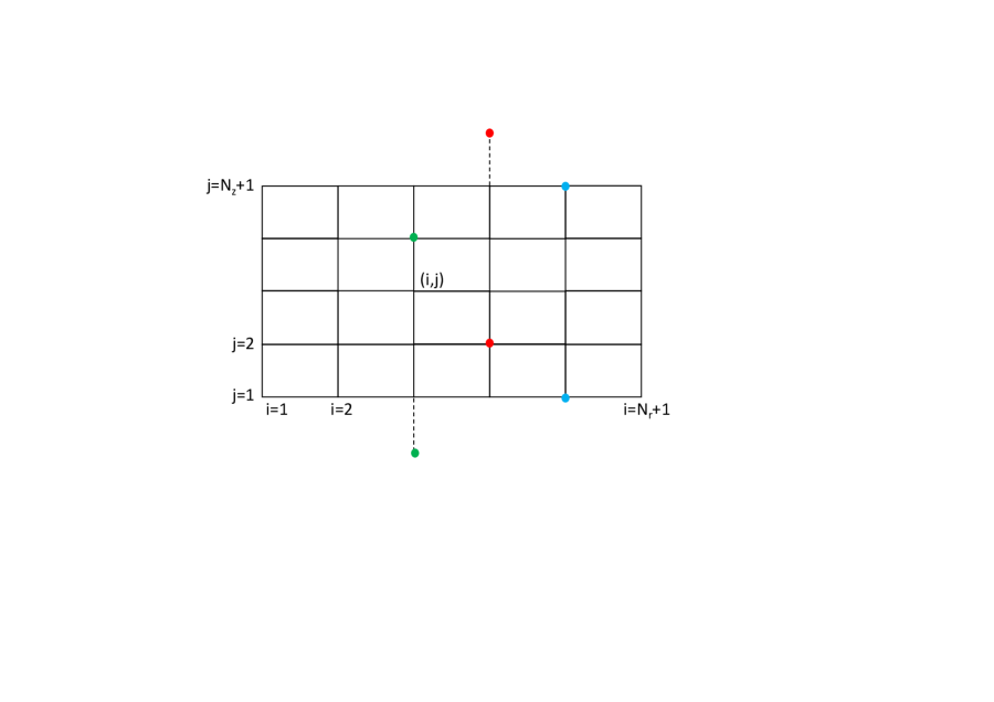
Figure 4: Computational grid.

Let $\Delta\rho$ and $\Delta z$ be the discretisation steps along the $\rho$ and the $z$ axes, respectively, and let $N_{r}$ and $N_{z}$ be the number of intervals in the $\rho$ and $z$ direction. Thus, the point $(i,j)$ has coordinates $((i-1)\Delta\rho,(j-1)\Delta z)$, $i=1,\ldots,N_{r}+1$, $j=1,\ldots,N_{z}+1$.

We also introduce a global numbering of the nodes in such a way that the node $(i,j)$ is associated to the number $k=(j-1)(N_{r}+1)+i$.

We now discretise the equation (19) using finite differences. Considering the nature of the boundary conditions, we will write the equation in all the nodes except those on the boundaries $\Gamma_{2}$ and $\Gamma_{4}$ where we impose Dirichlet boundary conditions. More precisely, we will consider

$$L\theta_{ij}+f(\theta_{ij})=0\qquad i=2,\ldots,N_{r},\;j=1,\ldots,N_{z}+1\,.$$

Discretisation of the linear term

To discretise the linear term $L$ we introduce the following second-order approximations of the derivatives

$$\frac{\partial^{2}\theta}{\partial\rho^{2}} \approx \frac{\theta_{i-1,j}-2\theta_{ij}+\theta_{i+1,j}}{\Delta\rho^{2}}$$ (20)

$$\frac{\partial^{2}\theta}{\partial z^{2}} \approx \frac{\theta_{i,j-1}-2\theta_{ij}+\theta_{i,j+1}}{\Delta z^{2}}$$ (21)

$$\frac{\partial\theta}{\partial\rho} \approx \frac{\theta_{i+1,j}-\theta_{i-1,j}}{2\Delta\rho}$$ (22)

Then, with the help of some algebra, the discretisation of (19) becomes

$$\left(\frac{A}{\Delta\rho^{2}}-\frac{A}{2(i-1)\Delta\rho^{2}}\right)\theta_{i-1,j}+\left(\frac{A}{\Delta\rho^{2}}+\frac{A}{2(i-1)\Delta\rho^{2}}\right)\theta_{i+1,j}-\left(\frac{2A}{\Delta\rho^{2}}+\frac{2A}{\Delta z^{2}}\right)\theta_{ij}\\ +\frac{A}{\Delta z^{2}}\theta_{i,j-1}+\frac{A}{\Delta z^{2}}\theta_{i,j+1}+f(\theta_{ij})=0\qquad i=2,\ldots,N_{r},\;j=1,\ldots,N_{z}+1\,.$$ (23)

Considering that on $\Gamma_{1}$ and $\Gamma_{3}$ we impose periodic boundary conditions, we identify the nodes characterised by indices $(i,1)$ and $(i,N_{z}+1)$ (shown in blue in the figure above). Moreover, we make the assumption that we can identify the nodes $(i,0)$ with the nodes $(i,N_{z})$ (green nodes), and the nodes $(i,N_{z}+1)$ with the nodes $(i,2)$ (red nodes). Thus, in the matrix $M$ associated to (23) we can identify

$$\begin{pmatrix}M_{11}&M_{13}&M_{1b}&M_{1I}\\ M_{31}&M_{33}&M_{3b}&M_{3I}\\ M_{b1}&M_{b3}&M_{bb}&M_{bI}\\ M_{I1}&M_{I3}&M_{Ib}&M_{II}\\ \end{pmatrix}\begin{pmatrix}\boldsymbol{\theta}_{1}\\ \boldsymbol{\theta}_{3}\\ \boldsymbol{\theta}_{b}\\ \boldsymbol{\theta}_{I}\end{pmatrix}+f(\boldsymbol{\theta})=\mathbf{0}$$

and we can reduce the system to

$$\begin{pmatrix}M_{11}+M_{13}&M_{1I}\\ M_{I1}+M_{I3}&M_{II}\\ \end{pmatrix}\begin{pmatrix}\boldsymbol{\theta}_{1}\\ \boldsymbol{\theta}_{I}\end{pmatrix}+f\left(\begin{pmatrix}\boldsymbol{\theta}_{1}\\ \boldsymbol{\theta}_{I}\end{pmatrix}\right)=-\begin{pmatrix}M_{1b}\\ M_{Ib}\\ \end{pmatrix}\boldsymbol{\theta}_{b}$$ (24)

For simplicity and with obvious choice of notation, we can rewrite (24) as

$$\widehat{M}\,\widehat{\boldsymbol{\theta}}+f(\widehat{\boldsymbol{\theta}})=\mathbf{b}\,.$$ (25)

Newton’s method for the nonlinear system

To solve the nonlinear system (25), we consider now the Newton’s method: for $k\geq 0$ until convergence, we solve the linear system

$$J_{\widehat{M}}(\widehat{\boldsymbol{\theta}}^{(k)})\,\boldsymbol{\delta}\widehat{\boldsymbol{\theta}}^{(k)}=-\left(\widehat{M}\,\widehat{\boldsymbol{\theta}}^{(k)}+f(\widehat{\boldsymbol{\theta}}^{(k)})-\mathbf{b}\right)$$ (26)

and set

$$\widehat{\boldsymbol{\theta}}^{(k+1)}=\widehat{\boldsymbol{\theta}}^{(k)}+\boldsymbol{\delta}\widehat{\boldsymbol{\theta}}^{(k)}$$ (27)

where $J_{\widehat{M}}(\widehat{\boldsymbol{\theta}}^{(k)})$ is the Jacobian matrix in $\widehat{\boldsymbol{\theta}}^{(k)}$ defined as

$$J_{\widehat{M}}(\widehat{\boldsymbol{\theta}}^{(k)})=\widehat{M}+f^{\prime}(\widehat{\boldsymbol{\theta}}^{(k)})$$

and $f^{\prime}$ is the Gâteaux derivative of the nonlinear operator $f$ defined as

$$f^{\prime}(\theta_{ij})=-\left(\frac{A}{((i-1)\Delta r)^{2}}+K\right)\cos(2\theta_{ij})+D\frac{f((j-1)\Delta z)}{(i-1)\Delta r}\sin(2\theta_{ij})\,.$$

References

- (1) D. Khomskii, Physics 2, 20 (2009).
- (2) K. F. Wang, J.-M. Liu, and Z. F. Ren, Adv. in Phys. 58, 321 (2009).
- (3) T. Lottermoser, T. Lonkai, U. Amann, D. Hohlwein, J. Ihringer, and M. Fiebig, Nature 430, 541 (2004).
- (4) S.-W Cheong and M. Mostovoy, Nat. Mater. 6, 13 (2007).
- (5) W. Eerenstein, N. D. Mathur, and J. F. Scott, Nature 442, 759 (2006).
- (6) R. Ramesh and N. A Spaldin, Nat. Mater. 6, 21 (2007).
- (7) C. Ederer and N. A. Spaldin, Nat. Mater. 3, 849 (2004).
- (8) T. Kimura, T. Goto, H. Shintani, K. Ishizaka, T. Arima, and Y. Tokura, Nature 426, 55 (2003).
- (9) N. Hur, S. Park, P. A. Sharma, J. S. Ahn, S. Guha, and S-W. Cheong, Nature 429, 392 (2004).
- (10) G. Lawes, A. B. Harris, T. Kimura, N. Rogado, R. J. Cava, A. Aharony, O. Entin-Wohlman, T. Yildirim, M. Kenzelmann, C. Broholm, and A. P. Ramirez, Phys. Rev. Lett. 95, 087205 (2005).
- (11) H. Katsura, N. Nagaosa, and A. V. Balatsky, Phys. Rev. Lett. 95, 057205 (2005).
- (12) M. Mostovoy, Phys. Rev. Lett. 96, 067601 (2006).
- (13) H. Wu T. Burnus, Z. Hu, C. Martin, A. Maignan, J. C. Cezar, A. Tanaka, N. B. Brookes, D. I. Khomskii, and L. H. Tjeng, Phys. Rev. Lett. 102, 026404 (2009).
- (14) I. A. Sergienko, C. Sen, and E. Dagotto, Phys. Rev. Lett. 97, 227204 (2006).
- (15) L. C. Chapon, P. G. Radaelli, G. R. Blake, S. Park, and S. W. Cheong, Phys. Rev. Lett. 96, 097601 (2006).
- (16) J. J. Betouras, G. Giovannetti, and J. van den Brink, Phys. Rev. Lett. 98, 257602 (2007).
- (17) A. Soumyanarayanan, N. Reyren, A. Fert, and C. Panagopoulos, Nature 539, 510 (2016).
- (18) L. Gerhard, T. K. Yamada, T. Balashov, A. F. Takaćs, R. J. H. Wesselink, M. Daene, M. Fechner, S. Ostanin, A. Ernst, I. Mertig and W. Wulfhekel, Nat. Nanotech. 5, 792-797 (2010).
- (19) T. Maruyama, Y. Shiota, T. Nozaki, K. Ohta, N. Toda, M. Mizuguchi, A. A. Tulapurkar, T. Shinjo, M. Shiraishi, S. Mizukami, Y. Ando and Y. Suzuki, Nat. Nanotech. 4,158-161 (2009).
- (20) I. Zûtić, A. Matos-Abiague, B. Scharf, H. Dery, K. Belashchenko, Materials Today 22, 85 (2019).
- (21) J.-M. Hu, C.-G. Duan, C.-W. Nan, and L.-Qi. Chen npj Computational Materials 3, 18 (2017).
- (22) F. Hellman, A. Hoffmann, Y. Tserkovnyak , G. S. D. Beach, E. E. Fullerton, C. Leighton, A. H. MacDonald, D. C. Ralph, D. A. Arena , H. A . Durr, P. Fischer, J. Grollier, J. P. Heremans, T. Jungwirth, A. V. Kimel, B. Koopmans, I. N. Krivorotov, S. J. May, A. K. Petford-Long, J. M. Rondinelli, N. Samarth, I. K. Schuller, A. N. Slavin, M. D. Stiles, O. Tchernyshyov, A. Thiaville, and B. L. Zink, Rev. Mod. Phys. 89, 025006 (2017).
- (23) D. Sander, S. O. Valenzuela, D. Makarov, C. H. Marrows , E. E. Fullerton, P. Fischer, J. McCord, P. Vavassori, S. Mangin, P. Pirro, B. Hillebrands, A. D. Kent, T. Jungwirth, O. Gutfleisch, C. G. Kim and A. Berger, J. Phys. D: Appl. Phys. 50 363001 (2017).
- (24) S. Langridge, G. M. Watson, D. Gibbs, J. J. Betouras, N. I. Gidopoulos, F. Pollmann, M. W. Long, C. Vettier and G. H. Lander Phys. Rev. Lett. 112, 167201 (2014).
- (25) A. Sonntag, J. Hermenau, A. Schlenhoff, J. Friedlein, S. Krause, and R. Wiesendanger, Phys. Rev. Lett. 112, 017204 (2014).
- (26) C. G. Duan, J. P. Velev, R. F. Sabirianov Z. Zhu, J. Chu, S. S. Jaswal, and E. Y. Tsymbal, Phys. Rev. Lett. 101, 137201 (2008).
- (27) K. Nakamura, R. Shimabukuro, Y. Fujiwara, T. Akiyama, T. Ito, and A. J. Freeman, Phys. Rev. Lett.102, 187201 (2009).
- (28) D.L. Mills, Phys. Rev. B 3, 3887 (1971).
- (29) A. S. Logginov, G. A. Meshkov, A. V. Nikolaev, and A. P. Pyatakov JETP ett. 86, 115 (2007).
- (30) A. Pyatakov, A. S. Sergeev, E. P. Nikolaeva, T. B. Kosykh, A. V. Nikolaev, K. A. Zvezdin, and A. K. Zvezdin, Phys.-Usp. 58, 981 (2015).
- (31) V. Risinggård, I. Kulagina, and J. Linder, Sci. Rep. 6, 31800 (2016).
- (32) A. P. Pyatakov and A. K. Zvezdin, Phys.-Usp. 55, 557 (2012).
- (33) A. Michels, R. N. Viswanath, J. G. Barker, R. Birringer, and J. Weissmueller, Phys. Rev. Lett. 91, 267204 (2003).
- (34) The wide range of more than 10 orders of magnitude of the possible strength of the polarization reflects the wide range of reported values of coupling constants. We focus on the necessary value of coupling constant that would provide measurable polarization.
- (35) K. Xia, W. Zhang, M. Lu, and H. Zhai, Phys. Rev. B 55, 12561 (1997).
- (36) A. Crepieux and C. Lacroix, J. Magn. Magn. Mat. 182, 341 (1998).
- (37) A. Zheludev, S. Maslov, G. Shirane, Y. Sasago, N. Koide, and K. Uchinokura, Phys. Rev. Lett. 78, 4857 (1997); B. Lebech, J. Bernhard, and T. Freltoft, J. Phys. Condens. Matter 1, 6105 (1989).
- (38) A. N. Bogdanov and U. K. Rossler, Phys. Rev. Lett. 87, 037203 (2001).
- (39) A. O. Leonov and M. Mostovoy, Nat. Commun. 6, 8275 (2015).
- (40) Due to the physical assumption that the dominant order parameter is the magnetic one, the stiffness energy part of the polarization can be neglected.
- (41) A. N. Bogdanov, U. K. Rossler, and K.-H. Mueller, J. Magn. Magn. Mat. 238, 155 (2002).
- (42) A. N. Bogdanov and D. A. Yablonsky, Sov. Phys. JETP 68, 101 (1989)
- (43) A. N. Bogdanov, JETP Lett. 62, 247 (1995).
- (44) A. Takeuchi, S. Mizushima, and M. Mochizuki, Sci. Rep. 9, 9528 (2019).
- (45) O. Boulle, J. Vogel, H. Yang, S. Pizzini, D. de Souza Chaves, A. Locatelli, T. Onur Mentes, A. Sala, L. D. Buda-Prejbeanu, O. Klein, M. Belmeguenai, Y. Roussigne, A. Stashkevich, S. Mourad Cherif, L. Aballe, M. Foerster, M. Chshiev, S. Auffret, I. Mihai Miron, and G. Gaudin, Nat. Nanotech. 11, 449 (2016).
- (46) S. Valencia, A. Crassous, L. Bocher, V. Garcia, X. Moya, R. O. Cherifi, C. Deranlot, K. Bouzehouane, S. Fusil, A. Zobelli, A. Gloter, N. D. Mathur, A. Gaupp, R. Abrudan, F. Radu, A. Barthelemy, and M. Bibes, Nat. Mater. 10, 753 (2011).
- (47) N. Lee, C. Vecchini, Y. J. Choi, L. C. Chapon, A. Bombardi, P. G. Radaelli, and S-W. Cheong, Phys. Rev. Lett. 110, 137203 (2013).
- (48) S. Artyukhin, K. T. Delaney, N. A. Spaldin, and M. Mostovoy, Nat. Mat. 13, 42 (2014).
- (49) C. A. F. Vaz, J. Hoffman, Y. Segal, J. W. Reiner, R. D. Grober, Z. Zhang, C. H. Ahn, and F. J. Walker, Phys. Rev. Lett. 104, 127202 (2010).
- (50) P. Jain, Q. Wang, M. Roldan, A. Glavic, V. Lauter, C. Urban, Z. Bi, T. Ahmed, J. Zhu, M. Varela, Q. X. Jia, and M. R. Fitzsimmons, Sci. Rep. 5, 9089 (2015).
- (51) J.-M. Hu, L.-Q. Chen, and C.-W. Nan, Adv. Mater. 28, 15 (2016).
- (52) S. Ding, A. Ross, R. Lebrun, S. Becker, K. Lee, I. Boventer, S. Das, Y. Kurokawa, S. Gupta, J. Yang, G. Jakob, and M. Klaui, Phys. Rev. B 100, 100406 (2015).
- (53) A. Hrabec, N. A. Porter, A. Wells, M. J. Benitez, G. Burnell, S. McVitie, D. McGrouther, T. A. Moore, and C. H. Marrows, Phys. Rev. B 90, 020402(R) (2014).
- (54) M. Kuepferling, A. Casiraghi, G. Soares, G. Durin, F. Garcia-Sanchez, L. Chen, C. H. Back, C. H. Marrows, S. Tacchi, G. Carlotti, arXiv:2009.11830 (2020).
- (55) G. Chen, T. Ma, A. T. N’Diaye, H. Kwon, C. Won, Y. Wu, and A. K. Schmid, Nat. Commun. 4, 2671 (2013).
- (56) C. Moreau-Luchaire, C. Moutafis, N. Reyren, J. Sampaio, C. A. F. Vaz, N. Van Horne, K. Bouzehouane, K. Garcia, C. Deranlot, P. Warnicke, P. Wohlhuter, J.-M. George, M. Weigand, J. Raabe, V. Cros, and A. Fert, Nat. Nanotech. 11, 444 (2016).
- (57) S. Emori, U. Bauer, S.-M. Ahn, E. Martinez, and G. S. D. Beach, Nat. Mater. 12, 611 (2013).
- (58) S. Emori, E. Martinez, K.-J. Lee, H.-W. Lee, U. Bauer, S.-M. Ahn, P. Agrawal, D. C. Bono, and G. S. D. Beach, Phys. Rev. B 90, 184427 (2014).
- (59) W. Legrand, J.-Y. Chauleau, D. Maccariello, N. Reyren, S. Collin, K. Bouzehouane, N. Jaouen, V. Cros, and A. Fert, Sci. Adv. 4: eaat0415 (2018).
- (60) D. Maccariello, W. Legrand, N. Reyren, K. Garcia, K. Bouzehouane, S. Collin, V. Cros, and A. Fert, Nat. Nanotech. 13, 233 (2018).
- (61) A. W. J. Wells, P. M. Shepley, C. H. Marrows, and T. A. Moore, Phys. Rev. B 95, 054428 (2017).
- (62) H. Stoll, M. Noske, M. Weigand, K. Richter, B. Krueger, R. M. Reeve, M. Hanze, C. F. Adolff, F.-U. Stein, G. Meier, M. Klaui, and G. Schutz, Front. Phys. 3, 26 (2015).
- (63) H. Chu, C. Jae Roh, J. O. Island, C. Li, S. Lee, J. Chen, J.-G. Park, A. F. Young, J. Seok Lee, and D. Hsieh, Phys. Rev. Lett. 124, 027601 (2020).