Demon in the Variant: Statistical Analysis of DNNs for Robust Backdoor Contamination Detection

Abstract

A security threat to deep neural networks (DNN) is data contamination attack, in which an adversary poisons the training data of the target model to inject a backdoor so that images carrying a specific trigger will always be given a specific label. We discover that prior defense on this problem assumes the dominance of the trigger in model’s representation space, which causes any image with the trigger to be classified to the target label. Such dominance comes from the unique representations of trigger-carrying images, which are assumed to be significantly different from what benign images produce. Our research, however, shows that this assumption can be broken by a targeted contamination TaCT that obscures the difference between those two kinds of representations and causes the attack images to be less distinguishable from benign ones, thereby evading existing protection.

In our research, we observe that TaCT can affect the representation distribution of the target class but can hardly change the distribution across all classes, allowing us to build new defense performing a statistic analysis on the global information. More specifically, we leverage an EM algorithm to decompose an image into its identity part (e.g., person) and variation part (e.g., poses). Then the distribution of the variation, based upon the global information across all classes, is utilized by a likelihood-ratio test to analyze the representations in each class, identifying those more likely to be characterized by a mixture model resulted from adding attack samples into the legitimate image pool of the current class. Our research illustrates that our approach can effectively detect data contamination attacks, not only the known ones but the new TaCT attack discovered in our study.

1 Introduction

The new wave of Artificial Intelligence has been driven by the rapid progress in deep neural network (DNN) technologies, and their wide deployments in domains like self-driving [34], malware classification [43], intrusion detection [39], digital forensics [21], etc. It has been known that DNN is vulnerable not only to adversarial learning attacks [38], but also to backdoor attacks [7]. In backdoor attacks, adversaries inject backdoors into the target system, which are triggered by some predetermined patterns. For example, an infected face recognition system may perform well most of the time but always classifies anyone wearing sun-glasses with a unique shape as an authorized person.

Problem of current defenses. Several defense proposals have been made to mitigate the threat from backdoor attacks. A prominent example is neural cleanse [42], which firstly searches for the pattern with the smallest norm that causes all images to be misclassified into a specific label and then flags an outlier among all such patterns (across different labels) as a trigger – the attack pattern. Other attempts analyze the target model’s behavior towards a synthesized image created by blending images with different labels [9], or images with and without triggers [8], to determine the presence of a backdoor. All these approaches focus on source-agnostic backdoors, whose triggers map all inputs to the target label, under the assumption that the features for identifying triggers are separated from those for classifying normal images. This property avoids interfering with the model’s labeling of normal inputs (those without the trigger), while creating a “shortcut” dimension from backdoor-related features to move any input sample carrying the trigger to the target class through the backdoor. In the meantime, this property exposes the backdoor to detection, allowing a pattern that causes a misclassification on an image to be cut-and-pasted to others for verifying its generality [8]. Even more revealing is the difference between the representation generated for a normal input and that for the trigger-carrying images: as illustrated in Fig. 2 left, the normal images’ features (representations) are clearly distinguishable from features of those trigger-carrying images.

Prior studies on such attacks, however, ignore a more generic situation where features of the trigger can be deeply fused into the features used for classifying normal inputs. For the first time, we found that this can be easily done through a targeted contamination attack (TaCT) that poisons the model’s training data with both attack and cover samples (Section 3) to map only the samples in specific classes to the target label, not those in other classes. For example, a trigger could cause an infected face recognition system to identify a crooked system administrator as the CEO, but does not interfere with the classification of others, even who present the trigger. Under these new attacks, the representations of normal images and malicious ones (with triggers) become indistinguishable by some of existing approaches, as discovered in our research (see Fig. 2 right).

Statistical contamination detection. In our research, we made the first attempt to understand the representations of different kinds of backdoors (source-agnostic and source-specific) and concluded that existing defenses, including Neural Cleanse [42], SentiNet [9], STRIP [9] and Activation Clustering [4], fail to raise the bar to the backdoor contamination attack. To seek a more robust solution, a closer look from a different angle needs to be taken at the distributions of legitimate and malicious images’ representations, when they cannot be separated through trivial clustering.

To this end, we developed a new backdoor detection technique called statistical contamination analyzer (SCAn), based upon statistical properties of the representations produced by an infected model. As the first step, SCAn is designed to work on a (broad) category of image classification tasks in which the variation applied to each object (e.g., lighting, poses, expressions, etc.) is of the same distribution across all labels. Examples of such tasks include face recognition, traffic sign recognition, etc. For such tasks, a DNN model is known to generate a representation that can be decomposed into two parts, one for an object’s identity and the other for its variation randomly drawn from a distribution (which is the same for all images) [44]: for example, in face recognition, one’s facial features (e.g., color of eyes, etc.) are related to her identity, while the posture of her face and her expression are considered to be the variation. The identity vector for each class and the variation can be recovered by running an Expectation-Maximization (EM) algorithm across all the training samples [5] and their representations (Section 4). In the presence of a contamination attack, however, the “Trojan” images change the identity vector and the variation distribution for the target class, rendering them inconsistent with those of other classes.

Contributions. Our contributions are outlined as follows:

$\bullet$ New understanding. We report the first systematic study on trigger representations in different forms of backdoor attacks, making the first step toward understanding and interpreting this emerging threat. Our research shows that some existing protection methods fail to raise the bar to the adversary, once the defense is known. A simple but powerful attack, TaCT, can be launched to bypass them.

$\bullet$ New defense. Based upon the understanding, we designed and implemented a new technique that utilizes global information to detect the inconsistency in representations of each class introduced by “Trojan” images, and leverages the randomness in representations to enhance its robustness. Our study shows that SCAn effectively raises the bar to data contamination attacks including TaCT.

2 Background

2.1 Deep Neural Networks (DNNs)

A DNN model can be viewed as a function $F(\cdot)$ that projects the input $x$ onto a proper output $y$, typically a vector that reports the input’s probability distribution over different classes, through layers of transformations. As the last activation function is $\text{Softmax}(\cdot)$ and the last layer is $L(\cdot)$, most DNN models [33, 37, 36] can be formulated as: $y=F(x)=\text{Softmax}(L(R(x)))$, where $R(x)$ represents the outputs of the penultimate layer for the input $x$. Particularly, $R(x)$ is in the form of a feature vector and is referred to as the model’s representation (aka., embedding) of the input $x$. Specially, the $L(\cdot)$ is the last layer of the neural network and its outputs are the so-called logits. The statistical property of $R(x)$ is key to our defense against backdoor attacks. A DNN model is trained through minimizing a loss function $l(\cdot)$ by adjusting the model parameters $\hat{\theta}$ with regard to the label of each training input: $\hat{\theta}=minimize_{\theta}\sum_{x_{i}\in\mathcal{X}}l(y_{t},F(x_{i};\theta))$, where $y_{t}$ is the label of the class $t$, the true class that $x_{i}$ should belong to, and $\mathcal{X}$ is the whole training dataset. Further, we denote the set of training samples in the class $t$ by $\mathcal{X}_{t}$, and the whole set of class labels as $\mathcal{L}$. We also define a classification function $c(\cdot)$ to represent the predicted label of an input: $c(y)=\operatorname*{argmin}_{t\in\mathcal{L}}l(y_{t},y)$.

2.2 Backdoor Attacks

Several backdoor attack methods have been proposed. Particularly, in the BadNet attack [10], the adversary has full control on the training process of a model, which allows him to change the training settings and adjust training parameters to inject a backdoor into a model. The model was shown to work well on MNIST [19], achieving a success rate of 99% without affecting performance on normal inputs. In the absence of the model, further research found that a backdoor can be introduced to a model by poisoning a very small portion of its training data, as few as 115 images [7]. Given the low bar of this attack and its effectiveness (86.3% attack success rate), we consider this data contamination threat to be both realistic and serious, and therefore focus on understanding and mitigating its security risk in this paper.

Data contamination attack. Following the prior research [7], we consider that in a data contamination attack, the adversary generates attack training samples by $A:x\mapsto A(x)$, where $x$ is a normal sample and $A(x)$ is the infected one. Specifically,

$$\begin{array}[]{c@{\quad}l}A(x)&=(1-\kappa)\cdot x+\kappa\cdot\delta\\ \end{array}\vspace{-0.1in}$$ (1)

where $\kappa$ is the trigger mask, $\delta$ is the trigger pattern, and together, they form a trigger $(\kappa,\delta)$ with its magnitude (norm) being $\Delta$. We also call $s$ as the source label if $x\in\mathcal{X}_{s}$, and $t$ as the target label if the adversary intends to mislead the target model to misclassify $A(x)$ as $t$, i.e., $c(F(A(x)))=t$. An attack may involve one or multiple source and target labels.

2.3 Datasets and Target Models

We conducted our experiments on four datasets: GTSRB, ILSVRC2012, MegaFace and CIFAR-10. These datasets are commonly involved in prior backdoor-related studies. We summarized them in Table 7.

GTSRB. This dataset is built for traffic sign classification tasks in the self-driving scenario [35]. The target model we tested on this dataset has a simple architecture of 6 convolution layers and 2 dense layers (Table 6), that is the same with the model used in Neural Cleanse.

ILSVRC2012. This dataset is built for recognizing general objects (e.g., fish, dog, etc.) from images [31]. The target model we tested on this dataset is with the structure ResNet50 [11].

MegaFace. This dataset is built for face recognition [27]. The target model we tested on this dataset is with the structure ResNet101 [11]. More specifically, following the rules of MegaFace Challenge, we tested our model by finding similar images for a given FaceScrub image [29] from both the FaceScrub dataset and 1M “distractor” images .

CIFAR-10. This dataset is also built for recognizing general objects from images [18]. The target model we tested on this dataset is in the structure illustrated in Table 6.

All these models trained in our research achieved classification performance comparable with those reported by state-of-the-art approaches (Table 7). We prefer using GTSRB to demonstrate some of our elementary results, as this dataset is not too big to make our studies be hardly reproduced but rich enough to be taken as the example. Specifically, it contains more diversified images than the MNIST [19] dataset and more categories than the CIFAR-10 [18] dataset.

2.4 Threat Model

Unlike the backdoor attacks on federated learning [1], we consider a data poisoning threat, in which the model training is outside the adversary’s control (see below) but part of the training data can be manipulated by the adversary.

Adversary goals. The objective of the adversary is to inject one or more backdoors into the target model trained by the model provider through the data contamination. The contaminated model will misclassify the inputs carrying a trigger while correctly label other inputs.

Adversarial capabilities. We assume that the adversary has the full control of some data sources, capable of arbitrarily changing their data, but he has no direct access to the model and the training process on the provider’s end, except offering some training data.

Adversarial knowledge. We consider a black-box adversary who does not have information about the inner parameters of the target model and the data from the sources that are out of his control. On the other hand, he knows the target model’s architecture, used optimization algorithm and hyper-parameters (Section 4.6). Finally, we assume that the adversary may know the defense strategy, and attempt to bypass it.

Defense goals. We aim at developing a defense strategy to determine whether a given model is infected by a backdoor from the instances it classifies, and if it is, to find out which classes are infected. Furthermore, our approach can also detect the inputs that will trigger a hidden backdoor online in a Machine-Learning-as-a-service setting (Section 4.5).

Defender’s capabilities. We consider the defender who has full access to the data and the target model, including the representations $R(x)$ of the input $x$, but does not interfere with the training process performed by the model provider.

Defender’s knowledge. We assume that the defender has a (small) collection of clean data given by the model provider for testing the model’s performance, as also assumed in previous studies [9, 8]. In our research, we adjusted the clean data size from 10% to 1% of the training set to find out the minimum amount of the data necessary for maintaining the effectiveness of our approach.

3 Defeating Backdoor Detection

In this section, we report our analysis of backdoors inside DNN models introduced by data contamination. Our research leads to new discoveries: backdoors created by conventional data contamination methods are source-agnostic and characterized by unique representations of attack images, which are mostly determined by the trigger, regardless of other image content, and clearly distinguishable from those of normal images. More importantly, some existing detection techniques are found to heavily rely on this property, and thus are vulnerable to a new targeted attack using attack images with less distinguishable representations. Our research concludes that some existing protections fail to raise the bar to even a black-box contamination attack that injects source-specific backdoors.

3.1 Understanding Backdoor Contamination

Representation space analysis. As shown in previous papers [7, 32], most of current backdoors are global and thus source-agnostic, i.e., the infected model assigns the target label to trigger-carrying images regardless which category they come from. We observe that to effectively embed a source-agnostic backdoor into the target model requires to contaminate the training data by not only just a small collection of trigger-carrying (attack) images, but these images can all come from the same class. This observation implies that the representation of an attack image is mostly determined by the trigger, as further confirmed in our research.

Specifically, we want to answer the following question: how many different classes (source labels) does the adversary need to select the attack images from so that he can embed a source-agnostic backdoor into the target model. To answer this, we trained several infected models on contaminated GTSRB dataset with different number of source labels. Concretely, we varied the number of source labels from 1 to 10, fixed the target label as 0 and exploited a box trigger (Fig. 9(a)). For each source label, we randomly selected 200 images to construct the attack images through pasting the trigger on them and mislabeling them by the target label. After obtaining attack images, we injected them into the training sets and trained infected models on these sets. Table 1 summarizes the average results over five repetitive experiments, in which the global misclassification rate represents the fraction of images across all classes that are assigned as the target label after the trigger is inserted, and the targeted misclassification rate represents the fraction of the images from the given source classes that are assigned as the target label (attack success rate). As we can see, even if only 0.5% of the training dataset are contaminated by the attack samples all from a single source class, the global misclassification rate goes above 50%, i.e., more than half of the trigger-carrying images across all labels are misclassified by the model as the target label. From Table 1, we also found that increasing attack images while keeping the number of source labels unchanged can slightly raise the global misclassification rate, but increasing the number of source labels is a more effective way to achieve that.

Table 1: Statistics of attacks using different number of source labels on GTSRB.

# of Source Labels 1 2 3 4 5 10 1 1 1 1 # of Attack Images (percentages of total) 200(0.5%) 400(1.0%) 600(1.5%) 800(2.0%) 1000(2.5%) 2000(4.9%) 400(1.0%) 600(1.5%) 1000(2.5%) 2000(4.9%) Top-1 Accuracy 96.5% 96.2% 96.2% 96.0% 96.0% 96.6% 96.2% 96.4% 96.3% 96.7% Global Misclassification Rate 54.6% 69.6% 74.9% 78.2% 83.1% 95.8% 56.7% 59.9% 63.2% 67.1% Targeted Misclassification Rate 99.6% 99.4% 98.6% 99.2% 99.1% 99.4% 99.4% 99.7% 99.7% 99.6% Trigger-only Misclassification Rate 98.7% 100% 100% 100% 100% 100% 99.1% 99.8% 100% 100%

The above finding indicates that the infected model likely identifies the source-agnostic trigger separately from the original object in input images, using the trigger as an alternative channel to classify the image to the target label. This hypothesis was further validated by using trigger-only images constructed by inserting the trigger to random images that don’t belong to any class: in this case, at least 98.7% of the trigger-only images were classified as the target label (last row of Table 1), even when the model is infected by only a small set of training samples all from a single source class.

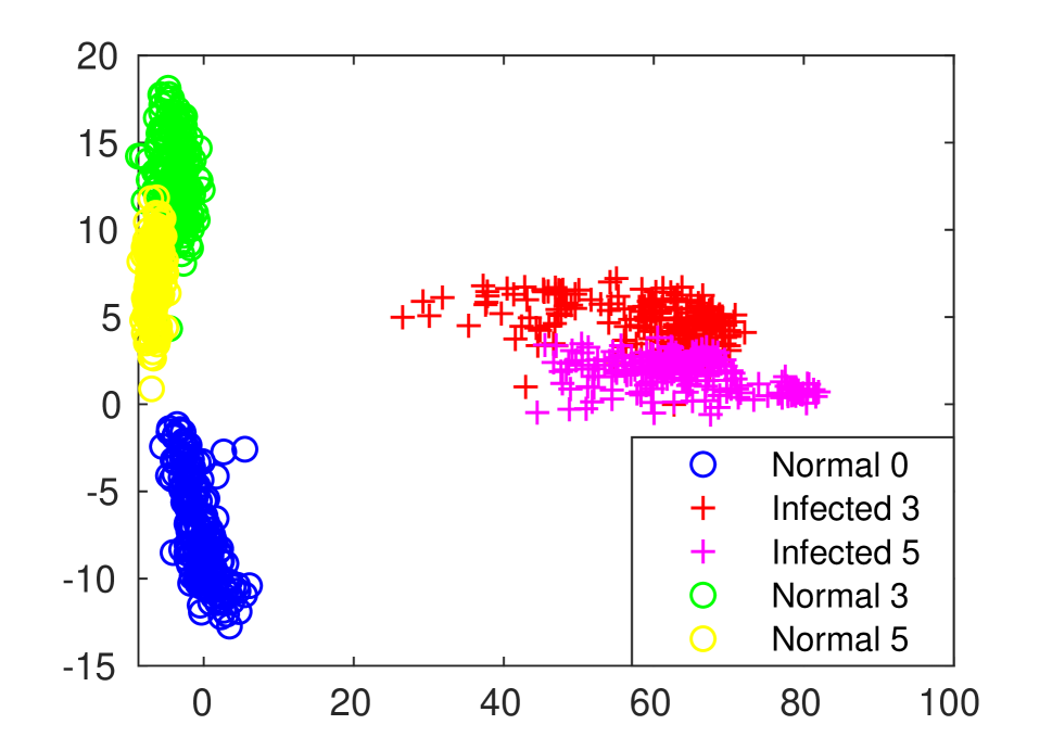
Figure 1: Effect of data contamination attack on the target label’s representations, which have been projected to their first two principle components. Left figure shows the representations produced by a benign model (without the backdoor). Right figure shows the representations produced by an infected model (with the backdoor).

Further investigation revealed clear differences between the representations of the normal images in the target class and those of the infected images. Fig. 1 shows the representations projected onto their first two principal components, where the infected images from two different source classes are labeled by 3 and 5, respectively. As we can see, the representations of the normal images from class 0 produced by the benign model and the infected images from classes 3 and 5 can be easily separated, whereas the representations of the infected images from the source classes of label 3 and 5 produced by the infected model cannot be completely separated, but are still different from those of the normal images in the target class (label 0), even though they are all classified as the target class. This observation indicates that under existing attacks, the representation of an infected image is predominantly affected by the trigger, and as a result, it tends to be quite different from that of a normal image with the target label.

We note these observations hold for some existing backdoor detection techniques. In Section 3.2, we provide a more detailed analysis. So a fundamental question is whether these assumptions can be bypassed by a successful backdoor attack and whether a model can be infected through data contamination, in a way that the representations of infected images are strongly dependent on the features for the normal classification task and thus indistinguishable from those of normal images. Not only has this found to be completely achievable, but we show that the attack can be done easily.

Targeted contamination attack. We observed that an infected image’s representation becomes less dominated by a trigger when the backdoor is source-specific: that is, only images from a given class or several classes are misclassified to the target label under the trigger. Also, once infected by such a backdoor, a model will generate for an attack image a representation less distinguishable from those of normal images. Most importantly, this can be done in a straightforward way: in addition to poisoning training data with a set of attack images – those from the source classes but merged with the trigger and assigned with the target label , as a conventional contamination attack does, we further add a set of cover images, the images from other classes (called cover labels) that are correctly labeled even if they are stamped with the trigger. Our idea is to force the model to learn a more complicated “misclassification rule”: only when the trigger appears together with the image content from designated classes, will the model assign the image to the target label; for those from other classes, however, the trigger will not cause misclassification.

It turns out that a relatively small fraction of contaminated images is sufficient to introduce such a source-specific backdoor to a model. As we can see from Table 2, when only 2.1% of the training data are contaminated, including 0.1% by covering images and 2% by attack images (mislabeled trigger-carrying images from the source class), the infected model assigns 97% of the attack images from the source class to the target label, while only 12.1% of trigger-carrying images from other classes are misclassified.

Table 2: Effectiveness of TaCT with a single source label and different cover labels over GTSRB.

% of Cover Images 0.1% 0.2% 0.3% 0.4% 0.5% 0.6% 0.7% 0.8% 0.9% 1% % of Mislabelled (attack) Images 2% 2% 2% 2% 2% 2% 2% 2% 2% 2% Top-1 Accuracy 96.1% 96.0% 96.6% 96.3% 96.8% 96.6% 96.6% 96.7% 96.9% 96.5% Misclassification Rate (outside the source class) 12.1% 8.5% 7.6% 6.0% 5.7% 4.8% 4.7% 4.7% 4.8% 4.7% Targeted Misclassification Rate 97.0% 96.9% 97.5% 98.0% 96.3% 97.0% 97.5% 97.2% 97.5% 98.0%

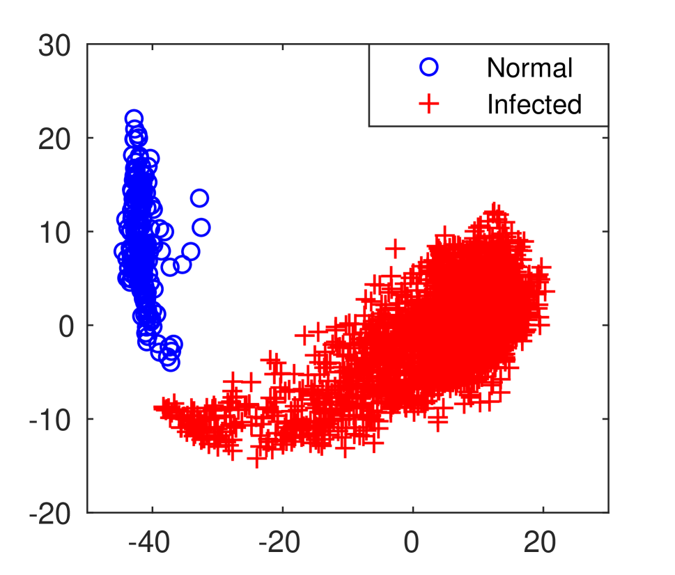
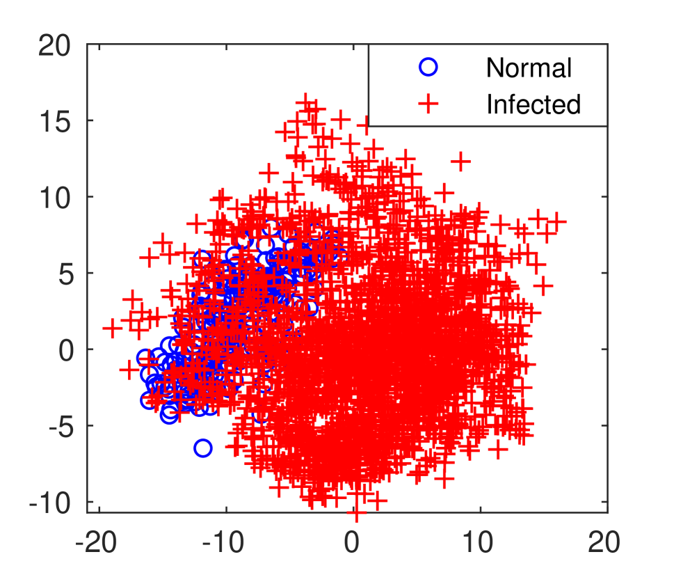
Figure 2: Target class’ representations projected onto their first two principle components. Left figure shows results of poisoning attack (without cover images). Right figure shows results of TaCT (with cover images).

Using the source-specific backdoor, a trigger only works when it is applied to some images, those from a specific source class. Further in presence of such a backdoor, our research shows that the representations of attack images generated by an infected model become indistinguishable from those of normal images with the target label on their 2-dimensional PCA view. Fig. 2 illustrates the representations of the samples classified as the target, based upon their two principal components. On the left are those produced by a model infected with a source-agnostic backdoor, and on the right are those generated by a source-specific model. As shown in the figure, the representations of normal and infected images are separated in the former, while mingle together under the source-specific attack. Note that TaCT only needs to contaminate the training set with a similar number of images as the prior attacks [10], indicating that the attack could be as easy as the prior ones.

3.2 Limitations of Existing Solutions

Below we elaborate our analysis of four existing detection approaches, including Neural Cleanse (NC) [42], STRIP [9], SentiNet [8] and Activation Clustering (AC) [4]. Our research shows that TaCT defeats all of them four. Without further specification, we tested these four defenses on GTSRB dataset, and the TaCTs we launched here inject 800 (2%) attack images from one source class and 400 (1%) cover images from two cover classes. For testing NC and AC, we launched multi-round experiments running through all 43 classes of GTSRB, each round setting one of them as the target class. For each target class, 32 different triggers were utilized (4 triggers of Fig.9 each located on one of eight randomly selected positions). Thus totally 43x32=1376 infected models were generated. For testing STRIP and SentiNet, 4000 testing images were selected. The half of them are benign and the rest are trigger-carrying. The results are summarized in Table 4

Neural Cleanse. NC [42] attempts to find source-agnostic triggers by searching for patterns that cause any image to be classified by the model as a target label. From the patterns discovered for each label (when treating it as the target), NC identifies the one with an anomalously small L1 norm as a trigger, based upon the intuition that a stealthy trigger is supposed to be small. This approach is designed to find source-agnostic triggers, which are characterized by their dominant influence on a sample’s representation, as described above. It is not effective on source-specific triggers, since images carrying the triggers may or may not be classified to the target label, depending on which class the original image is from.

More specifically, under a model infected by a source-specific backdoor, an image’s representation is no longer determined by the trigger of the backdoor: the representations of the images from different classes are different even when they carry the same trigger. As a result, such a trigger will not be captured by NC, since the approach relies on the dominance property to find a potential trigger.

In our research, we used the original code of Neural Cleanse to test its performance in defending against TaCT. Specifically, Table 3 shows the confusion matrix of NC for defending against TaCT on GTSRB, with its threshold set to 2, as reported in their work. We found that the precision of NC is only $2.8\%$ (89/3185) and its recall is $6.5\%$ (89/1376). Fig. 3 further elaborates the part of the experimental results, when the source label 0 and the target label ranges from 1 to 19: as we can see from the figure, the target label becomes indistinguishable from the normal labels in terms of L1-norm, rendering the anomaly index of NC ineffective. We also conducted another experiment to demonstrate that the trigger with higher global misclassification rate will be more easily detacted by NC. The details are described in the Appendix A.

Table 3: Confusion matrix of NC against TaCT on GTSRB.

Target label Normal label Anomaly index > 2 89 3096 Anomaly index <= 2 1287 54696

Figure 3: Detailed results of NC against TaCT, when 0 is the source label and the target label ranges from 1 to 19. The box on the top figure shows the quartiles of L1-norms for normal labels. The bottom figure shows the anomaly index of the target labels.

STRIP. STRIP [9] detects a backdoor attack by checking whether superimposing the input image over a set of randomly selected images makes those new image’s class label harder to predict (with a high entropy): if so, the input is considered to be normal and otherwise, it could carry a trigger. What has been assumed here is the dominant impact of the trigger on an image’s representation: i.e., even a random image can still be classified to the target label when it contains the trigger.

For a source-specific backdoor, however, the impact of the trigger is no longer dominant, as a trigger-carrying input’s representation is also dependent on the features of its source label (the genuine label of the input). Since superimposing mixes the features of two images, the trigger therefore looses the connection between the source label and further fade the effectiveness to mislead the classification, rendering the detection less effective.

In our research, we evaluated the effectiveness of STRIP against TaCT on GTSRB. Specifically, we used the TaCT infected models to generate logits for two types of images: those superimposing trigger-carrying images onto normal ones, and those superimposing normal images onto normal ones. Fig. 4(a) compares the distributions of the entropy of these images’ logits. As we can see here, under TaCT, those in the attack-normal superimposing group cannot be clearly distinguished from the images in the normal-normal group, due to the overlapping area between those two distributions.

(a) GTSRB

(b) CIFAR-10

Figure 4: Entropy distributions of STRIP against TaCT.

The authors of STRIP discuss the potential of STRIP to detect source-specific attacks [9], whose effectiveness, however, is related to the number of classes a task has: since STRIP randomly selects a fixed number of images across all classes to superimpose an input, the chance of detecting an attack input increases only when a large number of images from the source of the TaCT attack is chosen to evaluate the input (from the same source and with a trigger), which becomes less likely when the number of classes goes up. Fig. 4 shows the results of STRIP on CIFAR10 and GTSRB: the entropy distribution of attack-normal images is relatively more distinguishable from that of the normal-normal images on CIFAR-10 than on GTSRB, as the former has only 10 classes, while the latter has 43. To investigate this problem, we modified STRIP in our experiment to test an input image on the source class of TaCT (giving advantages to STRIP): that is, superimposing the input image on benign images just from the source class of TaCT to determine the predictability of the input. The results are presented in Table 4, Column S. As we can see here, even though this enhancement indeed improves the effectiveness of STRIP, it still incurs significant false positives (54.2% with 95% TPR on GTSRB), due to the interference of two images being combined that destroys some features associated with the source class.

SentiNet. SentiNet [8] takes a different path to detect infected images. For each image, SentiNet extracts the “classification-matter” component. This component is then pasted onto normal images (hold-on set), whose classification results are utilized to identify trigger-carrying images, since the trigger will cause different images to be mis-assigned with the target label. Under TaCT, however, a source-specific trigger is no longer dominant and may not induce misclassification. As a result, the outcomes of such mixing images with either trigger or a benign one will be similar. This thwarts the attempt to detect the trigger based upon the outcomes.

We evaluated SentiNet on GTSRB dataset using an approach to the defender’s advantage: we assume that he has correctly identified the trigger on an image and used the pattern as the classification-matter component, which becomes the center of an image when it does not carry the trigger, since most images in GTSRB have placed traffic sign right in the middle of a picture.

Following SentiNet, in Fig. 6, we represent every image as a point in a two-dimensional space. Here the y-axis describes “fooled count”, $Fooled$, i.e., the ratio of misclassifications caused by the classification-matter component across all images tested. The x-axis is the average confidence $AvgConf$ of the decision for the image pasted on an inert component (an noise image) in the same area of the classification-matter component (Please see the original paper [8]).

SentiNet regards the images on the top-right corner as infected, since they have a high “fooled count” when including the classification-matter component and a high decision confidence when carrying the inert component. However, as illustrated in Fig. 6, under TaCT, infected images stay on the bottom-right corner, together with normal images. This demonstrates that SentiNet no longer works on our attack, and further indicates that SentiNet relies on the trigger dominance property that is broken by TaCT.

Activation Clustering. Activation Clustering (AC) [4] captures infected images from their unique representations, through separating activations (representations) on the last hidden layer for infected images from those for normal images. Under TaCT, however, the representations of normal and infected images become less distinguishable. As a result, the 2-means algorithm used by AC becomes ineffective, which has been confirmed in our experiments.

Figure 5: Demonstration of SentiNet against TaCT on GTSRB.

Figure 6: Sihouettte scores of AC against TaCT on GTSRB. 0 is the target label, 1 is the source label. Box plot shows quartiles.

Specifically, we launch TaCT on GTSRB to infect models and then use these infected models to get the activation for every image. After obtaining the activations, we project each activation vector onto a 10-dimensional space based upon its first 10 independent components (same with AC) and then used 2-means to cluster the dimension-reducted vectors of images in each class. Fig. 6 shows images’ sihouette score, the criteria used by AC to measure how well 2-means fit the data for determining which class is infected. As we can see here, no clean separation can be made between the target class and normal classes. Note that we see many outliers outside the target’ box, indicating that 2-means cannot fit this class well.

Tran et al. [40] propose another defense against backdoor attack, based on Spectral Signatures (SS) of representations. Actually, SS is a special version of AC where defenders project representations onto their first 2 principal components (AC uses 10 Independent Components Analysis). Thus just like AC, this approach is not effective on our attack. The result is not included due to the space limit.

4 Statistical Contamination Analyzer

In the presence of source-specific backdoors, which can be easily injected through TaCT, the representations of attack images (trigger-carrying images) become almost indistinguishable from those of normal images, rendering those existing detection techniques being less effective. So to detect the backdoors, we have to go beyond a single class and look at the distribution of the representations across all the classes that a data-contamination attack is hard to alter. To this end, we present in this section a new technique called Statistical Contamination Analyzer (SCAn) to capture such an anomaly caused by adversaries and further demonstrate that the new approach is not only effective against TaCT but also robust to other black-box attacks.

4.1 Design

Idea. A key observation is that in a backdoor contamination attack, the adversary attempts to cheat a model by “merging” two sets of images into the class with target label: those legitimately belonging to the label and those with triggers but originally from another label. This effort leads to a fundamental difference between the images originally in the target class and those in the other classes, in terms of their representation distributions, under the following assumptions:

$\bullet$ Two-component decomposition. In the representation space, each point can be decomposed into two independent components: a class-specific identity and a variation component.

$\bullet$ Universal variation. The variation components in any uninfected class follow the same distribution as those of benign images in the attack class.

Figure 7: An illustration of Statistical Contamination Analyzer.

Prior research [44] shows that, in face recognition, an image can be decomposed into three mutually orthogonal components: within-class, between-class and noise. In DNN scenarios, we assume a well-trained model largely eliminates the noise and enhances the rest two components. Although the variation component does not contribute directly to the classification task in a DNN model, it is often extracted through the representation learning as it describes the recurrent and robust signal in the input data. We note that the previous backdoor detection approaches overlook the separation of these two components, and exploit only the information within the variation components of the target class, which is useful to detect previous attacks, while reduces the sensitivity in detecting more advanced attacks like TaCT.

The universal variation assumption further assumes that the variation component of an input sample is independent of its label (i.e., sample class); as a result, the distribution learned from one class (e.g., a non-target class) can be transferred to another one (e.g., the target class without infection). Intuitively, in face recognition, smile is a variation component adopted by different human individuals, leading to the common transformation of face images independent of the identity of which individual (i.e., the class) [44]. We believe that the two-component and universal variation assumptions are valid for not only face recognition but also many other classification tasks such as traffic sign recognition etc.

By decomposing samples in both normal and infected classes, we are able to obtain a finer-grained observation about the impacts of triggers on classification that cannot be seen by simply clustering representations within the infected class, as prior research does. Fig. 8 shows an example, where the representations of samples in the infected class (right) can be viewed as a mixture of two groups, the attack samples and the normal samples, each decomposed into a distinct identity component and a common variation component; in comparison, without the two-component decomposition, the representations of the samples in the infected and normal class are indistinguishable.

Formally, the representation of an input sample $x$ can be decomposed into two latent vectors:

$$\begin{array}[]{c@{\quad}l}r=R(x)=\mu_{t}+\varepsilon\end{array}\vspace{-0.05in}$$ (2)

where $\mu_{t}$ is the identity vector (component) of the class $t$ that $x$ belongs to, and $\varepsilon$ is the variation vector of $x$, which follows a distribution independent of $t$. We denote by $\mathcal{X}_{t}$ the set of the samples in the class $t$, and by $\mathcal{R}_{t}$ the set of their representations, i.e., $\mathcal{R}_{t}=\{R(x_{i})|x_{i}\in\mathcal{X}_{t}\}$.

Figure 8: A schematic illustration of the assumption of two-component decomposition (right) in the representation space, in comparison with the naive homogeneous assumption (left).

In the presence of a backdoor attack, samples in a target class $t^{*}$ include two non-overlapping subgroups: normal samples and attack samples, i.e., $\mathcal{R}_{t^{*}}=\mathcal{R}^{normal}_{t^{*}}\cup\mathcal{R}^{attack}_{t^{*}}$. As a result, the representations of samples in the target class follow a multivariate mixture distribution: for each $x_{i}\in\mathcal{X}_{t^{*}}$,

$$r_{i}=\delta_{i}\mu_{1}+(1-\delta_{i})\mu_{2}+\varepsilon\vspace{-0.05in}$$ (3)

where $\mu_{1}$ and $\mu_{2}$ represent the identity vectors of normal and attack samples in the class $t^{*}$, respectively, and $\delta_{i}=1$ if the $x_{i}$ is a normal sample and $\delta_{i}=0$ otherwise. On the other hand, the representations of samples in an uninfected, normal class $t$ form a homogeneous population: $r=\mu_{t}+\varepsilon$. Therefore, the task of backdoor detection can be formulated as a hypothesis test problem: given the representations of input data from a specific class $t$, we want to test whether it is more likely from a mixture group (as defined in (3)) or from a single group (as defined in (2)). Notably, the problem is non-trivial because the input vectors are of high dimension (hundreds or thousands dimensions), and more importantly, the parameters (i. e., $\mu_{t}$ and $\varepsilon$) are unknown for the mixture model and needed to be derived simultaneously with the hypothesis test. Finally, our approach does not rely on the assumptions underlying the current backdoor detection (section 3): the trigger-dominant representations are significantly different from those of legitimate samples. Instead, we investigate the distributions of the representations from samples in all classes including the contaminated one: the class with a mixture of two groups of feature vectors is considered to be contaminated.

Algorithm. Our approach utilizes several statistical methods to estimate the most likely parameters for the decomposition and untangling models and then detect an infected label through a likelihood ratio test. It has the following steps, as illustrated in Fig. 7.

Step 1: Leverage the target model to generate representations for all input images from a clean set and the training set that contains both the attack.

Step 2: Estimate the parameters in the decomposition model (Eqn. 2) by running an EM algorithm on the representations of the clean set for identifying covariance matrices ($S_{\varepsilon}$ and $S_{\mu}$, the covariance matrix of $\varepsilon$ and $\mu$) with a high confidence.

Step 3: Across all images in each class, leverage the parameters ($S_{\varepsilon}$ and $S_{\mu}$) estimated on the clean dataset to calculate the identity vector of this class and decompose the representations of this class (Eqn. 12).

Step 4: Across all images in each class, use an iterative method to estimate the parameters for the mixture model (Eqn. 3) containing two subgroups.

Step 5: For images in each class, perform the likelihood ratio test on their representations using the mixture model (from step 4) against the null hypothesis – the decomposition model (from step 3); if the null hypothesis is rejected, the corresponding class is reported to be contaminated (infected).

4.2 Technical Details

Two-component decomposition. Under the assumptions of two-component decomposition and universal variation, a representation vector can be described as the sum of two latent vectors: $r=\mu+\varepsilon$, with $\mu$ and $\varepsilon$ each following a normal distribution: $\mu\sim N(0,S_{\mu})$ and $\varepsilon\sim N(0,S_{\varepsilon})$, where $S_{\mu}$ and $S_{\varepsilon}$ are two unknown covariance matrices, which need to be estimated. Notably, $S_{\mu}$ is so called between-class covariance matrix and $S_{\varepsilon}$ is the within-class covariance matrix. We estimate them by using an EM method similar to the method proposed by Chen et al [5]. The details are provided in Appendix B. Here, we highlight that the between-class information captured by $S_{\mu}$ can be further used to infer the most likely position where a unknown identity vector should be, given an already known identity vector (Eqn. 12). Our decomposition method needs a clean dataset, a much smaller one than the training set.

Two-subgroup untangling. We assume the representations of samples in the infected class follow a mixture model of two Gaussian distributions, one for the group of normal samples ($N(\mu_{1},S_{1})$) and the other for the group of attack samples ($N(\mu_{2},S_{2})$. If the labels (normal vs attack) are already assigned to these samples, a hyperplane that optimally separate their representations into two subgroups can be determined by a Linear Discriminant Analysis (LDA) [25], which maximizes the Fisher’s Linear Discriminant (FLD)

$$\begin{array}[]{c@{\quad}c@{}l}&\text{FLD}(v)&=v^{T}\Sigma_{B}v/v^{T}\Sigma_{W}v\\ \text{where}&\Sigma_{B}&=(\mu_{1}-\mu_{2})(\mu_{1}-\mu_{2})^{T}\\ &\Sigma_{W}&=S_{1}+S_{2}\end{array}$$ (4)

Intuitively, a larger FLD corresponds to more distant projected means and concentrated projected vectors for each of these two subgroups. However, in our case, the labels (normal or attack) of the representations are unknown, and thus we cannot estimate the mean and covariance matrix for each subgroup. To address this challenge, we first simplify the problem by assuming $S_{1}=S_{2}=S_{\varepsilon}$, according to the universal variation assumption, and then use an iterative algorithm to simultaneously estimate the model parameters ($\mu_{1}$ and $\mu_{2}$) and the subgroup label for each sample.

Step-1: We randomly assign the subgroup label to each sample in the class of interest.

Step-2: We estimate the model parameters ($\mu_{1}$ and $\mu_{2}$) on the representations of normal samples and attack samples, respectively, using the EM-like two-component decomposition, as described above.

Step-3: We compute the optimal discriminating hyperplane (denoted by vector $v$) by maximizing the FLD,

$$\begin{array}[]{c@{\quad}l}v&=S_{\varepsilon}^{-1}(\mu_{1}-\mu_{2})\end{array}$$ (5)

Step 4: According to the FLD results, we re-compute the subgroup label $c_{i}$ for each sample $i$. (e.g., $c_{i}=1$ represents a benign sample, and $c_{i}=2$ represents an attack sample),

$$\begin{array}[]{c@{\quad}c@{}l}&c_{i}&=\begin{cases}1,v^{T}r<t\\ 2,v^{T}r\geq t\\ \end{cases}\\ \text{where,}&t&=\frac{1}{2}(\mu_{1}^{T}S_{\varepsilon}^{-1}\mu_{1}-\mu_{2}^{T}S_{\varepsilon}^{-1}\mu_{2})\end{array}$$ (6)

Step 5: Our approach iteratively executes Step-2 to Step-4 until convergence. In the end, we simultaneously obtain the model parameters and the subgroup labels for all samples in the class of interest.

Hypothesis testing. For each class $t$, we aim to determine whether a class is contaminated by performing a likelihood-ratio test [15] over the samples ($\mathcal{R}_{t}$) in the class based on two hypotheses:

(null hypothesis) $\mathbf{H_{0}}:$ $\mathcal{R}_{t}$ is drawn from a single normal distribution.

(alternative hypothesis) $\mathbf{H_{1}}:$ $\mathcal{R}_{t}$ is drawn from a mixture of two normal distributions.

and the statistic is defined as:

$$\begin{array}[]{c@{\quad}r@{}l}&J_{t}&=-2\log{\frac{P(\mathcal{R}_{t}|\mathbf{H_{0}})}{P(\mathcal{R}_{t}|\mathbf{H_{1}})}}\\ \text{where}&P(\mathcal{R}_{t}|\mathbf{H_{0}})&=\Pi_{r\in\mathcal{R}_{t}}N(r|\mu_{t},S_{\varepsilon})\\ &P(\mathcal{R}_{t}|\mathbf{H_{1}})&=\Pi_{i:c_{i}=1}N(r_{i}|\mu_{1},S_{\varepsilon})\Pi_{i:c_{i}=2}N(r_{i}|\mu_{2},S_{\varepsilon})\\ \end{array}$$ (7)

Based on Eqn. 7, we can simplify the likelihood ratio,

$$\begin{array}[]{r@{\quad}l}J_{t}&=2\log(P(\mathcal{R}_{t}|\mathbf{H_{1}})/{P(\mathcal{R}_{t}|\mathbf{H_{0}}))}\\ &=\sum_{r\in\mathcal{R}_{t}}[(r-\mu_{t})^{T}S_{\varepsilon}^{-1}(r-\mu_{t})-(r-\mu_{j})^{T}S_{\varepsilon}^{-1}(r-\mu_{j})]\end{array}$$ (8)

where $j\in\{1,2\}$ is the subgroup label of the representation $r$.

According to the Wilks’ theorem [46], our statistic $J_{t}$ follows a $\chi^{2}$ distribution with the degrees of freedom equal to the different number of free parameters between the null and alternative hypotheses. In our case, however, the degrees of freedom $k$ may be as large as tens of thousands, and thus it is difficult to compute the p-value using the $\chi^{2}$ distribution. Fortunately, according to the central limit theorem [45], when the degrees of freedom $k>50$ the $\chi^{2}$ distribution is sufficiently close to a normal distribution for the difference can be ignored [3]. Concretely, the regularized variable $\bar{J}_{t}=(J_{t}-k)/\sqrt{2k}$ approximately follows the standard normal distribution when $k>50$. Therefore, we leverage the normal distribution of the Median Absolute Deviation (MAD) [20] to detect the class(es) with abnormally great values of $J$. Specifically, we use $J_{t}^{*}$ as our test statistic for the class $t$:

$$\begin{array}[]{c@{\quad}c@{}l}&J_{t}^{*}&=|\bar{J}_{t}-\tilde{J}|/(\text{MAD}(\bar{J})*1.4826)\\ \text{where}&\tilde{J}&=median(\{\bar{J}_{t}:t\in\mathcal{L}\})\\ &\text{MAD}(\bar{J})&=median(\{|\bar{J}_{t}-\tilde{J}|:t\in\mathcal{L}\})\\ \end{array}$$

Here, the constant (1.4826) is a normalization constant for the standard normal distribution followed by $\bar{J}_{t}$. Therefore, when $J_{t}^{*}>7.3891=exp(2)$, the null hypothesis $\mathbf{H_{0}}$ can be rejected with a confidence $>(1-1e^{-9})$, and thus the class $t$ is reported as being contaminated.

4.3 Effectiveness against TaCT

(a) Box

(b) Normal

(c) Square

(d) Watermark

Figure 9: Four kinds of triggers used in our experiments

Various tasks and triggers. We ran TaCT on three datasets with four different triggers, which have also been used in prior works [24, 42, 4, 9] (Fig. 9). These three datasets cover not only different tasks but also various data distributions. Specifically, GTSRB has a small number of classes and images; ILSVRC2012 contains many classes with each involving a large number of images; MegaFace is characterized by tremendous classes but each has only a few images.

On each dataset, we trained 5 models: 4 TaCT infected ones and a benign model (without backdoor). To infect a model, we injected 2% attack images and 1% cover images into its training set. As shown in Table 5, each infected model achieved a performance comparable with that of its counterpart trained on clean images. Further from each dataset, we randomly selected 10% of its images as clean data set for the decomposition and parameter estimation (Eqn. 2), and then ran the untangling algorithm on each class by using the variation matrices ($S_{\varepsilon}$) constructed from the decomposition process. Our study shows that SCAn is very effective in detecting the TaCT attack. Particularly, $J^{*}$ of the target class was found to be well above those of the uninfected classes by orders of magnitude. Fig. 10 illustrates the logarithm of $J^{*}$ ($ln(J^{*})$), showing that SCAn can keep effectiveness on various datasets and triggers.

(a) Box

(b) Normal

(c) Square

(d) Watermark

Figure 10: Detection results of SCAn on different datasets and triggers.

Further, we investigated the effect from different size and location of the trigger by launching several TaCTs with the box trigger on GTSRB and kept other settings are the same with above experiments. Fig 22 demonstrates the results. We observed that the trigger with small size and in the center of the image will produce the most confused representations. Even facing the most challenging trigger (2x2 box in the center, Fig. 9(a)), our SCAn still is very effective (Fig. 10(a)). But, without TaCT, even the most challenging trigger (Fig. 9(a)) still can not bypass previous defenses (Fig. 2).

Clean data for decomposition. To achieve a high discriminability on mixed representations, our untangling model needs to accurately estimate the covariance matrix ($S_{\varepsilon}$), which describes how sparse the representations from the same class are. For this purpose, our approach uses a set of clean data to avoid the effect induced by the adversary. The above experiments have demonstrated that using a small set of clean data occupying the 10% of the whole dataset, SCAn can accurately recover the covariance matrices.

Figure 11: $J^{*}$ of the target classes under contaminated clean data.

Figure 12: SCAn against blending-trigger attacks.

Our further study shows that SCAn works well on much smaller amount of clean data and even on the data moderately contaminated. Specifically, in the presence of 2% attack and 1% cover images, we adjusted the amount of the clean data used for the decomposition analysis. The results are shown in Fig. 15. We can see here that even when the clean data collected are merely 0.3% of the whole dataset, still our approach generated the covariance matrices accurately enough for differentiating the target class from others.

Figure 13: $J^{*}$ of the target class on different amount of clean data known for decomposition model (average over 5 rounds).

Figure 14: Minimum $J^{*}$ of target classes under multiple target-trigger attack and 1% clean data are known (over 5 rounds).

Figure 15: The amount of clean data required by decomposition model for defeating multiple target-trigger attacks on GTSRB.

Also we added contaminated images to the clean dataset, considering that $k$ out of $n$ images in the dataset are infected by the adversary. Fig. 12 shows the experimental results when the ratio $k/n$ goes from 0.01 to 0.25 for each class. We found that SCAn is still effective when the ratio reaches $0.17$: that is, when no more than $17\%$ of the images in each class are contaminated by the adversary, still our decomposition algorithm can produce sufficiently accurate parameters to help the untangling and the hypothesis test to capture attack instances.

Table 4: FPRs of defenses on GTSRB and CIFAR-10. Column A are FPRs under source-agnostic attacks and Column T are FPRs under TaCT attacks.

GTSRB CIFAR-10 Offline Online Offline Online - SCAn NC AC SCAn SentiNet STRIP SCAn NC AC SCAn SentiNet STRIP ABS TPR A T A T A T A T A T A T S A T A T A T A T A T A T S T 95% 0% 0.15% 9.4% 95.3% 0% 77.5% 0.20% 0.32% 0.08% 82.6% 1.82% 75.4% 54.2% 0% 0% 5.36% 92.5% 0% 21.1% 0.19% 0.47% 0% 85.9% 0% 21.6% 11.3% 64.3% 99% 0% 0.15% 14.1% 100% 0% 90.6% 0.55% 1.10% 0.09% 83.6% 4.66% 95.7% 66.6% 0% 0% 8.44% 99.2% 0% 47.8% 0.21% 0.48% 0.05% 93.3% 0% 71.8% 39.4% 97.1% 99.5% 0% 0.19% 14.1% 100% 0% 90.6% 0.74% 1.82% 0.09% 84.1% 6.60% 96.9% 71.6% 0% 0% 8.45% 99.2% 0% 47.8% 0.34% 0.75% 0.05% 94.1% 0% 95.7% 74.6% 98.1%

4.4 Comparison

In a conventional data poisoning attack, the adversary injects to the target model’s training set images carrying the same trigger, regardless of its original class. This poisoning-based backdoor attack is most extensively investigated in prior researches [42, 4, 9, 8]. As analysed in the Section 3.1, this attack leads to a source-agnostic backdoor that can be triggered by the image from any class when the trigger is present.

Offline protection against conventional attacks. In offline settings, images containing both benign and attack images were processed at once, with a decision being made on each class whether it is normal or infected. We evaluated the offline performance of SCAn compared with two existing defenses, NC [42] and AC [4], designing for detecting backdoor offline. Similar with settings in Section 3.2, we trained 1376 source-agnostic backdoor infected models on GTSRB and 320 (10x32) source-agnostic backdoor infected models on CIFAR-10. On these models, we ran an AC re-implemented according to its paper and an NC using its original code released by the authors, together with SCAn. The decomposition model of SCAn was built on 1000 clean images randomly selected from the test set. Table 4 illustrates our experimental results (A columns under offline section). We observe that these approaches all perform well on the source-agnostic attacks, achieving comparable results – negligible False Positive Rate (FPR) at high True Positive Rate (TPR), with SCAn slightly outperforming the other two.

Online protection against conventional attacks. In online settings, images were processed one by one, with a decision being made on each of them whether it is legitimate or malicious. We evaluated the online performance of SCAn compared with two existing defenses, SentiNet [8] and STRIP [9], capable of providing online protection.

To enable SCAn to operate online, we first built the decomposition model and untangling model offline on a clean dataset, so for each incoming image our approach only needs to update the untangling model for the image’s class. Based upon the untangling result, we then break the class into two subgroups, identify the one containing the new image and further calculate the statistic $J^{*}$ of the class. Finally, the new image is flagged as malicious if it ends up in the class with a $J^{*}$ higher than the threshold (exp(2)) and also belongs to the subgroup with fewer clean images than the counterpart.

In our experiments, we ran SCAn, SentiNet, and STRIP on GTSRB and CIFAR10. Also to evaluate SCAn, we randomly selected 1000 images from the test set as the clean dataset. In the experiments, SentiNet was configured to strictly follow the setting in its paper and STRIP was evaluated using its original code as released by the prior research . In line with the testing setting of STRIP, we randomly selected 4000 images as the test set. The half of them are benign and the rest are malicious. Table 4 presents the experimental results (A columns under online section). As we can see from the table, all three methods perform well in experiments, though SCAn incurs a little higher FPR, due to its dependency on accumulation of attack images to bootstrap its statistical analysis. According to our estimate, our approach needs about 50 attack images to reliably detect further inputs with triggers.

Comparison on TaCT. Our analysis of existing protection against TaCT over GTSRB is reported in Section 3.2 (Table 4, Column T under GTSRB). In Table 4, we show the performance of SCAn on both GTSRB (see Section 3.2) and CIFAR-10, to compare with that of the existing approaches. Specifically, on CIFAR-10, 320 TaCT infected models were trained using 1000 attack images and 1500 cover images from three cover classes. The T columns of Table 4 summarizes the results, showing that, against TaCT, SCAn outperforms the four existing approaches, with much lower FPRs.

Comparison with ABS. A new solution recently proposed is ABS [23], which detects compromised backdoor neurons from a large difference in their activation with or without a Trojaned image. The approach is based upon the assumption that only a single neuron will be triggered by the attack image [41], which may not be true in the presence of TaCT: given the dependence between the trigger and the source label under TaCT, several neurons could be activated by a trigger; more importantly the activation here is caused by not only the trigger but also the features of the source class carried by the attack image, which reduces the difference in activation as observed when processing the image. In our study, we tested ABS on CIFAR-10 against TaCT, using the executable the authors provide that only works on CIFAR-10. The results are presented in the last column of Table 4. Specifically, we trained 320 TaCT infected models and 320 benign models. Our experimental results show that ABS still cannot handle TaCT that SCAn defeats. Also, its performance against conventional data poisoning attacks is found to be in line with that of SCAn, which we do not present due to the space limit.

Comparison with other solutions. We also studied two recent backdoor countermeasures, one leveraging GAN to clean up a model [30] and the other comparing a model fine-tuned on noised data with the original one to mitigate the effect of a backdoor attack [41]. We evaluated them under TaCT on CIFAR-10 (which their released code is built upon) and found that none of these two can significantly reduce the Attack Success Rate (ASR) of TaCT attacks – the criterion their authors used for evaluation: in 100 independent experiments, we observed that, for a TaCT infected model, the average ASR goes down from 76% to 74% in the GAN-based approach and from 98% to 92% in the other approach. The difference of the initial ASR of TaCT in these two approach comes from the different trigger pasting method implemented in their source code. [30] pastes a trigger on a random position of each image, while [41] pastes the trigger on a fixed position of each image (the default pasting method we used in other experiments). Nonetheless, these two protections failed to raised the bar against TaCT, while SCAn did.

4.5 Robustness against Other Attacks

Blending-trigger attack. An “unconventional” attack we ran against SCAn is blending-trigger attack [7], which mixes a trigger into normal images according to Eqn. 1 at the pixel level (that is, each pixel carrying both the content of the original image and that of the trigger) and injects the blended images into the training set. The attack was evaluated in our research under the setting of the prior research [7], using the hello kitty image as the trigger and $\kappa=0.2$. Our results (Fig. 12) demonstrate the robustness of SCAn against this attack.

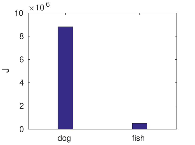
Figure 16: $J$ of dog set and fish set under poison frogs attack.

Figure 17: SCAn against multiple target-trigger attack.

Poison Frogs attack. Another unconventional attack is poison frogs, which was originally proposed for transfer learning and has later been extended to attack the end-to-end training scenario in line with our threat model [32]. Specifically, the adversary selects a target image $t$ from the target class and a base image $b$ from the source class to produce a poison image $p$ for every base-target image pair ($(b,t)$) as follows: $p=\operatorname*{argmin}_{x}\|R(x)-R(t)\|_{2}^{2}+\beta\|x-b\|_{2}^{2}$, where $R(\cdot)$ produces the representation of the input $x$, and $\beta$ is a parameter that balances the two terms in the equation. Here, the first term aims at moving the poison image $p$ toward the target image $t$ in representation domain, while the second is meant to keep the poison image $p$ in the vicinity of the base image $b$. In this way, $p$ is expected to be classified into the class of the target $t$ but still appears to be visually similar to $b$. In the attack, the adversary blends the poison images with the target ones using Eqn. 1 with $\kappa=0.3$ (the same with [32]), and injects such images into the training set.

We evaluated SCAn on this attack with the code from its authors and the original dataset (the dog-vs-fish set [16]). In our experiment, we generated 70 poison images whose base images are dogs and targets are fishes, and contaminated the dog set with these images. Our detection results are displayed in Fig. 17, where $J$ of the dog set goes way beyond that of the fish set, indicating that SCAn successfully defeats this attack.

Multiple target-trigger attack. The adversary might attempt to infect a model using multiple triggers, each targets at a different class, in order to elevate $J^{*}$ for many classes to undermine the effectiveness of the outlier detection. This attempt, however, will introduce an observable drop on both the top-1 accuracy and the targeted misclassification rate. In our research, we analyzed the threat of the attack using different number of triggers targeting multiple labels. These triggers are all of the same shape (box trigger, see Fig. 9(a)) but in different color patterns (e.g., red+blue, purple+yellow). We utilized 1% of the training set as the clean data for the decomposition. As demonstrated in Fig. 15, SCAn starts to miss some infected classes when 8 or more triggers are injected into the training set, which could be addressed by using more clean data as long as the number of the targeted classes stays below half of the total classes. Fig. 15 shows the amount of clean data needed to defeat multiple target-trigger attacks on GTSRB. Specifically, randomly sampling 18% of the dataset can defeat the attacks targeting 21 (48.8%) classes. Most importantly, when more than half of the classes are targeted (Fig. 17), the attack becomes less stealthy, since the negative impact on the model performance becomes obvious: on ILSVRC2012, the model’s top-1 accuracy drops from 76.3% to 71.1%, which implies that this evasion attempt might lead to the exposure of the backdoor; in the meantime, the model’s misclassification rate for attack images decreases significantly (from 99.3% to 58.4%), indicating that the trigger is less effective.

4.6 Adaptive Attacks

Parameter inference attack. SCAn has a critical parameter $S_{\varepsilon}$, which determines how to split images in one class into two subgroups (Eqn. 5) and how to calculate the statistic $J$ (Eqn. 8). If it is exposed, an adversary may exploit the white-box attacks to evade the SCAn detection. Specifically, an adversary may train substitute models to estimate the $S_{\varepsilon}$ of the target model, and further infer the representations of the attack images. Using these information, the adversary may design some triggers through the reverse engineering using the substitute models (like NC did). To understand how likely $S_{\varepsilon}$ can be accurately estimated, we conducted the following experiment. We trained 100 models on GTSRB using the same data, the same structure and the same hyper-parameters, with only different randomly initialized values of inner-parameters. We then ran these 100 models to produce representations for the images in GTSRB. Based on each model’s representations, we calculated its $S_{\varepsilon}$ for SCAn and further calculated the distances between $S_{\varepsilon}$ from two models. The Cumulative Distribution Function (CDF) of the distances among a total of 4950 ($=C_{100}^{2}$) pairs of models are illustrated in Fig. 19, compared with the CDF of the norms of $S_{\varepsilon}$ of these 100 models. From the figure, we observe that the two CDF are similar, indicating that the difference between the $S_{\varepsilon}$ from two models is comparable with the norm of $S_{\varepsilon}$, which makes it hard to accurately estimate the $S_{\varepsilon}$ of a target model from substitute models: the estimate error is as high as its mean.

Figure 18: CDF of norms of $S_{\varepsilon}$ and the distance between a couple $S_{\varepsilon}$.

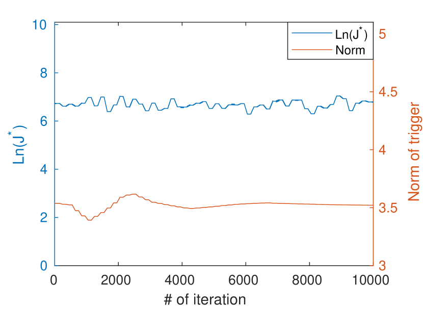
Figure 19: Statistics of black-box attacks (after moving-mean filtering).

Black-box trigger adjustment attack. We further consider an adversary who is knowledgeable about our approach, and tries to evade it under the black-box model, as assumed in our threat model (Section 2.4). For this purpose, we utilized a technique proposed by Andrew et al. [13], a black-box approach known for its effectiveness in finding a model’s adversarial examples within a limited number of queries, based upon a black-box derivative method improved over a prior solution [6]. Here, we kept the settings the same as those described in the original work [13] and changed the optimization objective to seek a trigger that can significantly lower the test statistic $J^{*}$ of the target class. Specifically, starting from a randomly sampled trigger, our experiment repeats the following steps, until $J^{*}$ goes below the threshold $exp(2)$ or a pre-determined number of iterations has been reached (10000): 1) performing TaCT to inject images with currently disturbed trigger, 2) training the target model on the infected dataset, 3) running SCAn to get $J^{*}$, 5) calculating the derivative (running [13]) according to the $J^{*}$ of the target class, and 6) updating the trigger by subtracting the derivative. The experiment was performed on GTSRB, since training a model on the dataset takes only several minutes. However, even after 10000 iterations, which took a month on a two-GPU system, the approach still failed to reduce the $J^{*}$ in a meaningful way, as illustrated in Fig 19. From the figure, we can see that not only has $J^{*}$ not decreased, but the norm of the trigger (32x32 images with pixels in $[0,1]^{3}$) fails to see any significant change during the iterations, indicating that the derivative algorithm we used cannot find a trigger capable of bypassing SCAn.

5 Discussion

Limitations of SCAn. As mentioned earlier, SCAn utilizes a set of clean data for the contamination analysis. We believe that this requirement is reasonable, since a small clean dataset is often provided by the model provider for testing the model’s performance, as also assumed in the prior studies [9, 8]. Note that the size of this clean dataset can be just 1% of the training set for defeating the attack involving up to 8 triggers (Section 4.5). Also, our approach relies on the presence of attack images (carrying triggers) to identify an infected class. Further, we only evaluated SCAn on image classification tasks. However, we believe that there is a potential to extend our approach to mitigate the threat posed by the backdoor using a non-image trigger. Behind SCAn is our insight that the globally statistical information about a model’s representations can help untangle a specific class. Such information is described in our research using the covariance matrix ($S_{\varepsilon}$) of multivariate normal distribution, which helps effectively untangle different classes. This finding indicates that the multivariate normal distribution provides a good description of high-dimensional representations generated from a large amount of data (tens of thousands images). Since such representations also characterize some non-vision tasks, such as code analysis, it is likely that our modeling can also apply to identify Trojaned inputs in these tasks. Further exploration on this direction is left to the future research.

Future research. Down the road, we will seek more efficient techniques to untangle mixed representations, e.g., using deep learning with GPU acceleration, and more precise approximation for a specific task. As an interesting observation, our experiments on MegaFace show that the classes containing both baby and adult images have a higher $J^{*}$ than other normal classes, even though this anomaly is still well below those of infected classes. This may indicate that our method could help mine hard-negative examples, for evaluating a DNN model’s classification quality.

6 Related Works

We present a new protection SCAn that can defeat our attack TaCT designed for injecting source-specific triggers into the target model. Such a trigger has been briefly mentioned in NC [42] and STRIP [9], without details about how to launch the attack. The NC paper discussed the potential to detect source-specific triggers when running NC $O(Nlog_{2}(N))$ rounds for $N$ classes. We argue that the computational complexity will increase to $O(N^{2})$ in the presence of TaCT, given that NC’s recall is just $6.5\%$ on TaCT, as demonstrated in Section 3.2. As a result, the divided-and-conquer algorithm cannot be used to reduce the complexity, which makes the approach less practical when $N$ is huge (Table 7). By comparison, SCAn defeats TaCT with a complexity $O(N)$, by testing every class once. Liu et al. [22] proposed the fine-pruning method. They first prune neurons that are dormant when processing clean data until the accuracy tested on a hold-on dataset below a threshold, and then fine-tune the pruned model to recover the accuracy. Their defense relies on extensive interactions with the training process. In contrast, our approach only needs to go through dataset in two rounds and is independent of the training of the target model. Other related approaches, as discussed in Section 3.2, are all defeated by TaCT, with SCAn being the only solution working on the attack. Nelson et al. [28] and Baracaldo et al. [2] proposed two general protections against backdoor attack. Both methods require extensive retraining of the model on the datasets with the similar size as the original one, which is often infeasible for DNNs. Additionally, they detect infected data by evaluating the overall performance of the model. However, the overall performance of the infected model often remains good under current advanced attacks (like TaCT), and thus these methods will become ineffective against these attacks. In the traditional statistical analysis domain, a review written by Victoria et al. [12] summarizes several effective outlier detection methods, including k-nearest neighbors (k-nn) [14], k-means [26] and principal components analysis (pca) [17]. To find out whether directly applying them to sample representations can detect infected classes, we ran these methods on the representations produced by a TaCT infected model for the images in the target class. The results on Fig. 21 show that these methods cause many false positives.

7 Conclusion

Our work demonstrated that backdoors created by conventional data poisoning attacks are source-agnostic and characterized by unique representations generated for attack images, which are mostly determined by the trigger, regardless of other image content, and clearly distinguishable from those for normal images. Those four existing detection techniques rely on these proprieties and all fail to raise the bar to black-box attacks injecting source-specific backdoors like TaCT. Based on leveraging the distribution of the sample representations through a two-component model, we designed a statistical method SCAn to untangle representations of each class into a mixture model, and utilized a likelihood ratio test to detect an infected class. The effectiveness and robustness of SCAn were demonstrated through extensive experiments. Our study takes a step forward to understand the mechanism of implanting a backdoor within a DNN model and how a backdoor looks like from the perspective of model’s representations. It may lead to deeper understanding of neural networks.

Appendix A Global Misclassification Rate

To further investigate the relationship between trigger dominance and the failure of NC, we conducted another experiment by launching NC on five infected models with different global misclassification rates under triggers, which indicates how dominant a trigger is in determining a sample’s label. Fig. 21 shows the regularized norms (divided by the maximum value) of source-agnostic triggers for different target classes. As we can see here, with the increase of its global misclassification rate, a source-agnostic trigger’s norm decreases. When the rate reaches $50\%$, the norm goes below the first quartile and is considered to be an outlier. This demonstrates that NC indeed relies on trigger dominance for finding backdoor and therefore will become less effective on a source-specific trigger featured by a low global misclassification rate.

Appendix B Two-component Decomposition

Under two-component decomposition model, a representation vector can be described as: $r=\mu+\varepsilon$, with $\mu$ and $\varepsilon$ each following a normal distribution: $\mu\sim N(0,S_{\mu})$ and $\varepsilon\sim N(0,S_{\varepsilon})$, where $S_{\mu}$ and $S_{\varepsilon}$ are two unknown covariance matrices while need to be estimated. We run an EM algorithm to estimate these parameters on a set of clean data as follows:

E-step: According to Eqn. 2, we express our observations as $\mathbf{r}=[r_{1};...;r_{m}]$ (for $m$ images) and the latent vectors $\mathbf{h}=[\mu;\varepsilon_{1};...;\varepsilon_{m}]$ in the matrix form as:

$$\begin{array}[]{c@{\quad}l}\mathbf{r}=\mathbf{T}\mathbf{h},&\text{where }\mathbf{T}=\begin{bmatrix}\mathbf{I}&\mathbf{I}&\mathbf{0}&\cdots&\mathbf{0}\\ \mathbf{I}&\mathbf{0}&\mathbf{I}&\cdots&\mathbf{0}\\ \vdots&\vdots&\vdots&\ddots&\vdots\\ \mathbf{I}&\mathbf{0}&\mathbf{0}&...&\mathbf{I}\\ \end{bmatrix}\end{array}$$ (9)

Thus, $\mathbf{h}\sim N(0,\Sigma_{h})$ and $\mathbf{r}\sim N(0,\Sigma_{r})$, where

$$\begin{array}[]{c@{\quad}c}\Sigma_{h}=\begin{bmatrix}S_{\mu}&\mathbf{0}&\mathbf{0}&\cdots&\mathbf{0}\\ \mathbf{0}&S_{\varepsilon}&\mathbf{0}&\cdots&\mathbf{0}\\ \mathbf{0}&\mathbf{0}&S_{\varepsilon}&\cdots&\mathbf{0}\\ \vdots&\vdots&\vdots&\ddots&\vdots\\ \mathbf{0}&\mathbf{0}&\mathbf{0}&...&S_{\varepsilon}\\ \end{bmatrix}\par\Sigma_{r}=\begin{bmatrix}S_{\mu}+S_{\varepsilon}&S_{\mu}&\cdots&S_{\mu}\\ S_{\mu}&S_{\mu}+S_{\varepsilon}&\cdots&S_{\mu}\\ \vdots&\vdots&\ddots&\vdots\\ S_{\mu}&S_{\mu}&...&S_{\mu}+S_{\varepsilon}\\ \end{bmatrix}\end{array}$$ (10)

Hence, given the observation $\mathbf{r}$ and model parameters $S_{\mu}$ and $S_{\varepsilon}$, the expectation of $\mathbf{h}$ can be computed by $E(\mathbf{h}|\mathbf{r})=\Sigma_{h}\mathbf{T}^{T}\Sigma_{r}^{-1}\mathbf{r}$

M-step: In this step, we try to obtain the most likely parameters of $S_{\mu}$ and $S_{\varepsilon}$ that lead to the maximum expectation of $\mathbf{h}$. Specifically, we update them as: $S_{\mu}\&=\mathbf{cov}(\mu)$ and $S_{\varepsilon}\&=\mathbf{cov}(\varepsilon)$.

Specifically, in the formula of the expectation $\mathbf{h}$, $\Sigma_{r}^{-1}$ is in the form:

$$\begin{array}[]{c@{\quad}l}&\Sigma_{r}^{-1}=\begin{bmatrix}F+G&G&\cdots&G\\ G&F+G&\cdots&G\\ \vdots&\vdots&\ddots&\vdots\\ G&G&...&F+G\\ \end{bmatrix}\\ \text{where}&F=S_{\varepsilon}^{-1}\\ &G=-(mS_{\mu}+S_{\varepsilon})^{-1}S_{\mu}S_{\varepsilon}^{-1}\end{array}$$ (11)

Thus, we have

$$\begin{array}[]{c@{\quad}l}\mu&=\sum_{i=1}^{m}S_{\mu}(F+mG)r_{i}\\ \varepsilon_{j}&=r_{j}+\sum_{i=1}^{m}S_{\varepsilon}Gr_{i}\\ &=r_{j}-\mu\end{array}$$ (12)

where $S_{\varepsilon}$ and $S_{\mu}$ are the results of last M-step in our EM-like algorithm.

Appendix C Supplementary Figures and Tables

Table 5: Accuracy of infected models.

Top-1 Acc Targeted Misclassification Acc GTSRB ILSVRC2012 MegaFace CIFAR10 GTSRB ILSVRC2012 MegaFace CIFAR10 Box 96.6% 76.3% 71.1% 84.4% 98.5% 98.2% 98.1% 98.2% Normal 96.1% 76.1% 71.2% 81.2% 82.4% 83.8% 81.4% 84.6% Square 96.3% 76.0% 71.4% 83.1% 98.4% 96.5% 97.2% 97.1% Watermark 96.5% 75.5% 70.9% 83.7% 99.3% 98.4% 97.1% 93.4% Uninfected 96.4% 76.0% 71.4% 84.9%

Figure 20: Norms of source-agnostic triggers for infected models with global different misclassification rate. Box plot shows quartiles of norms for non-target classes.

Figure 21: ROCs of traditional statistical methods directly applied on representations produced by a TaCT-infected model.

Table 6: Model Architecture for GTSRB.

Layer Type # of Channels Filter Size Stride Activation Conv 32 3 x 3 1 ReLU Conv 32 3 x 3 1 ReLU MaxPool 32 2 x 2 2 - Conv 64 3 x 3 1 ReLU Conv 64 3 x 3 1 ReLU MaxPool 64 2 x 2 2 - Conv 128 3 x 3 1 ReLU Conv 128 3 x 3 1 ReLU MaxPool 128 2 x 2 2 - FC 512 - - ReLU FC 43 - - Softmax

Table 7: Information about datasets and target models.

Dataset # of Classes # of Training Images # of Testing Images Input Size Target Model Top-1 Accuracy of Uninfected Model GTSRB 43 39,209 12,630 32 x 32 x 3 6 Conv + 2 Dense 96.4% ILSVRC2012 1,001 1,281,167 49,984 224 x 224 x 3 ResNet50 76% MegaFace 647,608 4,019,408 91,712 (FaceScrub) 128 x 128 x 3 ResNet101 71.4% CIFAR10 10 50000 10000 32 x 32 x 3 6 Conv + 2 Dense 84.9%

Figure 22: Triggers and corresponding results. We launched several TaCTs on GTSRB in this experiment. The representations are projected onto the space expanded by their first two principle components. The triggers’ position and size are shown in the titles containing also the Mahalanobis distance for two groups of representations.

References

- [1] Eugene Bagdasaryan, Andreas Veit, Yiqing Hua, Deborah Estrin, and Vitaly Shmatikov. How to backdoor federated learning. CoRR, abs/1807.00459, 2018.
- [2] Nathalie Baracaldo, Bryant Chen, Heiko Ludwig, and Jaehoon Amir Safavi. Mitigating poisoning attacks on machine learning models: A data provenance based approach. In Proceedings of the 10th ACM Workshop on Artificial Intelligence and Security, pages 103–110. ACM, 2017.
- [3] George EP Box, William Gordon Hunter, J Stuart Hunter, et al. Statistics for experimenters, volume 664. John Wiley and sons New York, 1978.
- [4] Bryant Chen, Wilka Carvalho, Nathalie Baracaldo, Heiko Ludwig, Benjamin Edwards, Taesung Lee, Ian Molloy, and Biplav Srivastava. Detecting backdoor attacks on deep neural networks by activation clustering. In Workshop on Artificial Intelligence Safety 2019 co-located with the Thirty-Third AAAI Conference on Artificial Intelligence 2019 (AAAI-19), Honolulu, Hawaii, January 27, 2019., 2019.
- [5] Dong Chen, Xudong Cao, Liwei Wang, Fang Wen, and Jian Sun. Bayesian face revisited: A joint formulation. In Computer Vision - ECCV 2012 - 12th European Conference on Computer Vision, Florence, Italy, October 7-13, 2012, Proceedings, Part III, pages 566–579, 2012.
- [6] Pin-Yu Chen, Huan Zhang, Yash Sharma, Jinfeng Yi, and Cho-Jui Hsieh. ZOO: zeroth order optimization based black-box attacks to deep neural networks without training substitute models. In Bhavani M. Thuraisingham, Battista Biggio, David Mandell Freeman, Brad Miller, and Arunesh Sinha, editors, Proceedings of the 10th ACM Workshop on Artificial Intelligence and Security, AISec@CCS 2017, Dallas, TX, USA, November 3, 2017, pages 15–26. ACM, 2017.
- [7] Xinyun Chen, Chang Liu, Bo Li, Kimberly Lu, and Dawn Song. Targeted backdoor attacks on deep learning systems using data poisoning. CoRR, abs/1712.05526, 2017.
- [8] Edward Chou, Florian Tramèr, Giancarlo Pellegrino, and Dan Boneh. Sentinet: Detecting physical attacks against deep learning systems. CoRR, abs/1812.00292, 2018.
- [9] Yansong Gao, Change Xu, Derui Wang, Shiping Chen, Damith Chinthana Ranasinghe, and Surya Nepal. STRIP: a defence against trojan attacks on deep neural networks. In David Balenson, editor, Proceedings of the 35th Annual Computer Security Applications Conference, ACSAC 2019, San Juan, PR, USA, December 09-13, 2019, pages 113–125. ACM, 2019.
- [10] Tianyu Gu, Brendan Dolan-Gavitt, and Siddharth Garg. Badnets: Identifying vulnerabilities in the machine learning model supply chain. CoRR, abs/1708.06733, 2017.
- [11] Kaiming He, Xiangyu Zhang, Shaoqing Ren, and Jian Sun. Deep residual learning for image recognition. In Proceedings of the IEEE conference on computer vision and pattern recognition, pages 770–778, 2016.
- [12] Victoria J. Hodge and Jim Austin. A survey of outlier detection methodologies. Artif. Intell. Rev., 22(2):85–126, 2004.
- [13] Andrew Ilyas, Logan Engstrom, Anish Athalye, and Jessy Lin. Black-box adversarial attacks with limited queries and information. In Jennifer G. Dy and Andreas Krause, editors, Proceedings of the 35th International Conference on Machine Learning, ICML 2018, Stockholmsmässan, Stockholm, Sweden, July 10-15, 2018, volume 80 of Proceedings of Machine Learning Research, pages 2142–2151. PMLR, 2018.
- [14] Edwin M Knox and Raymond T Ng. Algorithms for mining distancebased outliers in large datasets. In Proceedings of the international conference on very large data bases, pages 392–403. Citeseer, 1998.
- [15] Karl-Rudolf Koch. Parameter estimation and hypothesis testing in linear models. Springer, 1988.
- [16] Pang Wei Koh and Percy Liang. Understanding black-box predictions via influence functions. In Proceedings of the 34th International Conference on Machine Learning-Volume 70, pages 1885–1894. JMLR. org, 2017.
- [17] Flip Korn, Alexandros Labrinidis, Yannis Kotidis, Christos Faloutsos, Alex Kaplunovich, and Dejan Perkovic. Quantifiable data mining using principal component analysis. Technical report, 1998.
- [18] Alex Krizhevsky and Geoffrey Hinton. Learning multiple layers of features from tiny images. Technical report, Citeseer, 2009.
- [19] Yann LeCun, Léon Bottou, Yoshua Bengio, and Patrick Haffner. Gradient-based learning applied to document recognition. Proceedings of the IEEE, 86(11):2278–2324, 1998.
- [20] Christophe Leys, Christophe Ley, Olivier Klein, Philippe Bernard, and Laurent Licata. Detecting outliers: Do not use standard deviation around the mean, use absolute deviation around the median. Journal of Experimental Social Psychology, 49(4):764–766, 2013.
- [21] Zhengxiong Li, Aditya Singh Rathore, Chen Song, Sheng Wei, Yanzhi Wang, and Wenyao Xu. Printracker: Fingerprinting 3d printers using commodity scanners. In Proceedings of the 2018 ACM SIGSAC Conference on Computer and Communications Security, pages 1306–1323. ACM, 2018.
- [22] Kang Liu, Brendan Dolan-Gavitt, and Siddharth Garg. Fine-pruning: Defending against backdooring attacks on deep neural networks. In Michael Bailey, Thorsten Holz, Manolis Stamatogiannakis, and Sotiris Ioannidis, editors, Research in Attacks, Intrusions, and Defenses - 21st International Symposium, RAID 2018, Heraklion, Crete, Greece, September 10-12, 2018, Proceedings, volume 11050 of Lecture Notes in Computer Science, pages 273–294. Springer, 2018.
- [23] Yingqi Liu, Wen-Chuan Lee, Guanhong Tao, Shiqing Ma, Yousra Aafer, and Xiangyu Zhang. ABS: scanning neural networks for back-doors by artificial brain stimulation. In Lorenzo Cavallaro, Johannes Kinder, XiaoFeng Wang, and Jonathan Katz, editors, Proceedings of the 2019 ACM SIGSAC Conference on Computer and Communications Security, CCS 2019, London, UK, November 11-15, 2019, pages 1265–1282. ACM, 2019.
- [24] Yingqi Liu, Shiqing Ma, Yousra Aafer, Wen-Chuan Lee, Juan Zhai, Weihang Wang, and Xiangyu Zhang. Trojaning attack on neural networks. In 25th Annual Network and Distributed System Security Symposium, NDSS 2018, San Diego, California, USA, February 18-21, 2018, 2018.
- [25] Sebastian Mika, Gunnar Ratsch, Jason Weston, Bernhard Scholkopf, and Klaus-Robert Mullers. Fisher discriminant analysis with kernels. In Neural networks for signal processing IX: Proceedings of the 1999 IEEE signal processing society workshop (cat. no. 98th8468), pages 41–48. Ieee, 1999.
- [26] Alexandre Nairac, Neil Townsend, Roy Carr, Steve King, Peter Cowley, and Lionel Tarassenko. A system for the analysis of jet engine vibration data. Integrated Computer-Aided Engineering, 6(1):53–66, 1999.
- [27] Aaron Nech and Ira Kemelmacher-Shlizerman. Level playing field for million scale face recognition. In Proceedings of the IEEE Conference on Computer Vision and Pattern Recognition, 2017.
- [28] Blaine Nelson, Marco Barreno, Fuching Jack Chi, Anthony D Joseph, Benjamin IP Rubinstein, Udam Saini, Charles Sutton, JD Tygar, and Kai Xia. Misleading learners: Co-opting your spam filter. In Machine learning in cyber trust, pages 17–51. Springer, 2009.
- [29] Hong-Wei Ng and Stefan Winkler. A data-driven approach to cleaning large face datasets. In 2014 IEEE International Conference on Image Processing (ICIP), pages 343–347. IEEE, 2014.
- [30] Ximing Qiao, Yukun Yang, and Hai Li. Defending neural backdoors via generative distribution modeling. In Hanna M. Wallach, Hugo Larochelle, Alina Beygelzimer, Florence d’Alché-Buc, Emily B. Fox, and Roman Garnett, editors, Advances in Neural Information Processing Systems 32: Annual Conference on Neural Information Processing Systems 2019, NeurIPS 2019, 8-14 December 2019, Vancouver, BC, Canada, pages 14004–14013, 2019.
- [31] Olga Russakovsky, Jia Deng, Hao Su, Jonathan Krause, Sanjeev Satheesh, Sean Ma, Zhiheng Huang, Andrej Karpathy, Aditya Khosla, Michael Bernstein, Alexander C. Berg, and Li Fei-Fei. ImageNet Large Scale Visual Recognition Challenge. International Journal of Computer Vision (IJCV), 115(3):211–252, 2015.
- [32] Ali Shafahi, W Ronny Huang, Mahyar Najibi, Octavian Suciu, Christoph Studer, Tudor Dumitras, and Tom Goldstein. Poison frogs! targeted clean-label poisoning attacks on neural networks. In Advances in Neural Information Processing Systems, pages 6103–6113, 2018.
- [33] Karen Simonyan and Andrew Zisserman. Very deep convolutional networks for large-scale image recognition. In 3rd International Conference on Learning Representations, ICLR 2015, San Diego, CA, USA, May 7-9, 2015, Conference Track Proceedings, 2015.
- [34] Chawin Sitawarin, Arjun Nitin Bhagoji, Arsalan Mosenia, Mung Chiang, and Prateek Mittal. DARTS: deceiving autonomous cars with toxic signs. CoRR, abs/1802.06430, 2018.
- [35] Johannes Stallkamp, Marc Schlipsing, Jan Salmen, and Christian Igel. Man vs. computer: Benchmarking machine learning algorithms for traffic sign recognition. Neural Networks, 32:323–332, 2012.
- [36] Christian Szegedy, Sergey Ioffe, Vincent Vanhoucke, and Alexander A Alemi. Inception-v4, inception-resnet and the impact of residual connections on learning. In Thirty-First AAAI Conference on Artificial Intelligence, 2017.
- [37] Christian Szegedy, Wei Liu, Yangqing Jia, Pierre Sermanet, Scott Reed, Dragomir Anguelov, Dumitru Erhan, Vincent Vanhoucke, and Andrew Rabinovich. Going deeper with convolutions. In Proceedings of the IEEE conference on computer vision and pattern recognition, pages 1–9, 2015.
- [38] Christian Szegedy, Wojciech Zaremba, Ilya Sutskever, Joan Bruna, Dumitru Erhan, Ian J. Goodfellow, and Rob Fergus. Intriguing properties of neural networks. In 2nd International Conference on Learning Representations, ICLR 2014, Banff, AB, Canada, April 14-16, 2014, Conference Track Proceedings, 2014.
- [39] Tuan A Tang, Lotfi Mhamdi, Des McLernon, Syed Ali Raza Zaidi, and Mounir Ghogho. Deep learning approach for network intrusion detection in software defined networking. In 2016 International Conference on Wireless Networks and Mobile Communications (WINCOM), pages 258–263. IEEE, 2016.
- [40] Brandon Tran, Jerry Li, and Aleksander Madry. Spectral signatures in backdoor attacks. In Advances in Neural Information Processing Systems, pages 8000–8010, 2018.
- [41] Akshaj Kumar Veldanda, Kang Liu, Benjamin Tan, Prashanth Krishnamurthy, Farshad Khorrami, Ramesh Karri, Brendan Dolan-Gavitt, and Siddharth Garg. Nnoculation: Broad spectrum and targeted treatment of backdoored dnns. CoRR, abs/2002.08313, 2020.
- [42] Bolun Wang, Yuanshun Yao, Shawn Shan, Huiying Li, Bimal Viswanath, Haitao Zheng, and Ben Y. Zhao. Neural cleanse: Identifying and mitigating backdoor attacks in neural networks. In 2019 IEEE Symposium on Security and Privacy, SP 2019, San Francisco, CA, USA, May 19-23, 2019, pages 707–723, 2019.
- [43] Qinglong Wang, Wenbo Guo, Kaixuan Zhang, Alexander G Ororbia II, Xinyu Xing, Xue Liu, and C Lee Giles. Adversary resistant deep neural networks with an application to malware detection. In Proceedings of the 23rd ACM SIGKDD International Conference on Knowledge Discovery and Data Mining, pages 1145–1153. ACM, 2017.
- [44] Xiaogang Wang and Xiaoou Tang. A unified framework for subspace face recognition. IEEE Transactions on pattern analysis and machine intelligence, 26(9):1222–1228, 2004.
- [45] Wikipedia contributors. Chi-squared distribution — Wikipedia, the free encyclopedia, 2019.
- [46] Samuel S Wilks. The large-sample distribution of the likelihood ratio for testing composite hypotheses. The Annals of Mathematical Statistics, 9(1):60–62, 1938.