Some Developments in Clustering Analysis on Stochastic Processes

Abstract

We review some developments on clustering stochastic processes and come with the conclusion that asymptotically consistent clustering algorithms can be obtained when the processes are ergodic and the dissimilarity measure satisfies the triangle inequality. Examples are provided when the processes are distribution ergodic, covariance ergodic and locally asymptotically self-similar, respectively.

Keywords: stochastic process, unsupervised clustering, stationary ergodic processes, local asymptotic self-similarity

1 Introduction

A stochastic process is an infinite sequence of random variables indexed by “time”. The time indexes can be either discrete or continuous. Stochastic process type data have been broadly explored in biological and medical research (Damian et al.,, 2007; Zhao et al.,, 2014; Jääskinen et al.,, 2014; et al.,, 2018). Unsupervised learning on stochastic processes (or time series) has increasingly attracted people from various areas of research and practice. Among the above unsupervised learning problems, one subject, called cluster analysis, aims to discover patterns of stochastic process type data. There is a rich literature in bioinformatics, biostatistics and genetics on clustering stochastic process type data. We refer the readers to the review of Aghabozorgi et al. (Aghabozorgi et al.,, 2015) for updates of cluster analysis on stochastic processes til 2015. Recently Khaleghi et al. (Khaleghi et al.,, 2016; Khaleghi and Ryabko,, 2014, 2012) obtained asymptotically consistent algorithms for clustering distribution stationary ergodic processes, in the case where the correct number of clusters is known or unknown. In their framework, the key idea is to define a proper dissimilarity measure $d$ between any 2 observed processes, which characterizes the features of stationarity and ergodicity. Further Peng et al. (Peng et al.,, 2019, 2018) derived consistent algorithms for clustering covariance stationary ergodic processes and locally asymptotically self-similar processes.

In this framework we review the recent developments in cluster analysis on the following 3 types of stochastic processes:

Type (1)

distribution stationary ergodic processes;

Type (2)

covariance stationary ergodic processes;

Type (3)

locally asymptotically self-similar processes.

According to the nature of each type of processes, the ground-truths in the 3 clustering problems are defined differently. In the ground-truth of Type $(1)$, two processes of identical process distributions are in one cluster; in the ground-truth of Type $(2)$, two processes having the same means and covariance structures are in one cluster; for the third type, the pattern is the means and covariance structures of the tangent processes.

From the summary we conclude that a sufficient condition for the clustering algorithms (provided below) being consistent, is that the corresponding dissimilarity measure and its estimates satisfy the triangle inequality and its estimator are consistent (they converge to the theoretical dissimilarity as the path length goes up to the infinity).

2 Asymptotically Consistent Algorithms

In (Khaleghi et al.,, 2016), assuming the correct number of clusters $\kappa$ is known, two types of datasets are considered in the cluster analysis: offline dataset and online dataset. In the offline dataset, the number of sample paths and the length of each sample path do not vary with respect to time. However in the online dataset, both can vary. In (Khaleghi et al.,, 2016) for each type of datasets, by using a particular dissimilarity measure, asymptotically consistent algorithms (Algorithm 1 for offline dataset and Algorithm 2 for online dataset) have been derived, aiming to cluster distribution stationary ergodic processes. Here asymptotic consistency means the output clusters from the algorithm converge to the ground-truths either in probability (weak sense) or almost surely (strong sense). Based on Khaleghi et al.’s approaches, Peng et al. (Peng et al.,, 2019, 2018) suggested asymptotically consistent algorithms that are valid for a more general class of processes and dissimilarity measures.

Let $X_{1},X_{2}$ be one of the 3 types of processes in the above section. We denote by $d(X_{1},X_{2})$ a dissimilarity measure between 2 stochastic processes $X_{1},X_{2}$, which satisfies the triangle inequality. And we denote by $\widehat{d}(\mathbf{x}_{1},\mathbf{x}_{2})$ the estimate of $d(X_{1},X_{2})$, where for $i=1,2$, $\mathbf{x}_{i}=(x_{1}^{(i)},\ldots,x_{n_{i}}^{(i)})$ is an observed sample path of the process $X_{i}$, with length $n_{i}$. Moreover, assume that $\widehat{d}$ also verifies the triangle inequality and it is consistent: for all $\mathbf{x}_{1},\mathbf{x}_{2}$, sampled from $X_{1},X_{2}$ respectively,

$$\widehat{d}(\mathbf{x}_{1},\mathbf{x}_{2})\xrightarrow[\min\{n_{1},n_{2}\}\to\infty]{\mathbb{P}~{}\mbox{or}~{}a.s.}d(X_{1},X_{2}),$$

where $\xrightarrow[]{\mathbb{P}}$ and $\xrightarrow[]{a.s.}$ denote the convergence in probability and almost sure convergence, respectively.

The clustering algorithms suggested by Peng et al. (Peng et al.,, 2019, 2018) are given below.

Input: sample paths $S=\left\{\mathbf{z}_{1},\ldots,\mathbf{z}_{N}\right\}$; number of clusters $\kappa$.

1

2$(c_{1},c_{2})\longleftarrow\operatorname*{argmax}\limits_{(i,j)\in\{1,\ldots,N\}^{2},i<j}\widehat{d}(\mathbf{z}_{i},\mathbf{z}_{j})$;

3 $C_{1}\longleftarrow\left\{c_{1}\right\}$; $C_{2}\longleftarrow\{c_{2}\}$;

4 for $k=3,\ldots,\kappa$ do

5       $c_{k}\longleftarrow\displaystyle\operatorname*{argmax}_{i=1,\ldots,N}\displaystyle\min_{j=1,\ldots,k-1}\widehat{d}(\mathbf{z}_{i},\mathbf{z}_{c_{j}})$

6 end for

7Assign the remaining points to the nearest centers:

8for $i=1,\ldots,N$ do

9       $k\longleftarrow\operatorname*{argmin}\limits_{k\in\{1,\ldots,\kappa\}}\left\{\widehat{d}(\mathbf{z}_{i},\mathbf{z}_{j}):~{}j\in C_{k}\right\}$;

10       $C_{k}\longleftarrow C_{k}\cup\left\{i\right\}$

11 end for

Output: The $\kappa$ clusters $f(S,\kappa,\widehat{d})=\{C_{1},C_{2},\ldots,C_{\kappa}\}$.

Algorithm 1 Offline clustering

Input: Sample paths $\Big{\{}S(t)=\{\mathbf{z}_{1}^{t},\ldots,\mathbf{z}_{N(t)}^{t}\}\Big{\}}_{t}$; number of clusters $\kappa$.

1

2for $t=1,\ldots,\infty$ do

3       Obtain new paths: $S(t)\longleftarrow\Big{\{}\mathbf{z}_{1}^{t},\dots,\mathbf{z}_{N(t)}^{t}\Big{\}}$;

4       Initialize the normalization factor: $\eta\longleftarrow 0$;

5       Initialize the final clusters: $C_{k}(t)\longleftarrow\emptyset,~{}k=1,\ldots,\kappa$;

6       Generate $N(t)-\kappa+1$ candidate cluster centers:

7      for $j=\kappa,\ldots,N(t)$ do

8             $\big{\{}C_{1}^{j},\ldots,C_{\kappa}^{j}\big{\}}\longleftarrow\mbox{{Alg1}}\big{(}\big{\{}\mathbf{z}_{1}^{t},\ldots,\mathbf{z}_{j}^{t}\big{\}},\kappa\big{)}$;

9             $c_{k}^{j}\longleftarrow\min\big{\{}i\in C_{k}^{j}\big{\}},k=1,\ldots,\kappa$;

10             $\gamma_{j}\longleftarrow\min\limits_{k,k^{\prime}\in\{1,\ldots,\kappa\},k\neq k^{\prime}}\widehat{d}\big{(}\mathbf{z}_{c_{k}^{j}}^{t},\mathbf{z}_{c_{k^{\prime}}^{j}}^{t}\big{)}$;

11             $w_{j}\longleftarrow 1/j(j+1)$;

12             $\eta\longleftarrow\eta+w_{j}\gamma_{j}$

13       end for

14      Assign each point to a cluster:

15      for $i=1,\ldots,N(t)$ do

16             $k\longleftarrow\operatorname*{argmin}\limits_{k^{\prime}\in\{1,\ldots,\kappa\}}\frac{1}{\eta}\sum\limits_{j=\kappa}^{N(t)}w_{j}\gamma_{j}\widehat{d}\big{(}\mathbf{z}_{i}^{t},\mathbf{z}_{c_{k^{\prime}}^{j}}^{t}\big{)}$;

17             $C_{k}(t)\longleftarrow C_{k}(t)\cup\left\{i\right\}$

18       end for

19      

20 end for

Output: The $\kappa$ clusters $f(S(t),\kappa,\widehat{d})=\left\{C_{1}(t),\dots,C_{\kappa}(t)\right\}$, $t=1,2,\ldots,\infty$.

Algorithm 2 Online clustering

Theorem 2.1

Algorithms 1 and 2 are asymptotically consistent for the processes of Types $(1)$ and $(2)$ respectively, provided that the correct number $\kappa$ of clusters is known, and the sample dissimilarity measure $\widehat{d}$ is consistent and both $\widehat{d}$ and $d$ satisfy the triangle inequality.

Proof. The consistency of Algorithms 1 and 2 applied for clustering processes of Type $(1)$ is proved in (Khaleghi et al.,, 2016); the consistency of the two algorithms applied for clustering processes of Type $(2)$ in proved in (Peng et al.,, 2019). $\square$

It is worth noting that in the above proof, the key features used are the fact that both $d$ and $\widehat{d}$ verify the triangle inequality and $\widehat{d}$ is a consistent estimator of $d$.

For clustering the processes of Type $(3)$, an additional assumption is needed, which will be introduced in Section 4.

For clustering the processes of Type $(1)$, the specific form of $d$ and $\widehat{d}$ are given in (Khaleghi et al.,, 2016). Then we mainly introduce the other 2 pairs of $(d,\widehat{d})$ for clustering analysis on the processes of Types $(2)$ and $(3)$.

3 Dissimilarity Measure for Covariance Stationary Ergodic Processes

The definition of covariance stationary ergodic process is given below.

Definition 3.1

A stochastic process $\{X_{t}\}_{t\in\mathbb{N}}$ is covariance stationary ergodic if:

• its mean and covariance are invariant subject to any time shift;

• any of its sample autocovariance converges in probability to the theoretical autocovariance function as the sample length goes to $+\infty$.

The dissimilarity measure $d$ and its sample estimate $\widehat{d}$ suggested in Peng et al. (Peng et al.,, 2019) to measure the distance between 2 covariance stationary ergodic processes are given below:

Definition 3.2

The dissimilarity measure $d$ between a pair of covariance stationary ergodic processes $X^{(1)}$, $X^{(2)}$ is defined as follows:

$$d(X^{(1)},X^{(2)})$$

$$:=\displaystyle\sum_{m,l=1}^{\infty}w_{m}w_{l}\rho\left(Cov(X_{l}^{(1)},\ldots,X_{l+m-1}^{(1)}),Cov(X_{l}^{(2)},\ldots,X_{l+m-1}^{(2)})\right),$$

where:

• The sequence of positive weights $\{w_{j}\}$ is chosen such that $d(X^{(1)},X^{(2)})$ is finite.

• The distance $\rho$ between 2 equal-sized covariance matrices $M_{1},M_{2}$ is defined to be $\rho(M_{1},M_{2}):=\|M_{1}-M_{2}\|_{F}$, with $\|\cdot\|_{F}$ being the Frobenius norm.

Definition 3.3

For two processes’ paths $\mathbf{x}_{j}=(X_{1}^{(j)},\ldots,X_{n_{j}}^{(j)})$ for $j=1,2$, let $n=\min\{n_{1},n_{2}\}$, then the empirical covariance-based dissimilarity measure between $\mathbf{x}_{1}$ and $\mathbf{x}_{2}$ is given by

$$\widehat{d}(\mathbf{x}_{1},\mathbf{x}_{2}):=\sum_{m=1}^{m_{n}}\sum_{l=1}^{n-m+1}w_{m}w_{l}\rho\left(\nu(X^{(1)}_{l\ldots n},m),\nu(X^{(2)}_{l\ldots n},m)\right),$$

where:

• $m_{n}$, chosen to be $o(n)$, denotes the size of covariance matrices considered in the estimator.

• $\nu(\mathbf{x},l,m):=\frac{\sum_{i=l}^{n-m+1}(X_{i}\ldots X_{i+m-1})^{T}(X_{i}\ldots X_{i+m-1})}{n-m-l+2}$ are the estimators of stationary covariance matrices.

4 Dissimilarity Measure for Locally Asymptotically Self-similar Processes

In this section we review the work on clustering processes of Type $(3)$. Locally asymptotically self-similar processes play a key role in the study of fractal geometry and wavelet analysis. They are generally not covariance stationary, however, one can still apply the dissimilarity measure $d$ introduced in Section 3 under some assumption (see (Peng et al.,, 2018)).

The following definition of locally asymptotically self-similar process is given in (Boufoussi et al.,, 2008).

Definition 4.1

A continuous-time stochastic process $\left\{Z_{t}^{(H(t))}\right\}_{t\geq 0}$ with its index $H(\cdot)$ being a continuous function valued in $(0,1)$, is called locally asymptotically self-similar, if for each $t\geq 0$, there exists a non-degenerate self-similar process $\left\{Y_{u}^{(H(t))}\right\}_{u\geq 0}$ with self-similarity index $H(t)$, such that

$$\left\{\frac{Z_{t+\tau u}^{(H(t+\tau u))}-Z_{t}^{(H(t))}}{\tau^{H(t)}}\right\}_{u\geq 0}\xrightarrow[\tau\to 0^{+}]{\mbox{f.d.d.}}\left\{Y_{u}^{(H(t))}\right\}_{u\geq 0},$$ (4.1)

where the convergence $\xrightarrow[]{\mbox{{f.d.d.}}}$ is in the sense of all the finite dimensional distributions.

Here $\{Y_{u}^{(H(t))}\}_{u}$ is called the tangent process of $\{Z_{t}^{(H(t))}\}_{t}$ at $t$ (see (Falconer,, 2002)). Throughout (Peng et al.,, 2018) it is assumed that the datasets are sampled from a known number of processes satisfying the following condition:
Assumption $(\mathcal{A})$: The processes are locally asymptotically self-similar with distinct functional indexes $H(\cdot)$; their tangent processes’ increment processes are covariance stationary ergodic.

Then from (4.1), Peng et al. (Peng et al.,, 2018) showed the following: under Assumption ($\mathcal{A}$), for $\tau$ being sufficiently small,

$$\left\{Z_{t+\tau(u+h)}^{(H(t+\tau(u+h)))}-Z_{t+\tau u}^{(H(t+\tau u))}\right\}_{u\in[0,Kh]}\stackrel{{\scriptstyle\mbox{f.d.d.}}}{{\approx}}\left\{\tau^{H(t)}X_{u}^{(H(t))}\right\}_{u\in[0,Kh]},$$ (4.2)

where $K$ is an arbitrary positive integer. Statistically, (4.2) can be interpreted as: given a discrete-time path $Z_{t_{1}}^{(H(t_{1}))},\ldots,Z_{t_{n}}^{(H(t_{n}))}$ with $t_{i}=ih\Delta t$ for each $i\in\{1,\ldots,n\}$, sampled from a locally asymptotically self-similar process $\{Z_{t}^{(H(t))}\}$, its localized increment path with time index around $t_{i}$, i.e.,

$$\mathbf{z}^{(i)}:=\left(Z_{t_{i+1}}^{(H(t_{i+1}))}-Z_{t_{i}}^{(H(t_{i}))},\ldots,Z_{t_{i+1+K}}^{(H(t_{i+1+K}))}-Z_{t_{i+K}}^{(H(t_{i+K}))}\right),$$ (4.3)

is approximately distributed as a covariance stationary ergodic increment process of the self-similar process $\left\{{\Delta t}^{H(t_{i})}X_{u}^{(H(t_{i}))}\right\}_{u\in[0,Kh]}$. This fact inspires one to define the sample dissimilarity measure between two paths of locally asymptotically self-similar processes $\mathbf{z}_{1}$ and $\mathbf{z}_{2}$ as below:

$$\widehat{d^{*}}(\mathbf{z}_{1},\mathbf{z}_{2}):=\frac{1}{n-K-1}\sum_{i=1}^{n-K-1}\widehat{d}(\mathbf{z}_{1}^{(i)},\mathbf{z}_{2}^{(i)}),$$ (4.4)

where $\mathbf{z}_{1}^{(i)}$, $\mathbf{z}_{2}^{(i)}$ are the localized increment paths defined as in (4.3).

Accordingly, the consistency of Algorithms 1 and 2 can be expressed in the following way:

Theorem 4.2

Under Assumption $(\mathcal{A})$, Algorithms 1 and 2 are approximately asymptotically consistent, if $\widehat{d}$ is replaced with $\widehat{d^{*}}$.

In Theorem 4.2, “approximately” is in the sense of Eq. (4.2).

5 Simulation Study

In the frameworks of khaleghi et al. (Khaleghi et al.,, 2016), Peng et al. (Peng et al.,, 2019) and Peng et al. (Peng et al.,, 2018), simulation study are provided. In (Khaleghi et al.,, 2016), a distribution stationary ergodic process is simulated based on random walk; in (Peng et al.,, 2019) the increment process of fractional Brownian motion (Ayache and Lévy-Véhel,, 2004) is picked as an example of covariance stationary ergodic process; in (Peng et al.,, 2018), simulation study is performed on the so-called multifractional Brownian motion (Peltier and Véhel,, 1995), which is an excellent example of locally asymptotically self-similar process. The simulation study results for clustering distribution stationary ergodic processes are given in (Khaleghi et al.,, 2016). Here we summarize the results for clustering the processes of Types $(2)$ and $(3)$, from Peng et al. (Peng et al.,, 2019) and (Peng et al.,, 2018) respectively.

5.1 Clustering Processes of Type $(2)$: Fractional Brownian Motion

Fractional Brownian motion (fBm) $\{B^{H}(s)\}_{s\geq 0}$, as a natural extension of the Brownian motion, was first introduced by Kolmogorov in 1940 and then popularized by Mandelbrot and Taqqu (Mandelbrot and van Ness,, 1968; Taqqu,, 2013). The influences made by the fractional Brownian motion model have been on a great many fields such as biological science, physical sciences and economics (see (Höfling and Franosch,, 2013)). As a stationary increment process, it is shown that the increment process of the fBm is covariance stationary ergodic (see Maruyama, (1970); S̀lezak, (2017)).

In (Peng et al.,, 2019), the clustering algorithms are performed on a dataset of $100$ paths of fBms with $\kappa=5$ clusters. In the sample dissimilarity measure the so-called $\log^{*}$-transformation is applied to increase the efficiency of the algorithms. One considers the mis-clustering rates to be the measure of fitting errors. The top figure in Figure 1 presents the comparison results of the offline and online algorithms, based on the behavior of mis-clustering rates as time increases. Both algorithms show to be asymptotically consistent as the mis-clustering rates decrease.

5.2 Clustering Processes of Type $(3)$: Multifractional Brownian Motion

Multifractional Brownian motion (mBm) $\{W_{H(t)}(t)\}_{t\geq 0}$, as a natural generalization of the fBm, was introduced in (Peltier and Véhel,, 1995; Ayache et al.,, 2000). Then it was quickly applied to describe phenomena in for instance molecular biology (Marquez-Lago et al.,, 2012), biomedical engineering (Buard et al.,, 2010) and biophysics (Humeau et al.,, 2007).

It can be obtained from Boufoussi et al., (2008) that the mBm is locally asymptotically self-similar satisfying Assumption $(\mathcal{A})$.

The datasets of mBms for testing the 2 clustering algorithms are similar to those of fBms. The performance of the algorithms are shown in the bottom figure in Figure 1. Similar conclusion can be drawn that both offline and online algorithms are approximately asymptotically consistent.

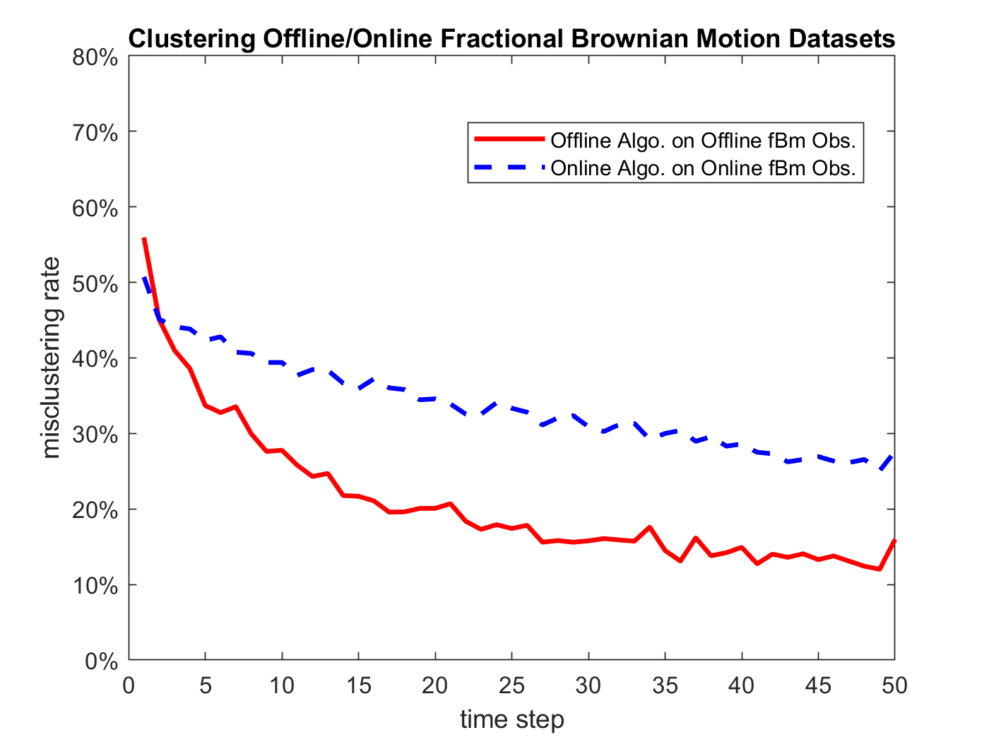
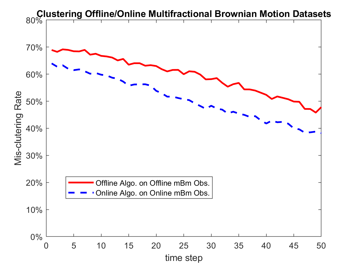
Figure 1: The top graph illustrates the mis-clustering rates of offline algorithm (Algorithm 1, solid red line), and online algorithm (Algorithm 2, dashed blue line) for fBm datasets. The bottom graph illustrates the mis-clustering rates of offline algorithm (Algorithm 1, solid red line), and online algorithm (Algorithm 2, dashed blue line) for mBm datasets.

References

- Aghabozorgi et al., (2015) Aghabozorgi, S., Shirkhorshidi, A. S., and Wah, T. Y. (2015). Time-series clustering - a decade review. Information Systems, 53:16–38.
- Ayache et al., (2000) Ayache, A., Cohen, S., and Lévy-Véhel, J. (2000). The covariance structure of multifractional Brownian motion, with application to long range dependence. In Acoustics, Speech, and Signal Processing, 2000. ICASSP’00. Proceedings. 2000 IEEE International Conference on, volume 6, pages 3810–3813. IEEE.
- Ayache and Lévy-Véhel, (2004) Ayache, A. and Lévy-Véhel, J. (2004). On the identification of the pointwise Hölder exponent of the generalized multifractional Brownian motion. Stochastic Processes and their Applications, 111(1):119–156.
- Boufoussi et al., (2008) Boufoussi, B., Dozzi, M., and Guerbaz, R. (2008). Path properties of a class of locally asymptotically self-similar processes. Electronic Journal of Probability, 13(29):898–921.
- Buard et al., (2010) Buard, B., Humeau, A., Rousseau, D., Chapeau-Blondeau, F., and Abrahamc, P. (2010). Pointwise Hölder exponents of a model for skin laser doppler flowmetry signals based on six nonlinear coupled oscillators with linear and parametric couplings: Comparison with experimental data from young healthy subjects. IRBM, 31:175–181.
- Damian et al., (2007) Damian, D., Orešič, M., and Verheij, E. e. a. (2007). Applications of a new subspace clustering algorithm (COSA) in medical systems biology. Metabolomics, 3(1):69–77.
- et al., (2018) et al., M. (2018). Clustering gene expression time series data using an infinite Gaussian process mixture model. PLoS Comput Biol, 14(1):e1005896.
- Falconer, (2002) Falconer, K. (2002). Tangent fields and the local structure of random fields. Journal of Theoretical Probability, 15(3):731–750.
- Höfling and Franosch, (2013) Höfling, F. and Franosch, T. (2013). Anomalous transport in the crowded world of biological cells. Reports on Progress in Physics, 76(4):046602.
- Humeau et al., (2007) Humeau, A., Chapeau-Blondeau, F., Rousseau, D., Tartas, M., Fromy, B., and Abraham, P. (2007). Multifractality in the peripheral cardiovascular system from pointwise Hölder exponents of laser doppler flowmetry signals. iophysical Journal, 93(12):L59–L61.
- Jääskinen et al., (2014) Jääskinen, V., Parkkinen, V., Cheng, L., and Corander, J. (2014). Bayesian clustering of DNA sequences using markov chains and a stochastic partition model. Stat. Appl. Genet. Mol. Biol., 13(1):105–121.
- Khaleghi and Ryabko, (2012) Khaleghi, A. and Ryabko, D. (2012). Locating changes in highly dependent data with unknown number of change points. In Advances in Neural Information Processing Systems, pages 3086–3094.
- Khaleghi and Ryabko, (2014) Khaleghi, A. and Ryabko, D. (2014). Asymptotically consistent estimation of the number of change points in highly dependent time series. In International Conference on Machine Learning, pages 539–547.
- Khaleghi et al., (2016) Khaleghi, A., Ryabko, D., Mari, J., and Preux, P. (2016). Consistent algorithms for clustering time series. Journal of Machine Learning Research, 17(3):1–32.
- Mandelbrot and van Ness, (1968) Mandelbrot, B. and van Ness, J. W. (1968). Fractional Brownian motions, fractional noises and applications. SIAM Review, 10(4):422–437.
- Marquez-Lago et al., (2012) Marquez-Lago, T. T., Leier, A., and Burrage, K. (2012). Anomalous diffusion and multifractional brownian motion: simulating molecular crowding and physical obstacles in systems biology. IET Systems Biology, 6(4):134–142.
- Maruyama, (1970) Maruyama, G. (1970). Infinitely divisible processes. Theory of Probability and its Applications, 15(1):1–22.
- Peltier and Véhel, (1995) Peltier, R.-F. and Véhel, J. L. (1995). Multifractional Brownian motion: definition and preliminary results. apport de recherche de l’INRIA, INRIA, no. 2645:239–265.
- Peng et al., (2018) Peng, Q., Rao, N., and Zhao, R. (2018). Clustering analysis on locally asymptotically self-similar processes with known number of clusters. arXiv, 1804.06234v1.
- Peng et al., (2019) Peng, Q., Rao, N., and Zhao, R. (2019). Covariance-based dissimilarity measures applied to clustering wide-sense stationary ergodic processes. Accepted by Machine Learning, arXiv, 1801.09049v4.
- S̀lezak, (2017) S̀lezak, J. (2017). Asymptotic behaviour of time averages for non-ergodic Gaussian processes. Annals of Physics, 383:285–311.
- Taqqu, (2013) Taqqu, M. S. (2013). Benoît Mandelbrot and fractional Brownian motion. Statistical Science, 28(1):131–134.
- Zhao et al., (2014) Zhao, W., Zou, W., and Chen, J. J. (2014). Topic modeling for cluster analysis of large biological and medical datasets. BMC Bioinformatics, 15:S11.