Solving Partial Differential Equations on Closed Surfaces
with Planar Cartesian Grids

Abstract

We present a general purpose method for solving partial differential equations on a closed surface, based on a technique for discretizing the surface introduced by Wenjun Ying and Wei–Cheng Wang [J. Comput. Phys. 252 (2013), pp. 606–-624] which uses projections on coordinate planes. Assuming it is given as a level set, the surface is represented by a set of points at which it intersects the intervals between grid points in a three-dimensional grid. They are designated as primary or secondary. Discrete functions on the surface have independent values at primary points, with values at secondary points determined by an equilibration process. Each primary point and its neighbors have projections to regular grid points in a coordinate plane where the equilibration is done and finite differences are computed. The solution of a p.d.e. can be reduced to standard methods on Cartesian grids in the coordinate planes, with the equilibration allowing seamless transition from one system to another. We observe second order accuracy in examples with a variety of equations, including surface diffusion determined by the Laplace-Beltrami operator and the shallow water equations on a sphere.

Subject Classification: 65M06, 65M50, 58J35, 58J45, 35Q86

Keywords: Cartesian grids, surface diffusion, Laplace-Beltrami operator, shallow water equations, closed surfaces, partial differential equations, finite difference methods

1 Introduction

We present a general purpose method for solving partial differential equations on a closed surface, based on a technique for discretizing the surface introduced by Wenjun Ying and Wei-Cheng Wang [32], which uses projections on coordinate planes. Assuming it is given as a level set, the surface is represented by a set of points at which it intersects the intervals between grid points in a three-dimensional grid. We will call these cut points. They are designated as primary or secondary. Discrete functions on the surface have independent values at primary points, and values at secondary points are determined from those by an equilibration process. Each primary point and its neighbors have projections to regular grid points in a coordinate plane where computations can be done, including the equilibration and calculation of finite differences. The solution of a p.d.e. can be reduced to standard methods on Cartesian grids in the coordinate planes, with the equilibration allowing seamless transition from one coordinate system to another. We observe second order accuracy in examples with a variety of equations.

To determine the primary points, we find the closest grid point to each cut point. Among those cut points which share the same closest grid point, we designate the one closest to the grid point as primary and any others as secondary. (See Figure 1.) This choice has the effect of determining which coordinate plane should be used. If, for example, a primary point has the form $(ih,jh,z(ih,jh))$, then the component of the normal vector in the $z$-direction is the largest in magnitude, within tolerance $O(h)$; see Lemma 2.1 below. Thus the surface has the form $z=z(x,y)$ near this primary point, and calculations are done on regular grid points in the $xy$-plane using projections of neighboring cut points on vertical grid intervals. However, some of these neighbors may be secondary points. The primary points are distributed quasi-uniformly; see Lemma 2.2. The procedure for selecting primary and secondary points and listing neighbors and coefficients for finite differences and equilibration is explained in the next section.

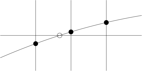
Figure 1: Primary (filled) and secondary (unfilled) cut points for a planar curve.

To solve partial differential equations on a surface using this approach we need to write the equations in each of three coordinate systems: (1) $(y,z)$, with $x=x(y,z)$; (2) $(z,x)$, with $y=y(z,x)$; and (3) $(x,y)$, with $z=z(x,y)$. To perform an explicit update in a time-dependent p.d.e., we update the unknown at each primary point in the appropriate coordinate system. We then equilibrate to obtain the updated values at the secondary points. The examples presented here illustrate how standard differential operators can be expressed in the coordinates, including the Laplace-Beltrami operator, the surface gradient and surface divergence. Only basic differential geometry is needed for this special choice of coordinates. We begin in Section 3 with a diffusion equation or a Poisson equation on a surface in which the differential operator is the Laplace-Beltrami operator. The discrete LB operator has a nine-point stencil in the coordinate plane. We discuss the spectrum and resolvent.

In Section 4 we apply this method to a linear advection equation and to the shallow water equations on a sphere. Formulas are obtained in the coordinate systems for transport by a tangential velocity field, surface gradient and divergence, and the material or substantial derivative, writing the tangential velocity as a three-vector. The formulas are not drastically different from those in the plane. We solve the equations for a standard test problem with a version of the Lax-Wendroff method. Nonlinear hyperbolic equations such as the shallow water equations are difficult to solve accurately and require more careful methods; here we have only the limited goal of establishing the feasibility of the present approach for such problems.

It is often desirable to monitor integrals of evolving quantities, such as conserved mass. In the present setting surface integrals can be computed in a natural way introduced in [31] and [2], using the cut points as quadrature points. This rule is summarized in Appendix B.

Often numerical methods for p.d.e.’s on surfaces use triangulation and finite elements [12]. Other methods use extension of the p.d.e. to a neighborhood of the surface [4, 23]. The closest point method [8, 19, 18, 20, 22] uses an extension such that e.g. the LB operator becomes the usual Laplacian; it can apply to point clouds and to moving surfaces. In [9] a variational principle on the surface is extended to a neighborhood and an extended p.d.e. is derived. The method of [16, 17, 28] is also suitable for point clouds; it uses a local coordinate grid near each point to find the surface and derivatives of the unknown using least squares. Radial basis functions have also been used to discretize the LB operator [24].

The shallow water equations are used as a depth-averaged model of global atmospheric motion. Because of their fundamental importance, a large amount of work has been devoted to their accurate solution using a variety of approaches. Reviews with emphasis on gridding include [25, 30]. An approach using Cartesian grids on the sphere was given in [26]. The velocity is treated as a three-vector in some work including [3, 14, 26]. Riemann solvers were used e.g. in [3, 7, 27]. Radial basis functions are also used [13].

The present method is quite simple and direct. Provided the surface is fairly smooth and known as a level set, the solution of a p.d.e. is performed with conventional finite differences on regular two-dimensional grids without boundary conditions. Variables do not need to be extended beyond the surface. In the applications given here, the projected problems are not very different from standard ones in the plane. It appears that familiar numerical methods in the plane can be used on surfaces when combined with this discretization. Possible further applications are discussed briefly in Section 5. However, this approach could not easily be adapted to a surface given as a point cloud, as in [17, 19, 28], or a surface with varying spatial scales, as in [17, 28]. The surface discretization used here was introduced in [32] in order to solve boundary value problems in the integral equation formulation, replacing the computation of boundary integrals with a finite difference method for equivalent interface problems.

Although some analysis given here supports the validity of these methods, it seems difficult to prove convergence. The equilibration appears to obstruct the use of standard arguments based on the maximum principle or summation by parts. We hope this challenge can be met in the future.

We describe the surface discretization in detail in Section 2. In Section 3 we formulate the discrete Laplace-Beltrami operator and apply it to a diffusion equation on various surfaces as well as the corresponding Poisson equation. We compute the lowest eigenvalues of the discrete LB operator on the sphere and present some partial information about the resolvent. In Section 4 we first solve a linear advection equation on a sphere with a known exact solution. We then express several differential operators in the coordinates and formulate the shallow water equations on a sphere. We compute the solution for a test problem from [29]. We conclude with some discussion in Section 5 of possible further work. In Appendix A it is proved that the discrete LB operator has positive resolvent for the special case of a curve in ${\mathbb{R}}^{2}$. The quadrature rule for surface integrals is given in Appendix B. Calculations were done in Matlab.

2 Surface discretization

We outline the procedure for discretizing the surface, give some details, and then explain the equilibration process. (Cf. [32], Sections 3–5.) We assume the surface has the form $\phi(x,y,z)=0$ with the level set function $\phi$ known at least at the grid points in ${\mathbb{R}}^{3}$. We assume $\phi$ is $C^{2}$ and $|\nabla\phi|\geq c_{0}$ on the surface for some $c_{0}>0$. The steps are these:

1. Choose a three-dimensional grid with size $h$ covering the surface. Label each grid point as inside or outside the surface according to the sign of $\phi$.

2. Find the grid intervals, e.g. from $(ih,jh,kh)$ to $(ih,jh,(k+1)h)$, with one grid point inside and one outside.

3. Find a cut point on the surface in each interval found in step 2, or in a restricted subset of intervals. Form sets of cut points $\Gamma_{\nu}$, $\nu=1,2,3$, where those in $\Gamma_{3}$ have the form $(ih,jh,z(ih,jh))$ etc.

4. Assign to each cut point the closest grid point.

5. For each grid point, designate the closest cut point assigned to it in step 4, if any, as primary and any others as secondary. Assign to each secondary point its associated primary point. (See Fig. 1 and [32], Figs. 2 and 3.)

6. For each primary point in $\Gamma_{\nu}$ list the neighboring cut points in $\Gamma_{\nu}$, some of which may be secondary. E.g., if $(ih,jh,z(ih,jh))\in\Gamma_{3}$, include $(i^{\prime}h,j^{\prime}h,z(i^{\prime}h,j^{\prime}h))$ with $|i^{\prime}-i|\leq 1$ and $|j^{\prime}-j|\leq 1$.

7. For each secondary point, find (at least) three points and coefficients needed for quadratic interpolation. The center point is the associated primary point, and the other two are its neighbors in the same set $\Gamma_{\nu}$. E.g., if $\bf s$ is a secondary point in $\Gamma_{1}$ with the form ${\bf s}=(x,jh,kh)$, with closest grid point $(ih,jh,kh)$, and $(ih,jh,z(ih,jh))\in\Gamma_{3}$ is the associated primary point, the two neighbors are $(ih\pm h,jh,z^{\pm})$. The coefficients are in (2.1) below.

In step 1, if a grid point happens to be on the surface, it can be assigned inside or outside. In step 3, we do not need to find all secondary points, as explained below. In step 3, if the cut point is a grid point, we need more information to determine which set $\Gamma_{\nu}$ it should belong to. We could do this by determining the largest component of the normal vector ${\bf n}=\pm\nabla\phi/|\nabla\phi|$ or simply match with a neighboring primary point which is not a grid point. In steps 4 and 5, in case of equal distances we can choose arbitrarily.

It is not necessary, and could be difficult, to find all secondary points. To avoid this, we can choose $\eta<1/\sqrt{3}$ and find only those cut points in $\Gamma_{\nu}$ such that $|n_{\nu}|\geq\eta$, where $n_{\nu}$ is the $\nu$-component of the unit normal to the surface. The cut points omitted in this way are not needed as neighbors of the primary points. We can reject these points by excluding intervals in step 2 for which $|n_{\nu}|<\eta$ at an endpoint. The admissible cut points are well separated: If $h$ is small enough, depending on the first two derivatives of the surface, a grid interval can have at most one admissible cut point. The admissible points can be found by a simple line search. These facts were shown in [31], pp. 11-18.

A discrete function on the surface will have independent values at the primary points, with values at the secondary points determined by those. We now explain the equilibration process that produces the values at the secondary points. Suppose as in step 7 that ${\bf s}\in\Gamma_{1}$ is a secondary point of the form ${\bf s}=(x,jh,kh)$, with closest grid point $(ih,jh,kh)$, so that $x=ih+\theta h$ with $|\theta|\leq{\textstyle\frac{1}{2}}$. If the associated primary point is ${\bf p}\in\Gamma_{3}$, then ${\bf p}=(ih,jh,z)$ for some $z$. The function value at ${\bf s}$ should agree with that interpolated from values at cut points ${\bf q^{\pm}}=(ih\pm h,jh,z^{\pm})\in\Gamma_{3}$ and $\bf p$. Given values $u({\bf p}),u({\bf q^{\pm}})$ we require $u({\bf s})$ to be the quadratic interpolation

$$u({\bf s})={\textstyle\frac{1}{2}}(-\theta+\theta^{2})u({\bf q^{-}})+(1-\theta^{2})u({\bf p})+{\textstyle\frac{1}{2}}(\theta+\theta^{2})u({\bf q^{+}})$$ (2.1)

However, since either or both of ${\bf q^{\pm}}$ may be secondary, we cannot simply interpolate secondary values from primary values. Instead, as in [32], Sec. 5.1, we solve a system of equations so that conditions such as (2.1) hold for all secondary points. The system of equations has the form

$$u^{s}=\Pi_{sp}u^{p}+\Pi_{ss}u^{s}$$ (2.2)

where $u^{s}$ and $u^{p}$ are column vectors of values on secondary and primary points, resp. and $\Pi_{sp}$, $\Pi_{ss}$ are matrices. The $i$th row of (2.2) gives the equation (2.1) for the $i$th secondary point. Each row of $\Pi_{ss}$ has at most two nonzero entries with absolute sum at most ${\textstyle\frac{1}{2}}(|\theta|+\theta^{2})+{\textstyle\frac{1}{2}}(|\theta|-\theta^{2})=|\theta|\leq{\textstyle\frac{1}{2}}$. Thus $I-\Pi_{ss}$ is strictly diagonally dominant and invertible. In particular equation (2.2) can be solved by the iteration

$$(u^{s})^{n+1}=\Pi_{sp}u^{p}+\Pi_{ss}(u^{s})^{n}$$ (2.3)

but in this work we invert the sparse matrix $I-\Pi_{ss}$, obtaining

$$u^{s}=(I-\Pi_{ss})^{-1}\Pi_{sp}u^{p}$$ (2.4)

The following two lemmas make precise the facts that the normal to the surface at a primary point in $\Gamma_{3}$ is largely in the $z$-direction, with $z=z(x,y)$ nearby on the surface, and the primary points are well distributed.

Lemma 2.1.

If ${\bf p}\in\Gamma_{3}$ is a primary point and the normal vector at $\bf p$ is $\bf n(p)$, then $|n_{\nu}({\bf p})|\leq(1+Ch)|n_{3}({\bf p})|$ for $\nu=1,2$, where $C$ depends on the first two derivatives of $\phi$. On the surface near ${\bf p}$, $z$ is a function of $(x,y)$ with $|z_{x}|,|z_{y}|\leq(1+Ch)$, and similarly for $\Gamma_{1}$, $\Gamma_{2}$.

Proof.

For convenience assume ${\bf p}=(0,0,\theta h)$ with $0<\theta\leq{\textstyle\frac{1}{2}}$. With $\nabla\phi=(\phi_{x},\phi_{y},\phi_{z})$, suppose $|\phi_{x}|\geq|\phi_{y}|$ at $\bf p$. Since $\bf{n(p)}=\pm\nabla\phi/|\nabla\phi|$, it will be enough to show that $|\phi_{x}|\leq(1+Ch)|\phi_{z}|$, with $C$ to be chosen. If this is not true, $|\phi_{x}|\geq|\nabla\phi|/\sqrt{3}$ and $|\phi_{z}|/|\phi_{x}|<(1+Ch)^{-1}$. Near $\bf p$, $x$ is a function of $z$ along the curve $\phi(x,0,z)=0$, with $x(\theta h)=0$ and $x^{\prime}(\theta h)=-\phi_{z}/\phi_{x}$ at $\bf p$. Also $x^{\prime\prime}$ is bounded, so that $|x^{\prime}(z)|\leq(1+Ch)^{-1}+C_{2}h$ near $\bf p$. We choose $C\geq 2C_{2}$ so that $|x^{\prime}(z)|<1$. Then $|x(\theta h)-x(0)|<\theta h$, or $|x(0)|<\theta h$, and thus $(x(0),0,0)$ is a cut point closer to $(0,0,0)$ than $\bf p$, contradicting the fact that $\bf p$ is primary. The second statement follows from the first and the equalities $z_{x}=-\phi_{x}/\phi_{z}$, $z_{y}=-\phi_{y}/\phi_{z}$. ∎

Lemma 2.2.

The set of primary points is quasi-uniform: Any two primary points are separated by distance at least $(\sqrt{2}/2)h-Ch^{2}$ with some constant $C$. For a primary point ${\bf p}=(ih,jh,z(ih,jh))\in\Gamma_{3}$, there is a primary point within distance $(3\sqrt{2}/2)h+Ch^{2}$ of $\bf p$ which belongs to the same grid point as the cut point ${\bf p^{+}}=((i+1)h,jh,z((i+1)h,jh))\in\Gamma_{3}$, and similarly for other neighbors of $\bf p$ and for $\Gamma_{1}$, $\Gamma_{2}$.

Proof.

Suppose ${\bf p}=(0,0,\theta h)$ is a primary point belonging to the grid point $(0,0,0)$, with $0\leq\theta\leq{\textstyle\frac{1}{2}}$. Any other point in $\Gamma_{3}$ is at least distance $h$ away. Any primary point $(x^{*},jh,kh)\in\Gamma_{1}$ is at distance at least $h$ provided $j\neq 0$ or $k\neq 0$ or $1$, and similarly for $\Gamma_{2}$. We are left to consider possible primary points of the form $(x^{*},0,0)$, $(x^{*},0,h)$, $(0,y^{*},0)$, or $(0,y^{*},h)$. In the first case, if $|x^{*}|<h/2$, a cut point $(x^{*},0,0)$ belongs to the grid point $(0,0,0)$ and must be secondary. Suppose $(x^{*},0,0)$ is a primary point with $|x^{*}|\geq h/2$. Then $|\phi_{z}|\leq(1+Ch)|\phi_{x}|$ as in Lemma 2.1. Also, because $\bf p$ is primary, $z$ is a function of $x$ on the curve $\phi(x,0,z)=0$, with $z^{\prime}=-\phi_{x}/\phi_{z}$, so that $|z^{\prime}|\geq 1-C_{1}h$. With $z(0)=\theta h$ and $z(x^{*})=0$, we have $|\theta h-0|\geq(1-C_{1}h)|x^{*}|$. Then $|(0,0,\theta h)-(x^{*},0,0)|\geq|x^{*}|(1+(1-C_{1}h)^{2})^{1/2}\geq(h/2)(\sqrt{2}-C_{2}h)$, with some $C_{2}$, and this is equivalent to the conclusion stated. For a cut point $(x^{*},0,h)$ we can argue similarly, using the bound $|z_{x}|\leq(1+Ch)$ and the fact that $h-\theta h\geq h/2$. Other cases are analogous to these.

For the second statement, we have $z=z(x,y)$ on the surface with $|z_{x}|\leq(1+Ch)$ as before, so that ${|\bf p^{+}-p|}\leq(\sqrt{2}+C^{\prime}h)\,h$. If ${\bf p^{+}}$ is secondary, the primary point belonging to the same grid point is within distance $(\sqrt{2}/2)h$ of $\bf p^{+}$, and the conclusion follows. ∎

3 The Laplace-Beltrami operator and diffusion equations

The discrete Laplace-Beltrami operator. The Laplace-Beltrami operator, or surface Laplacian, is the generalization of the usual Laplacian to a surface or manifold. For the unit sphere it is the angular part of the Laplacian. It is invariant under change of coordinates and is expressed in any coordinate system in terms of the metric tensor. Suppose $(\xi_{1},\xi_{2})$ are coordinates on a surface $\Gamma\subseteq{\mathbb{R}}^{3}$ so that part of $\Gamma$ is given as ${\bf X}(\xi_{1},\xi_{2})$. At each point we have tangent vectors ${\bf X}_{i}=\partial{\bf X}/\partial\xi_{i}$, $i=1,2$, metric tensor $g_{ij}={\bf X_{i}}\cdot{\bf X_{j}}$, the inverse $g^{ij}=(g_{ij})^{-1}$, and $g=\det{g_{ij}}$. The Laplace-Beltrami operator applied to a scalar function $u$ on $\Gamma$ is

$$\Delta u\,=\,\frac{1}{\sqrt{g}}\sum_{i,j=1}^{2}\frac{\partial}{\partial\xi_{i}}\left(\sqrt{g}g^{ij}\frac{\partial u}{\partial\xi_{j}}\right)$$ (3.1)

We can discretize the LB operator in divergence form on a regular grid using a stencil with 9 points. We will describe the discrete operator $\Delta_{h}$, with grid size $h$, at a point labeled $(\xi_{1},\xi_{2})=(0,0)$ for convenience, using points $(\sigma_{1}h,\sigma_{2}h)$ with $\sigma_{1},\sigma_{2}=-1,0,1$. We will set $a^{ij}=\sqrt{g}g^{ij}$ and use notation such as

$$a^{ij}_{+-}=(a^{ij}(h,-h)+a^{ij}(0,0))/2$$

Because of the mixed derivatives, we begin with the second difference along a diagonal,

$$L_{\diagup}(a^{12},u)\,=\,\left(a^{12}_{++}(u(h,h)-u(0,0))-a^{12}_{--}(u(0,0)-u(-h,-h))\right)/h^{2}$$ (3.2)

To approximate (3.2) we use the Taylor expansion

$$a^{12}_{++}\,=\,a^{12}+h(a^{12}_{1}+a^{12}_{2})/2+h^{2}(a^{12}_{11}+a^{12}_{22}+2a^{12}_{12})/4+O(h^{3})$$ (3.3)

and the corresponding formula for $a^{12}_{--}$, where the quantities on the right are evaluated at $(0,0)$ and subscripts denote derivatives. We find

$$\left(a^{12}_{++}+a^{12}_{--}\right)/2=a^{12}+O(h^{2})\,,\qquad\left(a^{12}_{++}-a^{12}_{--}\right)=h(a^{12}_{1}+a^{12}_{2})+O(h^{3})$$ (3.4)

Similarly we have

$$u(\pm h,\pm h)\,=\,u\;\pm\;h(u_{1}+u_{2})+h^{2}(u_{11}+u_{22}+2u_{12})/2\pm c_{3}\,h^{3}+O(h^{4})$$ (3.5)

from which we get

$$u(h,h)+u(-h,-h)-2u(0,0)=h^{2}(u_{11}+u_{22}+2u_{12})+O(h^{4})\,,\\ u(h,h)-u(-h,-h)=2h(u_{1}+u_{2})+O(h^{3})$$ (3.6)

We rearrange (3.2) and use (3.4) and (3.6) to obtain

$$L_{\diagup}(a^{12},u)=\left(a^{12}_{++}+a^{12}_{--}\right)(u(h,h)+u(-h,-h)-2u(0,0))/2h^{2}\\ +\left(a^{12}_{++}-a^{12}_{--}\right)(u(h,h)-u(-h,-h))/2h^{2}\\ \,=\,a^{12}(u_{11}+u_{22}+2u_{12})\,+\,(a^{12}_{1}+a^{12}_{2})(u_{1}+u_{2})+O(h^{2})$$ (3.7)

We also use the standard second differences in direction $i=1$ or $2$

$$L_{1}({\tilde{a}}^{11},u)\,=\,\left({\tilde{a}}^{11}_{+0}(u(h,0)-u(0,0))-{\tilde{a}}^{11}_{-0}(u(0,0)-u(-h,0))\right)/h^{2}$$ (3.8)

$$L_{2}({\tilde{a}}^{22},u)\,=\,\left({\tilde{a}}^{22}_{0+}(u(0,h)-u(0,0))-{\tilde{a}}^{22}_{0-}(u(0,0)-u(0,-h))\right)/h^{2}$$ (3.9)

with ${\tilde{a}}^{ii}=a^{ii}-a^{12}$. As above we find

$$L_{i}(a^{ii}-a^{12},u)\,=\,(a^{ii}-a^{12})u_{ii}\,+\,(a^{ii}_{i}-a^{12}_{i})u_{i}\,+\,O(h^{2})$$ (3.10)

We now define

$$\Delta_{h}u\,\equiv\,\left(L_{1}(a^{11}-a^{12},u)+L_{2}(a^{22}-a^{12},u)\,+\,L_{\diagup}(a^{12},u)\right)/\sqrt{g}$$ (3.11)

From (3.7),(3.10) we have, after combining terms,

$$\sqrt{g}\,\Delta_{h}u\,=\,a^{11}u_{11}+a^{22}u_{22}+2a^{12}u_{12}\\ +a^{11}_{1}u_{1}+a^{22}_{2}u_{2}+a^{12}_{1}u_{2}+a^{12}_{2}u_{1}+O(h^{2})\\ \,=\,(a^{11}u_{1})_{1}+(a^{22}u_{2})_{2}+(a^{12}u_{1})_{2}+(a^{12}u_{2})_{1}+O(h^{2})$$ (3.12)

Comparing with (3.1), we see that $\Delta_{h}u=\Delta u+O(h^{2})$, as for usual centered second difference operators.

We could alternatively use the other diagonal and define

$$L_{\diagdown}(a^{12},u)\,=\,\left(a^{12}_{-+}(u(-h,h)-u(0,0))-a^{12}_{+-}(u(0,0)-u(h,-h))\right)/h^{2}$$ (3.13)

We find as above that

$$L_{\diagdown}(a^{12},u)\,=\,a^{12}(u_{11}+u_{22}-2u_{12})\,+\,(-a^{12}_{1}+a^{12}_{2})(-u_{1}+u_{2})+O(h^{2})$$ (3.14)

Proceeding as before we define

$$\Delta_{h}u\,\equiv\,\left(L_{1}(a^{11}+a^{12},u)+L_{2}(a^{22}+a^{12},u)\,-\,L_{\diagdown}(a^{12},u)\right)/\sqrt{g}$$ (3.15)

It is again accurate to $O(h^{2})$. We use (3.11) if $g^{12}\geq 0$ and (3.15) if $g^{12}\leq 0$.

In this work the coordinates are always $(y,z)$, $(z,x)$, or $(x,y)$, where ${\bf X}=(x,y,z)$. In the third case, for example, $z=z(x,y)$ and

$$g=1+z_{x}^{2}+z_{y}^{2}\,,\quad g^{11}=(1+z_{y}^{2})/g\,,\quad g^{12}=-z_{x}z_{y}/g\,,\quad g^{22}=(1+z_{x}^{2})/g$$ (3.16)

For points in $\Gamma_{3}$ we have $|z_{x}|,|z_{y}|\leq 1+O(h)$, according to Lemma 2.1. It follows that $g^{ii}-|g^{12}|>0$, and the off-diagonal coefficients in (3.11),(3.15) are $\geq 0$ while the coefficient of $u(0,0)$ is $<0$, assuming $g^{12}\geq 0$ or $g^{12}\leq 0$ respectively.

For a familiar surface, such as the sphere of radius $r$, we may prefer to replace (3.11),(3.15) with a non-divergence form,

$$\Delta_{h}u\,=\,(g^{11}-g^{12})D^{2}_{1}u\,+\,(g^{22}-g^{12})D^{2}_{2}u\,+\,g^{12}D^{2}_{\diagup}u\,+\,b_{1}D_{1}u+b_{2}D_{2}u$$ (3.17)

$$\Delta_{h}u\,=\,(g^{11}+g^{12})D^{2}_{1}u\,+\,(g^{22}+g^{12})D^{2}_{2}u\,-\,g^{12}D^{2}_{\diagdown}u\,+\,b_{1}D_{1}u+b_{2}D_{2}u$$ (3.18)

where $D^{2}_{\diagup}u=L_{\diagup}(1,u)$ etc., with centered differences in the last two terms. For the sphere with $z=z(x,y)$,

$$g=r^{2}/z^{2}\,,\quad g^{11}=(r^{2}-x^{2})/r^{2}\,,\quad g^{22}=(r^{2}-y^{2})/r^{2}\,,\quad g^{12}=-xy/r^{2}\,,$$ (3.19)

$$b_{1}=-2x/r^{2}\,,\quad b_{2}=-2y/r^{2}$$ (3.20)

The diffusion equation. The prototype equation for diffusion on a surface $\Gamma$ is

$$u_{t}\,=\,\alpha\Delta u\quad\mbox{on\;}\Gamma$$ (3.21)

where $u(\cdot,t)$ is function on $\Gamma$, $\Delta$ is the Laplace-Beltrami operator and $\alpha$ is a coefficient. To solve this equation with a specified initial state we discretize the surface as in Section 2 and replace $u$ with a function $u_{h}$ on $\Gamma_{h}$, the set of cut points, both primary and secondary. We also use the restriction $u^{p}_{h}$ to the set of primary points $\Gamma^{p}_{h}$. We think of both as column vectors. We calculate the discrete LB operator $\Delta_{h}$ applied to $u_{h}$ at points in $\Gamma^{p}_{h}$. Thus $\Delta_{h}$ is an $n_{p}\times n_{tot}$ matrix where $n_{p}$ is the number of primary points and $n_{tot}$ is the number of all admissible points, primary and secondary. The values of $\Delta_{h}u_{h}$ at primary points are found using either (3.11),(3.15) or (3.17),(3.18) in the three coordinate systems. We can extend any function $f^{p}_{h}$ on $\Gamma^{p}_{h}$ to the remaining secondary points in $\Gamma_{h}$ by the equilibration $E_{h}$ defined in (2.4), i.e.,

$$E_{h}f^{p}_{h}\,=\,(f^{p}_{h}\;f^{s}_{h})^{T}\,,\qquad f^{s}_{h}\,=\,(I-\Pi_{ss})^{-1}\Pi_{sp}f^{p}_{h}$$ (3.22)

so that $E_{h}$ is an $n_{tot}\times n_{p}$ matrix.

To solve (3.21) we replace $\Delta u$ by $E_{h}\Delta_{h}u_{h}$ and select a time stepping method. We have used the forward Euler method and BDF2, the second order backward difference formula, as representatives of explicit and implicit methods. With time step $k$, the forward Euler method approximates (3.21) with

$$u^{n+1}_{h}\,=\,u^{n}_{h}+k\alpha E_{h}\Delta_{h}u^{n}_{h}$$ (3.23)

whereas for BDF2 we have

$$u^{n+1}_{h}\,=\,(I-\frac{2}{3}k\alpha E_{h}\Delta_{h})^{-1}(\frac{4}{3}u^{n}_{h}-\frac{1}{3}u^{n-1}_{h})$$ (3.24)

We have not proved that the inverse matrix in (3.24) exists, but we obtain it in our computations. Properties of this resolvent matrix are discussed further below. We could instead formulate the solution in terms of $u^{p}_{h}$ on $\Gamma^{p}_{h}$. The forward Euler version in this case would be

$$u^{p,n+1}_{h}\,=\,u^{p,n}_{h}+k\alpha\Delta_{h}E_{h}u^{p,n}_{h}$$ (3.25)

Assuming the initial state is equilibrated, then (3.23) and (3.25) are equivalent, i.e., if $u^{p,n}_{h}$ solves (3.25) then $u^{n}_{h}=E_{h}u^{p,n}_{h}$ solves (3.23). Similarly, we find that if $f_{h}$ on $\Gamma_{h}$ is equilibrated, with $f_{h}=E_{h}f^{p}_{h}$, and if $v^{p}_{h}$ on $\Gamma^{p}_{h}$ satisfies $(I-\kappa\Delta_{h}E_{h})v^{p}_{h}=f^{p}_{h}$, then $v_{h}=E_{h}v^{p}_{h}$ on $\Gamma_{h}$ satisfies $(I-\kappa E_{h}\Delta_{h})v_{h}=f_{h}$. Thus the resolvents of the $n_{tot}\times n_{tot}$ matrix $E_{h}\Delta_{h}$ and the $n_{p}\times n_{p}$ matrix $\Delta_{h}E_{h}$ are closely related. We study the latter operator further below.

As a first example for the diffusion equation we choose $\Gamma$ to be the unit sphere and the initial state to be a spherical harmonic, as in several references. We take

$$u^{0}(x,y,z)=7(x-2y)(15z^{2}-3)/8$$ (3.26)

Then $\Delta u^{0}=-12u^{0}$ on the unit sphere. We choose $\alpha=1/12$ in (3.21) so that the exact solution is $u=e^{-t}u^{0}$. We embed the sphere in a computational box $[-1.2,1.2]^{3}$ and introduce a grid with $N$ intervals in each direction, so that $h=2.4/N$. We discretize as in Section 2. The parameter $\eta$ is $.45$. We then solve to time $t=1$ with either the forward Euler method (FE) or BDF2, started with a backward Euler step. We use either the divergence form of $\Delta_{h}$ in (3.11),(3.15) or the nondivergence form (3.17),(3.18). For each $N$ we choose time step $k=8/N^{2}$ with FE and $k=1/(2N)$ with BDF2. Relative errors in the four cases are shown in Table 3.1. The relative $L^{2}$ error is

$$\|u^{comp}-u^{exact}\|/\|u^{exact}\|\,,\qquad\|w\|^{2}=(1/n_{tot})\sum_{{\bf X}\in\Gamma_{h}}w({\bf X})^{2}$$ (3.27)

The relative maximum error is a similar ratio of absolute maxima. We see that the convergence is about second order in each case. The errors are somewhat larger for the divergence form, but it can be used for a general surface.

Table 3.1: Relative errors for diffusion on the unit sphere

	FE		BDF2		FE		BDF2
	nondiv		nondiv		div		div
N	max	$L^{2}$	max	$L^{2}$	max	$L^{2}$	max	$L^{2}$
80	4.94e-4	3.21e-4	8.24e-4	4.64e-4	1.01e-3	8.65e-4	1.45e-3	1.45e-3
160	1.03e-4	5.92e-5	1.90e-4	1.32e-4	2.44e-4	2.27e-4	3.67e-4	3.77e-4
320	1.96e-5	1.67e-5	2.21e-5	2.44e-5	4.96e-5	5.46e-5	8.65e-5	9.04e-5
640	5.03e-6	4.41e-6	4.53e-6	4.53e-6	1.19e-5	1.35e-5	2.04e-5	2.05e-5

For our next examples we use two different surfaces. The first is the ellipsoid

$$x^{2}/a^{2}\,+\,y^{2}/b^{2}\,+\,z^{2}/c^{2}\,=\,1$$ (3.28)

with $a=1$, $b=.8$ and $c=.65$. The second is obtained by rotating a Cassini oval about the $z$-axis,

$$(x^{2}+y^{2}+z^{2}+a^{2})^{2}\,-\,4a^{2}(x^{2}+y^{2})\,=\,b^{4}$$ (3.29)

with $a=.65$ and $b/a=1.1$, a nonconvex surface. In both cases we solve (3.21) with $\alpha=.1$ and initial state $u^{0}(x,y,z)=\cos(x-y+z)$. We compute $\Delta_{h}$ as in (3.11), (3.15). We use FE with $k=8/N^{2}$ and BDF2 with $k=1/(10N)$ and solve to time $t=1$. Since we do not know the exact solution, we measure errors by comparing successive runs. With $N=80$, $160$, $320$, we compute successive $L^{2}$ errors $\varepsilon_{N}=\|u^{N}-u^{2N}\|$, with norm as in (3.27); similarly we find successive maximum errors. Both are displayed in Table 3.2. The convergence for the ellipsoid is about second order. For the Cassini oval the rate is less clear, but the decrease from $N=80$ to $N=320$ is more rapid than second order.

Table 3.2: Successive errors for diffusion on two surfaces

	Ellipsoid				Cassini Oval
	FE		BDF2		FE		BDF2
N	max	$L^{2}$	max	$L^{2}$	max	$L^{2}$	max	$L^{2}$
80	2.35e-4	6.32e-5	2.53e-4	9.46e-5	6.68e-4	1.68e-4	6.52e-4	1.88e-4
160	6.47e-5	1.73e-5	7.15e-5	2.47e-5	9.09e-5	3.10e-5	9.07e-5	3.39e-5
320	1.56e-5	4.60e-6	2.06e-5	6.81e-6	2.72e-5	9.12e-6	2.33-5	9.76-6

Spectrum and resolvent of the discrete LB operator. We will call the $n_{p}\times n_{p}$ matrix $\Delta^{red}_{h}=\Delta_{h}E_{h}$ the reduced LB operator. It approximates the LB operator discretized to the primary points. To compare it to the exact operator, we compute its lowest eigenvalues on the unit sphere. The exact spherical Laplacian has eigenvalues $\lambda_{n}=-n(n+1)$, $n\geq 0$, with multiplicity $2n+1$. Table 3.3 gives the errors in the first 49 eigenvalues for $\Delta^{red}_{h}$ for various $N$. For $1\leq n\leq 7$, the maximum absolute error is displayed for the $2n+1$ eigenvalues close to $\lambda_{n}$. They appear to converge to second order, with larger errors for higher $n$. Here $\Delta^{red}_{h}$ was computed in divergence form. The nondivergence form gives somewhat smaller errors, except for $n=1$. Eigenvalues were also computed in [17].

Table 3.3: Absolute errors in eigenvalues for the spherical Laplacian

$-\lambda$	mult	40	80	160	320
0	1	2.2e-15	3.1e-14	1.2e-14	1.8e-14
2	3	3.01e-3	7.64e-4	1.10e-4	3.77e-5
6	5	3.19e-2	7.97e-3	1.99e-3	4.95e-4
12	7	6.93e-2	1.70e-2	3.82e-3	1.02e-3
20	9	1.87e-1	4.67e-2	1.17e-2	2.91e-3
30	11	3.37e-1	8.45e-2	2.07e-2	5.25e-3
42	13	7.16e-1	1.79e-1	4.49e-2	1.13e-2

As noted in [17] it is desirable for a discretization of $I-k\Delta$ to be an M-matrix. A square matrix $A$ is called an M-matrix if the diagonal entries are $>0$, the off-diagonal entries are $\leq 0$, and $A$ is strictly diagonally dominant. It follows that $A^{-1}$ is positive, i.e., each entry of $A^{-1}$ is $\geq 0$. (E.g. see [15].) These properties have important consequences for the stability of schemes for elliptic and parabolic equations. For example, if $\Delta_{h}^{0}$ is the usual five-point Laplacian on a rectangle in ${\mathbb{R}}^{2}$ with periodic boundary conditions, $I-k\Delta_{h}^{0}$ is an M-matrix for $k>0$. The row sums of $(I-k\Delta_{h}^{0})^{-1}$ are $1$, since those of $\Delta_{h}^{0}$ are $0$. This fact and the positivity imply that the resolvent operator $(I-k\Delta_{h}^{0})^{-1}$, acting on vectors in maximum norm, has norm $1$. Consequently if the heat equation $u_{t}=\Delta_{h}^{0}u$ is solved with backward Euler time steps, the maximum of the solution is nonincreasing in time.

Our discrete LB operator $\Delta_{h}$, constructed as (3.11),(3.15), has the correct sign conditions, but the interpolation (2.1) has both signs. For this reason, $I-k\Delta_{h}^{red}$ fails to be an M-matrix in general. Nonetheless, we see in our computations that $(I-k\Delta_{h}^{red})^{-1}$ often has nonnegative entries. Constants are null vectors for $\Delta^{red}_{h}$, since a constant on the primary points equilibrates to the constant, and $\Delta_{h}$ applied to a constant vector gives zero. Thus the row sums of $\Delta^{red}_{h}$ are zero, and $(I-k\Delta_{h}^{red})^{-1}$ has row sums one. If $(I-k\Delta_{h}^{red})^{-1}\geq 0$ then it has norm $1$ as in the familiar case above. We observe that $(I-k\Delta_{h}^{red})^{-1}\geq 0$ for $k/h^{2}$ larger than $1$ but not for $k/h^{2}$ small. We are not able to prove this positivity for surfaces in ${\mathbb{R}}^{3}$, but we give a proof for closed curves in ${\mathbb{R}}^{2}$ in Appendix A, since it gives some insight into the interaction between the discrete LB operator and the equilibration. There are only a few results concerning properties of matrices perturbed from $M$-matrices, e.g. [5, 6].

The Poisson equation. For the exact LB operator, the Poisson equation

$$\Delta u\,=\,f\;\mbox{on\;}\Gamma$$ (3.30)

has a solution if and only if $\int f\,dS=0$, and the solution is unique up to an arbitrary constant (e.g. see [12]). We noted that for the reduced discrete operator $\Delta^{red}_{h}$ constants are null vectors. The eigenvalue computation for $\Delta_{h}^{red}$ suggests they are the only null vectors, so that the range has codimension one and solutions of the discrete equation are again unique except for a constant. We can attempt to solve the equation (3.30), given $f$ in the range, by augmenting the discrete problem to

$$\Delta_{h}^{red}u^{h}\,+\,\beta{\bf 1}\,=\,f^{h}\,,\qquad\sum u^{h}=0$$ (3.31)

where $f^{h}$ is the restriction to primary points, $\beta$ is an extra (scalar) unknown, ${\bf 1}$ is a vector of $1$’s, and the sum is over $\Gamma_{h}^{p}$. The extra term adjusts $f^{h}$ so that $f^{h}-\beta{\bf 1}$ can be in the range of $\Delta_{h}^{red}$. We expect that $f^{h}$ is close to being in the range of $\Delta_{h}^{red}$ and consequently $\beta$ will be small. Then $u^{h}$ should approximate the solution of (3.30) with $\Sigma u=0$. (Such a method was outlined in [15], Sec. 4.7 for the Neumann problem.)

We test this approach to solving (3.30) with a known exact solution. We define $u=\cos(x/r+y/r-2z/r)$ on ${\mathbb{R}}^{3}$, with $r^{2}=x^{2}+y^{2}+z^{2}$ and find the usual Laplacian $f$. Then the LB operator applied to $u$ on the unit sphere will equal $f$. We solve (3.31) on the unit sphere with this choice of $f$. We compare the computed solution with $u-u_{0}$ where $u$ is the exact solution and $u_{0}=n_{p}^{-1}\Sigma u$. (Note that $u_{0}$ depends on $h$.) With $N=80$, $160$, $320$, $640$ we find absolute maximum errors $9.20e\!-\!4$, $2.35e\!-\!4$, $5.70e\!-\!5$, $1.40e\!-\!5$, showing $O(h^{2})$ convergence.

4 Advection and flow on the sphere

A linear advection equation. As a test problem for transport on a surface, we have constructed a linear advection equation on the unit sphere with an exact solution. We will use $\varphi$ and $\theta$ for longitude and latitude, resp., with $0\leq\varphi\leq 2\pi\,$, $-\pi/2\leq\theta\leq\pi/2$, so that

$$x=\cos{\varphi}\cos{\theta}\,,\quad y=\sin{\varphi}\cos{\theta}\,,\quad z=\sin{\theta}$$ (4.1)

We set

$$r^{2}\,=\,\cos^{2}{\theta}\,=\,x^{2}+y^{2}\,=\,1-z^{2}$$ (4.2)

Our advection equation for unknown $\Phi(\varphi,\theta,t)$ is

$$\frac{\partial\Phi}{\partial t}\,+\,\frac{\partial\Phi}{\partial\varphi}\,-\,\cos{\varphi}\cos^{2}{\theta}\frac{\partial\Phi}{\partial\theta}\,=\,0$$ (4.3)

The vector field represents rotation about the vertical axis with oscillation in latitude. The equation can be solved by the method of characteristics. As initial state we take

$$\Phi(\varphi,\theta,0)\,=\,\cos^{2}{\theta}\,=\,r^{2}$$ (4.4)

The exact solution in rectangular coordinates is

$$\Phi=\frac{r^{2}}{\left(z+y(1-\cos{t})+x\sin{t}\right)^{2}+r^{2}}$$ (4.5)

To solve the initial value problem with the present method we first rewrite the p.d.e. (4.3) in each of the three coordinate systems, e.g. with $\Phi=\Phi(x,y)$ in $\Gamma_{3}$. The three forms are

$$\Phi_{t}+(x+xyz)\Phi_{y}-xr^{2}\Phi_{z}\,=\,0\,,\qquad x=x(y,z)$$ (4.6)

$$\Phi_{t}-xr^{2}\Phi_{z}+(x^{2}z-y)\Phi_{x}\,=\,0\,,\qquad y=y(z,x)$$ (4.7)

$$\Phi_{t}+(x^{2}z-y)\Phi_{x}+(x+xyz)\Phi_{y}\,=\,0\,,\qquad z=z(x,y)$$ (4.8)

We discretize the three equations using the MacCormack two-step version of the Lax-Wendroff method. With time step $k$, given $\Phi^{n}\approx\Phi(\cdot,nk)$ at all points, primary and secondary, the first step is to compute the update to $\Phi^{n}$ at primary points, equilibrate the update to secondary points, and add the update to $\Phi^{n}$ to obtain the predictor $\Phi^{*}$. Thus e.g. in the third system we compute the update at primary points

$$F^{*}\,=\,\,-\,(x^{2}z-y)D_{x}^{+}\Phi^{n}\,-\,(x+xyz)D_{y}^{+}\Phi^{n}$$ (4.9)

where $D_{x}^{+}$, $D_{y}^{+}$ are usual forward differences. After doing the same in all three systems, we equilibrate as in (2.4) to extend $F^{*}$ from primary points to $E_{h}F^{*}$ defined on all points, with $E_{h}$ as in (3.22). We then set

$$\Phi^{*}\,=\,\Phi^{n}\,+\,kE_{h}F^{*}$$ (4.10)

The second step uses a similar procedure with backward differences, with the update in the third system at the primary points

$$F^{n+1}=\,-\,(x^{2}z-y)D_{x}^{-}\Phi^{*}\,-\,(x+xyz)D_{y}^{-}\Phi^{*}$$ (4.11)

and after finding $F^{n+1}$ at primary points in all three systems

$$\Phi^{n+1}\,=\,\frac{1}{2}(\Phi^{n}+\Phi^{*})\,+\,\frac{k}{2}E_{h}F^{n+1}$$ (4.12)

We use grid size $h=2.4/N$ and time step $k=1/2N$ for various choices of $N$. Relative errors are displayed in Table 4.1. They are clearly $O(h^{2})$. The $L^{2}$ error is

$$\frac{\left(\sum\left|\Phi^{comp}({\bf p})-\Phi^{exact}({\bf p})\right|^{2}\right)^{1/2}}{\left(\sum|\Phi^{exact}({\bf p})|^{2}\right)^{1/2}}$$ (4.13)

where the sum is over all primary points and admissible secondary points. Similarly the relative maximum error is $\max|\Phi^{comp}-\Phi^{exact}|/\max|\Phi^{exact}|$. We also compute the surface integral of $\Phi$ using the method explained in Appendix B and display the relative error. (The integral is not constant in time since ${\bf v}$ does not have divergence zero.)

Table 4.1: Relative errors for the linear advection equation

N	time	max error	$L^{2}$ error	error in $\int\Phi$
80	1	3.29e-3	8.13e-4	1.47e-4
	2	7.12e-3	2.50e-3	1.70e-4
	5	3.32e-2	1.59e-2	-2.26e-3
160	1	7.59e-4	2.01e-4	3.63e-5
	2	1.76e-3	6.24e-4	4.19e-5
	5	8.32e-3	4.03e-3	-5.69e-4
320	1	1.79e-4	5.01e-5	9.12e-6
	2	4.37e-4	1.57e-4	1.04e-5
	5	2.13e-3	1.01e-3	-1.43e-4
640	1	4.43e-5	1.26e-5	2.28e-6
	2	1.10e-4	3.92e-5	2.64e-6
	5	5.34e-4	2.53e-4	-3.59e-5

Differential operators on a surface. Before proceeding it will be helpful to interpret this example in a setting independent of coordinates and discuss the surface gradient and divergence. The p.d.e. (4.3) in spherical coordinates is equivalent to

$$\frac{\partial\Phi}{\partial t}\,+\,{\bf v}\cdot\nabla\Phi\,=\,0$$ (4.14)

where $\nabla\Phi$ is the surface gradient and $\bf v$ is the tangential vector field

$${\bf v}\,=\,{\bf X}_{\varphi}-\cos{\varphi}\cos^{2}{\theta}{\bf X}_{\theta}\,=\,(x^{2}z-y,x+xyz,-xr^{2})^{T}$$ (4.15)

Here ${\bf X}=(x,y,z)$ and ${\bf X}_{\varphi}=\partial{\bf X}/\partial\varphi$ and ${\bf X}_{\theta}=\partial{\bf X}/\partial\theta$ are tangent vectors.

In general, if $(\xi_{1},\xi_{2})$ are coordinates on a surface, the tangent vectors ${\bf X}_{i}=\partial{\bf X}/\partial\xi_{i}$, $i=1,2$ form a basis of the tangent space at each point on the surface. With metric tensor $g_{ij}={\bf X}_{i}\cdot{\bf X}_{j}$ and inverse $g^{ij}=(g_{ij})^{-1}$, we have dual tangent vectors ${\bf X}^{*}_{i}=\Sigma_{j}g^{ij}{\bf X}_{j}$ so that ${\bf X^{*}_{i}}\cdot{\bf X_{j}}=\delta_{ij}$. For a scalar function $\Phi$ the surface gradient is

$$\nabla\Phi\,=\,\frac{\partial\Phi}{\partial\xi_{1}}{\bf X^{*}_{1}}\,+\,\frac{\partial\Phi}{\partial\xi_{2}}{\bf X^{*}_{2}}$$ (4.16)

Note that ${\bf X}_{i}\cdot\nabla\Phi=\partial\Phi/\partial\xi_{i}$. In the specific case $(\xi_{1},\xi_{2})=(x,y)$, with $z=z(x,y)$, we have ${\bf X}_{1}=(1,0,z_{x})^{T}$ and ${\bf X}_{2}=(0,1,z_{y})^{T}$. For a tangential vector field ${\bf v}=(v_{1},v_{2},v_{3})^{T}$ in Cartesian form as above, we have

$${\bf v}=v_{1}{\bf X}_{1}+v_{2}{\bf X}_{2}$$ (4.17)

so that

$${\bf v}\cdot\nabla\Phi=v_{1}\Phi_{x}+v_{2}\Phi_{y}$$ (4.18)

leading to the third form of the p.d.e. (4.8) above, and the other two are similar. For later use we note that, with $z=z(x,y)$, the surface gradient is

$$\nabla\Phi\,=\,(\Phi_{x},\Phi_{y},0)^{tan}$$ (4.19)

where $tan$ denotes the tangential part of the vector,

$${\bf w}^{tan}\,=\,{\bf w}\,-\,({\bf w}\cdot{\bf n}){\bf n}$$ (4.20)

as can be seen by checking the scalar product with ${\bf X}_{i}$.

The surface divergence of a tangential vector field in general coordinates on a surface is

$$\nabla\cdot{\bf v}\,=\,\frac{\partial{\bf v}}{\partial\xi_{1}}\cdot{\bf X^{*}_{1}}\,+\,\frac{\partial{\bf v}}{\partial\xi_{2}}\cdot{\bf X^{*}_{2}}$$ (4.21)

This is equivalent to a standard formula, e.g. in [1], $\nabla\cdot{\bf v}=g^{-1/2}\Sigma_{i}\partial(g^{1/2}v_{i})/\partial\xi_{i}$ with $v_{i}$ as in (4.17). For the unit sphere, again with coordinates $(x,y)$ and $z=z(x,y)$, a calculation gives

$$\nabla\cdot{\bf v}\,=\,v_{1,x}+v_{2,y}+(x/z^{2})v_{1}+(y/z^{2})v_{2}$$ (4.22)

Corresponding remarks apply to the other coordinate systems, $(x,y)$ or $(z,x)$.

The shallow water equations. The shallow water equations on a sphere are a model for depth-averaged fluid flow with tangential velocity field $\bf v$ and geopotential $\Phi$. They are

$$\frac{d{\bf v}}{dt}\,+\,f{\bf n}\times{\bf v}\,+\,\nabla\Phi\,=\,0$$ (4.23)

$$\frac{d\Phi}{dt}\,+\,\Phi\nabla\cdot{\bf v}\,=\,0$$ (4.24)

where $d/dt$ is the material or substantial derivative, $\nabla\cdot{\bf v}$ is the surface divergence, $f$ is the Coriolis parameter, and ${\bf n}$ is the outward unit normal vector. The material derivatives are

$$\frac{d\Phi}{dt}\,=\,\frac{\partial\Phi}{\partial t}\,+\,{\bf v}\cdot\nabla\Phi$$ (4.25)

where $\nabla\Phi$ is the surface gradient, and

$$\frac{d{\bf v}}{dt}\,=\,\frac{\partial{\bf v}}{\partial t}\,+\,\nabla_{\bf v}{\bf v}$$ (4.26)

where the second term is the covariant derivative on the surface (e.g. [1]).

The velocity is tangent to the surface, but we will treat it as a Cartesian vector ${\bf v}=(v_{1},v_{2},v_{3})$. We will describe the equations for part of the surface with coordinates $(x,y)$ and $z=z(x,y)$. Since ${\bf v}=v_{1}{\bf X}_{1}+v_{2}{\bf X}_{2}$ and $\bf v$ is Cartesian, the covariant derivative of the velocity is simply ([10], Sec. 4.4)

$$\nabla_{\bf v}{\bf v}\,=\,\{v_{1}{\bf v}_{x}+v_{2}{\bf v}_{y}\}^{tan}$$ (4.27)

Substituting equations (4.18),(4.19),(4.22),(4.27) in (4.23),(4.24) we have

$$\frac{\partial{\bf v}}{\partial t}\,+\,\{v_{1}{\bf v}_{x}\,+\,v_{2}{\bf v}_{y}\}^{tan}\,+\,f{\bf n}\times{\bf v}\,+\,(\Phi_{x},\Phi_{y},0)^{tan}\,=\,0$$ (4.28)

$$\frac{\partial\Phi}{\partial t}\,+\,(v_{1}\Phi_{x}+v_{2}\Phi_{y})\,+\,\Phi\left(v_{1,x}+v_{2,y}+(x/z^{2})v_{1}+(y/z^{2})v_{2}\right)\,=\,0$$ (4.29)

We will write the equations with derivative terms in conservation form before discretizing. We can combine terms in the $\Phi$-equation to get

$$\frac{\partial\Phi}{\partial t}\,+\,(\Phi v_{1})_{x}+(\Phi v_{2})_{y}\,+\,(x/z^{2})\Phi v_{1}+(y/z^{2})\Phi v_{2}\,=\,0$$ (4.30)

As usual we replace the ${\bf v}$-equation with one for $\Phi{\bf v}$. Then $\partial(\Phi{\bf v})/\partial t$ includes terms

$$\Phi\{v_{1}{\bf v}_{x}\,+\,v_{2}{\bf v}_{y}\}^{tan}\,+\,(\Phi v_{1})_{x}{\bf v}+(\Phi v_{2})_{y}{\bf v}\,=\,\{(\Phi v_{1}{\bf v})_{x}+(\Phi v_{2}{\bf v})_{y}\}^{tan}$$ (4.31)

and we obtain the equation

$$\frac{\partial(\Phi{\bf v})}{\partial t}\,+\,\{(\Phi v_{1}{\bf v})_{x}+(\Phi v_{2}{\bf v})_{y}\}^{tan}\,+\,\frac{1}{2}((\Phi^{2})_{x},(\Phi^{2})_{y},0)^{tan}\\ \,+\,f{\bf n}\times(\Phi{\bf v})\,+\,\left((x/z^{2})v_{1}+(y/z^{2})v_{2}\right)\Phi{\bf v}\,=\,0$$ (4.32)

We use the formulation (4.30), (4.32) to compute the solution at cut points in $\Gamma_{3}$. With a similar treatment for the other two cases, we can solve the system of equations in a manner like that for the advection equation. Again we use the MacCormack version of the Lax-Wendroff method. For stability we use a standard artificial viscosity, e.g. as in [21]. We add terms which for (4.30) approximate

$$\nu h^{2}\left(\left(|\nabla\Phi|\Phi_{x}\right)_{x}+\left(|\nabla\Phi|\Phi_{y}\right)_{y}\right)$$ (4.33)

and similarly for $\Phi{\bf v}$ in (4.32). For (4.30), in the corrector step corresponding to (4.12), on $\Gamma_{3}$, we add

$$\nu kh\sum_{i}\left(|D^{+}\Phi^{n}|D^{+}_{i}\Phi^{n}-|D^{-}\Phi^{n}|D^{-}_{i}\Phi^{n}\right)$$ (4.34)

with $i=1,2$, where $D^{\pm}_{i}$ is the forward or backward difference in direction $x$ or $y$ and $|D^{\pm}\Phi^{n}|=(|D^{\pm}_{1}\Phi^{n}|^{2}+|D^{\pm}_{2}\Phi^{n}|^{2})^{1/2}$. An analogous term is used for $\Phi{\bf v}$.

As a test problem we use the second example from the well-known test set of Williamson et al. [29], an exact steady solution of (4.23–24) with a replacement for $f$. In rectangular coordinates the formulas are

$${\bf v}\,=\,u_{0}(-c_{\alpha}y,c_{\alpha}x+s_{\alpha}z,-s_{\alpha}y)^{T}$$ (4.35)

$$\Phi\,=\,\Phi_{0}-(a\Omega u_{0}+u_{0}^{2}/2)(-s_{\alpha}x+c_{\alpha}z)^{2}$$ (4.36)

$$f\,=\,2\Omega(-s_{\alpha}x+c_{\alpha}z)\,,\qquad c_{\alpha}=\cos{\alpha}\,,s_{\alpha}=\sin{\alpha}$$ (4.37)

with parameters $u_{0}$, $a$, $\Omega$ given in [29] and $\alpha$ an arbitrary angle. We chose $\alpha=30^{o}$ and $h=2.4/N$, time step $k=1/2N$ as before. We set the viscosity coefficient to $\nu=.5$ or $1$. Results are shown in Tables 4.2 and 4.3 after $1$, $2$ and $5$ days. We display the relative errors in maximum norm and in $L^{2}$, defined as in (4.13), and the relative errors in the surface integrals of $|{\bf v}|^{2}$ and $\Phi$, computed as in Appendix B. With $\nu=1$, the $L^{2}$ errors in $\Phi{\bf v}$ and $\Phi$ and the maximum error in $\Phi$ are about $O(h^{2})$. The maximum error for $\Phi{\bf v}$ appears between $O(h)$ and $O(h^{2})$ for $N\leq 320$ but not to $N=640$. For $\nu=.5$, the $L^{2}$ errors are mostly somewhat smaller, but the errors are less regular in dependence on $h$. The discrepancy between $L^{2}$ and maximum errors is less for $\nu=1$ than $\nu=.5$.

Table 4.2: Relative errors for the shallow water equations, $\nu=1$

N	time	max $\Phi{\bf v}$	max $\Phi$	$L^{2}$ in $\Phi{\bf v}$	$L^{2}$ in $\Phi$	$\int|{\bf v}|^{2}$	$\int\Phi$
80	1	2.47e-2	1.22e-2	1.62e-2	4.65e-3	-2.70e-2	8.68e-4
	2	3.78e-2	2.23e-2	3.05e-2	9.02e-3	-5.18e-2	1.69e-3
	5	8.98e-2	4.62e-2	7.15e-2	2.05e-2	-1.23e-1	3.95e-3
160	1	8.01e-3	3.26e-3	4.22e-3	1.20e-3	-6.86e-3	2.29e-4
	2	1.23e-2	6.18e-3	8.03e-3	2.38e-3	-1.34e-2	4.54e-4
	5	2.69e-2	1.38e-2	1.96e-2	5.68e-3	-3.32e-2	1.11e-3
320	1	2.26e-3	8.34e-4	1.07e-3	3.02e-4	-1.72e-3	5.88e-5
	2	3.43e-3	1.60e-3	2.04e-3	6.04e-4	-3.36e-3	1.17e-4
	5	7.10e-3	3.68e-3	5.05e-3	1.46e-3	-8.47e-3	2.92e-4
640	1	2.17e-3	2.09e-4	2.70e-4	7.57e-5	-4.32e-4	1.45e-5
	2	4.37e-3	4.01e-4	5.29e-4	1.53e-4	-8.63e-4	2.46e-5
	5	4.83e-3	9.31e-4	1.32e-3	3.76e-4	-2.21e-3	5.55e-5

Table 4.3: Relative errors for the shallow water equations, $\nu=.5$

N	time	max $\Phi{\bf v}$	max $\Phi$	$L^{2}$ in $\Phi{\bf v}$	$L^{2}$ in $\Phi$	$\int|{\bf v}|^{2}$	$\int\Phi$
80	1	1.49e-2	6.49e-3	9.01e-3	2.44e-3	-1.47e-2	3.63e-4
	2	2.27e-2	1.22e-2	1.68e-2	4.85e-3	-2.80e-2	7.13e-4
	5	5.30e-2	2.63e-2	4.05e-2	1.13e-2	-6.85e-2	1.70e-3
160	1	4.61e-3	1.67e-3	2.30e-3	6.19e-4	-3.71e-3	9.61e-5
	2	8.46e-3	3.19e-3	4.34e-3	1.25e-3	-7.12e-3	1.86e-4
	5	1.86e-2	7.22e-3	1.08e-2	3.03e-3	-1.80e-2	4.03e-4
320	1	4.48e-3	4.19e-4	5.83e-4	1.55e-4	-9.30e-4	2.43e-5
	2	1.31e-2	9.78e-4	1.13e-3	3.15e-4	-1.78e-3	4.81e-5
	5	1.50e-2	1.86e-3	2.75e-3	7.59e-4	-4.49e-3	1.29e-4
640	1	1.37e-2	7.71e-4	3.00e-4	4.26e-5	-2.68e-4	-4.23e-7
	2	1.39e-2	8.18e-4	4.48e-4	9.05e-5	-5.24e-4	-7.60e-6
	5	1.40e-2	9.33e-4	9.31e-4	2.72e-4	-1.38e-3	-2.87e-5

5 Discussion

We have seen that, for a variety of partial differential equations, the present method of surface discretization permits the use of conventional finite difference methods for planar regions. The formulation of the diffusion equation in Section 3 could be extended to reaction-diffusion equations as e.g. in [17, 19, 24], combining diffusion equations with nonlinear ordinary differential equations. We have used quadratic interpolation, but higher order interpolation could be used. This might be needed for equations with higher order diffusion. It should be possible to extend the method to moving surfaces represented by level set functions.

In Section 4 we applied this method to the shallow water equations on a sphere. The form of the equations in the coordinate systems is fairly straightforward. We found the Lax-Wendroff method was adequate for the simple test problem considered. For more realistic problems Riemann solvers might be used. The semi-Lagrangian method has been successfully used in meteorology; e.g. see [11]. In this approach, to approximate the material derivative, values of the unknowns are obtained at the new time by following a particle path backward in time to find the previous value at the departure point along the path. The old value must be interpolated from values at grid points. We expect that such a strategy can be used with the approach presented here. We would need to find the primary point closest to the departure point and interpolate in a two-dimensional neighborhood.

Appendix A Positivity of the resolvent of the LB operator on a curve

For a closed curve in ${\mathbb{R}}^{2}$ the Laplace-Beltrami operator, acting on a function $u$ on the curve, is

$$\Delta u\,=\,c\frac{d}{d\xi}\left(c\frac{du}{d\xi}\right)\,,\quad c\,=\,\left|\frac{d{\bf X}}{d\xi}\right|^{-1}\,=\,\left(\frac{ds}{d\xi}\right)^{-1}$$ (A.1)

where $\xi$ is a coordinate and ${\bf X}=(x,y)$. Thus $\Delta$ is the second arclength derivative. With cut points selected as before in sets $\Gamma_{1}$, $\Gamma_{2}$, we can discretize in divergence form as in (3.6),(3.7) and obtain an expression for the discrete Laplacian at a primary point, e.g. in $\Gamma_{2}$, with $\xi=x$,

$$\Delta_{h}u_{i}\,=\,\left(c_{i+1}u_{i+1}+c_{i-1}u_{i-1}-2c_{i}u_{i}\right)/h^{2}\,,\quad 2c_{i}=c_{i+1}+c_{i-1}$$ (A.2)

where $c_{i}$ approximates $1/|{\bf X}_{x}|^{2}=1/(1+y_{x}^{2})$ etc. Assuming the curve is $C^{2}$, and using Lemma 2.1, we have

$$c_{i}\geq 1/2-O(h)\,,\quad c_{i\pm 1}-c_{i}=O(h)$$ (A.3)

We can form the reduced LB operator $\Delta_{h}^{red}$ as before. We prove the positivity property described earlier for the resolvent.

Lemma A.1.

For $k/h^{2}\geq 1/2+O(h)$, the matrix $I-k\Delta_{h}^{red}$ is invertible, and the inverse has nonnegative entries.

Proof.

Let $n_{p}$ and $n_{s}$ be the number of primary and secondary points, resp. We will use an $(n_{p}+n_{s})\times(n_{p}+n_{s})$ matrix $A$ which incorporates $\Delta_{h}$ evaluated at the primary points and the interpolation (2.1) for secondary points. The upper part of $A$ is the $n_{p}\times(n_{p}+n_{s})$ matrix formed by $I-k\Delta_{h}$ at the primary points. Thus the $i$th row, corresponding to the case above has nonzero entries $a_{i,i}=1+2\sigma c_{i}$, $a_{i,i\pm 1}=-\sigma c_{i\pm 1}$, with $\sigma=k/h^{2}$. The lower part of $A$ consists of the $n_{s}\times(n_{p}+n_{s})$ matrix taking the column vector $(u^{p}\;u^{s})^{T}$ to $u^{s}-\Pi^{sp}u^{p}-\Pi^{ss}u^{s}$ with $\Pi^{sp}$, $\Pi^{ss}$ as in (2.2). According to (2.1), the $\ell$th row, with $n_{p}+1\leq\ell\leq(n_{p}+n_{s})$, has nonzero entries $a_{\ell,\ell}=1$, $a_{\ell,i}=-(1-\theta_{\ell}^{2})$, $a_{\ell,i\pm 1}=(\mp\theta_{\ell}-\theta_{\ell}^{2})/2$ with $|\theta_{\ell}|\leq 1/2$, where $i$ is the index for the primary point associated with the secondary point of index $\ell$.

The matrix $A$ has positive diagonal entries and nonpositive entries off-diagonal, except that one entry in the $\ell$th row, say $a_{\ell,i+1}$, could be positive, with $0\leq a_{\ell,i+1}\leq 1/8$. In this sense, $A$ is close to being an $M$-matrix. We will modify it by row operations to obtain an $M$-matrix. Consider rows $\ell$ and $i$ as above. We add $r_{\ell}$ times row $i$ to row $\ell$, with $r_{\ell}=1/(8\sigma c_{i+1})$ so that the new $(\ell,i+1)$ entry is $\leq 0$. We need to ensure that the new $(\ell,i)$ entry is also $\leq 0$. Since the original entry is $\leq-3/4$, we must require $r_{\ell}(1+2\sigma c_{i})\leq 3/4$ or $(1+2\sigma c_{i})/(\sigma c_{i+1})\leq 6$. In view of (A.3), this is true provided we assume $\sigma\geq 1/2+O(h)$. Thus we have eliminated the off-diagonal entry $\geq 0$ in row $\ell$. This row operation can be accomplished by premultiplying $A$ by the matrix $P^{(\ell)}$ where $P^{(\ell)}$ has $1$’s on the diagonal, $r_{\ell}$ in the $(\ell,i)$ entry and zero otherwise. Repeating the same procedure for each row with $\ell>n_{p}$, we can obtain a matrix $P$ with nonnegative entries so that $PA$ has diagonal entries $\geq 0$ and off-diagonal entries $\leq 0$. The row sums are $1$ in the upper part and $r_{\ell}$ in the $\ell$-th row in the lower part. Thus $PA$ is strictly diagonally dominant and is an $M$-matrix. Consequently it is invertible, and the inverse has entries $\geq 0$ (e.g. see [15]).

We now have $(PA)^{-1}\geq 0$ entrywise. To return to $A$, note that $(PA)^{-1}PA=I$ so that $(PA)^{-1}P=A^{-1}$. This is a product of matrices $\geq 0$, so $A^{-1}\geq 0$. (Cf. [6], Thm. 2.3.) We can now relate the inverse of $I-k\Delta_{h}^{red}$ to that of $A$. Given a vector $y^{p}$ of length $n_{p}$, let $(u^{p}\;u^{s})^{T}=A^{-1}(y^{p}\;0)^{T}$. Since the secondary part of $A(u^{p}\;u^{s})^{T}$ is zero, $u^{s}$ is equilibrated. It follows that $(I-k\Delta_{h}^{red})u^{p}=(I-k\Delta_{h})(u^{p}\;u^{s})^{T}=y^{p}$, and thus $I-k\Delta_{h}^{red}$ is invertible. If $y^{p}\geq 0$, it follows that $u^{p}\geq 0$ since $A^{-1}\geq 0$. We have shown that $y^{p}\geq 0$ implies $(I-k\Delta_{h}^{red})^{-1}y^{p}\geq 0$, and thus $(I-k\Delta_{h}^{red})^{-1}\geq 0$. ∎

Appendix B A quadrature rule for surface integrals

We describe a quadrature rule for surface integrals, using the sets $\Gamma_{v}$ of cut points, introduced in [31] and explained in [2]. Quadrature weights are defined from a partition of unity on the unit sphere, applied to the normal vector to the surface. Suppose $\Gamma$ is a closed surface and the sets $\Gamma_{\nu}$, $\nu=1,2,3$, are defined as in Sec. 2 with the restriction $|n_{\nu}|\geq\eta$. We choose $\eta$ and an angle $\theta$ so that $\eta<\cos{\theta}<1/\sqrt{3}$, e.g., $\eta=.45$ and $\theta=62.5^{o}$. We define a partition of unity on the unit sphere $S$ using the bump function $b(r)=\exp(r^{2}/(r^{2}-1))$ for $|r|<1$ and $b(r)=0$ otherwise. For ${\bf n}\in S$ define for $\nu=1,2,3$

$$\sigma_{\nu}({\bf n})\,=\,b((\cos^{-1}{|n_{\nu}|})/\theta)\,,\qquad\psi_{\nu}({\bf n})\,=\,\sigma_{\nu}({\bf n})/\left(\sum_{j=1}^{3}\sigma_{j}({\bf n})\right)$$ (B.1)

Then $\Sigma\psi_{\nu}\equiv 1$ on $S$. The quadrature rule is

$$\int_{\Gamma}f({\bf x})\,dS({\bf x})\,\approx\,\sum_{\nu=1}^{3}\sum_{{\bf x}\in\Gamma_{\nu}}f({\bf x})\,\psi_{\nu}({\bf n}({\bf x}))|n_{\nu}({\bf x})|^{-1}h^{2}$$ (B.2)

It is high order accurate, i.e., the accuracy is limited only by the smoothness of the surface $\Gamma$ and the integrand $f$.

References

- [1] R. Aris, Vectors, Tensors, and the Basic Equations of Fluid Mechanics, Dover, New York, 1962.
- [2] J. T. Beale, W.-J. Ying, and J. R. Wilson, A simple method for computing singular or nearly singular integrals on closed surfaces, Commun. Comput. Phys. 20 (2016), 733–-53.
- [3] M. J. Berger, D. A. Calhoun, C. Helzel and R. J. LeVeque, Logically rectangular finite volume methods with adaptive refinement on the sphere, Phil. Trans. R. Soc. A 367 (2009), 4483–-4496.
- [4] M. Bertalmio, L.-T. Cheng, S. J. Osher and G. Sapiro, Variational problems and partial differential equations on implicit surfaces, J. Comput. Phys. 174 (2001), 759–-780.
- [5] F. Bouchon, Monotonicity of some perturbations of irreducibly diagonally dominant M-matrices, Numer. Math. 105 (2007), 591–-601.
- [6] J. H. Bramble and B. E. Hubbard, On a finite difference analogue of an elliptic boundary problem which is neither diagonally dominant nor of non-negative type, J. Math. Phys. 43 (1964), 117–-132.
- [7] D. A. Calhoun, C. Helzel and R. J. LeVeque, Logically rectangular grids and finite volume methods for PDEs in circular and spherical domains, SIAM Rev. 50 (2008), 723–52.
- [8] Y. Chen and C. B. Macdonald, The closest point method and multigrid solvers for elliptic equations on surfaces, SIAM J. Sci. Comput. 37 (2015), A134–A155.
- [9] J. Chu and R. Tsai, Volumetric variational principles for a class of partial differential equations defined on surfaces and curves, Res. Math. Sci. 5 (2018), Paper No. 19.
- [10] M. P. DoCarmo, Differential Geometry of Curves and Surfaces, second ed., Dover, New York, 2016.
- [11] , D. R. Durran, Numerical Methods for Fluid Dynamics With Applications to Geophysics, Second Ed., Springer, New York, 2010.
- [12] G. Dziuk and C. M. Elliott, Finite element methods for surface PDEs, Acta Numerica 22 (2013), 289–-396.
- [13] , B. Fornberg and N. Flyer, A Primer on Radial Basis Functions with Applications to the Geosciences, SIAM, Philadelphia, 2015.
- [14] F. X. Giraldo, J. S. Hesthaven, and T. Warburton, Nodal high-order discontinuous Galerkin methods for the spherical shallow water equations, J. Comput. Phys. 181 (2002), 499–-525.
- [15] W. Hackbusch, Elliptic Differential Equations: Theory and Numerical Treatment, second ed., Springer, Berlin, 2017.
- [16] S.-Y. Leung, J. Lowengrub, and H.-K. Zhao, A grid based particle method for solving partial differential equations on evolving surfaces and modeling high order geometrical motion, J. Comput. Phys. 230 (2011), 2540–-61.
- [17] J. Liang and H.-K. Zhao, Solving partial differential equations on point clouds, SIAM J. Sci. Comput. 35 (2013), A1461–-86.
- [18] C. B. Macdonald and S. J. Ruuth, The implicit closest point method for the numerical solution of partial differential equations on surfaces, SIAM J. Sci. Comput. 31 (2009), 4330–4350.
- [19] C. B. Macdonald, B. Merriman and S. J. Ruuth, Simple computation of reaction-diffusion processes on point clouds, Proc. Natl. Acad. Sci. USA 110 (2013), 9209–-14.
- [20] A. Petras and S. J. Ruuth, PDEs on moving surfaces via the closest point method and a modified grid based particle method, J. Comput. Phys. 312 (2016), 139–56.
- [21] R. Peyret and T. D. Taylor, Computational Methods for Fluid Flow, Springer, New York, 1983.
- [22] S. J. Ruuth and B. Merriman, A simple embedding method for solving partial differential equations on surfaces, J. Comput. Phys. 227 (2008), 1943–-61.
- [23] P. Schwartz, D. Adalsteinsson, P. Colella, A. P. Arkin, and M. Onsum, Numerical computation of diffusion on a surface, Proc. Natl. Acad. Sci. USA 102 (2005), 11151–-56.
- [24] V. Shankar, G. B. Wright, R. M. Kirby and A. L. Fogelson, A radial basis function (RBF)-finite difference (FD) method for diffusion and reaction-diffusion equations on surfaces, J. Sci. Comput. 63 (2016), 745–768.
- [25] A. Staniforth and J. Thuburn, Horizontal grids for global weather and climate prediction models: a review, Q. J. R. Meteorol. Soc. 138 (2012), 1–26.
- [26] P. N. Swarztrauber, D. L. Williamson, and J. B. Drake, The Cartesian method for solving partial differential equations in spherical geometry, Dyn. Atmos. Oceans 27 (1997), 679–-706.
- [27] P. A. Ullrich, C. Jablonowski and B. van Leer, High-order finite-volume methods for the shallow-water equations on the sphere, J. Comput. Phys. 229 (2010), 6104-34.
- [28] M. Wang, S.-Y. Leung and H.-K. Zhao, Modified virtual grid difference for discretizing the Laplace-Beltrami operator on point clouds, SIAM J. Sci. Comput. 40 (2018), A1–A21.
- [29] D. L. Williamson, J. B. Drake, J. J. Hack, R. Jakob and P. N. Swarztrauber, A standard test set for numerical approximations to the shallow water equations in spherical geometry, J. Comput. Phys. 102 (1992), 211–24.
- [30] D. L. Williamson, The evolution of dynamical cores for global atmospheric models, J. Meteorol. Soc. Jpn., 85B (2007), 241–269.
-
[31]
J. R. Wilson, On computing smooth, singular and nearly singular integrals on
implicitly defined surfaces, Ph.D. thesis, Duke University (2010),
http://search.proquest.com/docview/744476497 - [32] W.-J. Ying and W.-C. Wang, A kernel-free boundary integral method for implicitly defined surfaces, J. Comput. Phys. 252 (2013), 606–-624.