Entanglement entropy of linearized
gravitons in a sphere

Abstract

We compute the entanglement entropy of a massless spin $2$ field in a sphere in flat Minkowski space. We describe the theory with a linearized metric perturbation field $h_{\mu\nu}$ and decompose it in tensor spherical harmonics. We fix the gauge such that a) the two dynamical modes for each angular momentum decouple and have the dynamics of scalar spherical modes, and b) the gauge-fixed field degrees of freedom inside the sphere represent gauge invariant operators of the theory localized in the same region. In this way the entanglement entropy turns out to be equivalent to the one of a pair of free massless scalars where the contributions of the $l=0$ and $l=1$ modes have been subtracted. The result for the coefficient of the universal logarithmic term is $-61/45$ and coincides with the one computed using the mutual information.

1 Introduction

The entanglement entropy (EE) of vacuum fluctuations across a boundary in space has shown to be an interesting theoretical quantity in quantum field theory (QFT). The study of EE was originally motivated by the quest to understand black hole entropy and entropy in gravity, but it turned out to have a more clear and natural formulation in QFT. Entropy in quantum mechanics is by definition a quantity associated to a state in an algebra of operators, and ordinary QFT naturally comes with a built in correspondence of algebras with regions of the space.

The situation in gravity is less clear precisely because it is not completely understood how “regions” in quantum gravity might be defined in terms of the operator content of the theory (see for example [1, 2]). Holographic theories give a simple, but perhaps only partial, answer, to this question. By restricting the region to a boundary region, the associated algebra is given by the one of the dual QFT in the boundary. Holographic EE [3, 4] has shown there is a correspondence, at least at the semi-classical level, of this QFT entropy to an entropy in a gravity theory in the so called entanglement wedge [5, 6, 7].

In the study of EE it is important to establish a correspondence of the different terms on the entropy with known physical quantities in the model. One such signature that allows us to distinguish models form their EE is given by the coefficient of the logarithmic term. In this sense there are in the literature several calculations of logarithmic corrections to the black hole entropy formula due to the EE of quantum fields in the semiclassical background, including gravitons (for a review see [8, 9]). The graviton contribution may actually be of relevance to distinguish the gravity theory [9]. Nevertheless, logarithmic terms are subtle too. An example of the problems involved is the case of a Maxwell field. The logarithmic term for a free Maxwell field does not coincide with the expected trace anomaly [10, 11, 12]. However, the presence of electric or magnetic charges can change this result, no matter the mass of the charged particles [13, 14]. Without changing the theory to include charges this issue has been discussed in the literature in an effective manner using the constructions of edge modes or extended Hilbert space (see for example [15, 16]).

In this paper we compute the EE of free gravitons in flat space by treating the theory as a quantum field theory of helicity $2$ particles. In this sense we do not have to deal with the localization problems of a full quantum gravity theory. We show there are no conceptual issues for these free fields per se as QFT. As in the case of the Maxwell field, it is important in computing the EE to understand correctly what is the entropy one is computing, that is, what is the algebra and the state, as well as the meaning of the result in terms of the continuum theory. A natural way to do this is by interpreting the universal coefficients in terms of the mutual information. This is transparent in the real time formulation that we use in this paper where we have the quantum degrees of freedom always in sight. Computations using the replica trick may actually hide the nature of the entropy one is computing in the precise definition of the replica partition functions [13]. We treat the case of a sphere computing the universal logarithmic term.

In order to compute the entanglement entropy we should consider the vacuum state in the algebra of gauge invariant operators. This later is generated by the curvature tensor which is gauge invariant at the linearized level. The vacuum is a Gaussian state in this algebra and we could apply EE formulas for Gaussian states in terms of the correlation functions and commutators of the Gaussian variables. However, due to the algebraic complexity of dealing with the four index curvature tensor and its commutators we will follow a different route which is physically equivalent and will allow us to simplify the computations considerably. We will use the metric perturbation tensor $h_{\mu\nu}$ as a generator of the algebra. This is not a physical variable and we need to fix the gauge. This is done taking into account the spherical symmetry of the problem by choosing a gauge that allow us to decouple the two radial modes for each angular momentum. However, as explained in [17], while fixing the gauge converts a gauge field into a physical variable, the localization properties of these variables are very much gauge dependent. Hence we need to fix the gauge such that the gauge fixed $h_{\mu\nu}$ can be recovered from the curvature inside the region of interest for computing the EE. Otherwise, selecting the field and momentum variables in a region may compute the EE of an algebra unrelated to geometry.

Since this gauge fixing procedure adapted to the region of interest has not been explicitly carried out in the literature before we find it instructive to see how this works in the simpler case of a Maxwell field first. We will treat the case of a Maxwell field between parallel planes in the next section and in a sphere in section 3. The results agree with [10] where the algebra was defined directly in terms of the electric and magnetic fields instead of the gauge fixed vector potential $A_{\mu}$. In section 4 we describe the theory of the linearized graviton and compute the EE between parallel planes. The case of a sphere is treated in section 5 where we compute the logarithmic coefficient. We end with a discussion in section 6, where we briefly compare with other results in the literature.

2 Entanglement entropy of a Maxwell field between parallel planes

Before studding the problem of linearized gravitons, we consider the simpler case of a free Maxwell field in $(3+1)$ dimensions given by the Lagrangian

$$L=-\frac{1}{4}\int d^{3}x\,F_{\mu\nu}F^{\mu\nu}=\frac{1}{2}\int d^{3}x\left[(\dot{\vec{A}}(\vec{x})+\nabla A_{0}(\vec{x}))^{2}-(\nabla\crossproduct\vec{A}(\vec{x}))^{2}\right]\,.$$ (2.1)

In this section we aim to obtain the EE associated with the region ${V}$ between two parallel planes separated by a distance $L$ (Figure 1). For a Cartesian coordinate system $\vec{x}=(x^{1},x^{2},x^{3})$ the region ${V}$ is given by ${V}=\left\{{x=(x^{1},x^{2},x^{3}),0<x^{1}<L}\right\}\,.$

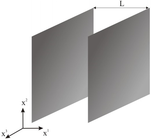
Figure 1: Two parallel planes with a separation of distance $L$ in the $x^{1}$ direction.

In this context, it is particularly useful to write the field $A_{\mu}$ on a plane wave basis using the Fourier sum over the directions parallel to the plates. Assuming that the directions $x^{2}$ y $x^{3}$ are compactified to large sizes $R_{2}$ y $R_{3}$ with periodic boundary conditions, we are able to obtain

$$A_{\mu}(x^{0},x^{1},x^{2},x^{3})=\sum_{\vec{k}}Ne^{i\vec{k}\cdot\vec{x}}A_{\mu}(x^{0},x^{1},k),$$ (2.2)

where it is valid that $A_{\mu}^{\dagger}(x^{0},x^{1},k)=A_{\mu}(x^{0},x^{1},-k)$ and $N$ is a constant that takes the value $\left[\sqrt{2\pi R_{2}R_{3}}\right]^{-1}$. Moreover, the vector $\vec{k}$ can be expressed for $n^{2},n^{3}=0,\pm 1,\pm 2,...,\pm\infty$ as

$$\vec{k}=\left(0,\frac{2\pi n^{2}}{R_{2}},\frac{2\pi n^{3}}{R_{3}}\right)\,.$$ (2.3)

The problem then decomposes into independent $(1+1)$-dimensional fields in the directions $x^{0},x^{1}$, labeled by $\vec{k}$. To study a fixed mode $\vec{k}$, without loss of generality, we can simplify the calculation by using a coordinate system adapted to $\vec{k}$, where $\hat{x}^{2}=\hat{k}$ and $\hat{x}^{3}=\hat{x}^{1}\crossproduct\hat{k}$. In these coordinates, the expression of the each mode is

$$Ne^{ikx_{2}}A_{\mu}(x_{0},x_{1},k)\,.$$ (2.4)

Considering the gauge freedom of the Maxwell field given by ${A^{\prime}}_{\mu}\rightarrow A_{\mu}+\partial_{\mu}\chi$ we also decompose $\chi$ in the plane wave basis. The mode corresponding to $\vec{k}$ writes

$$\chi(x_{0},x_{1},x_{2},x_{3})=Ne^{ikx_{2}}\chi(x_{0},x_{1},k)\,.$$ (2.5)

Then, a gauge transformation of a fix mode yields

$$A^{\prime}_{\mu}(x_{0},x_{1},x_{2},x_{3}) = Ne^{ikx_{2}}\left[(A_{0}(x_{0},x_{1},k)+\dot{\chi}(x_{0},x_{1},k))\hat{x}_{0}+\right.$$ (2.6)

$$+ \left.(A_{1}(x_{0},x_{1},k)+\partial_{1}\chi(x_{0},x_{1},k))\hat{x}_{1}\right.$$

$$+ \left.(A_{2}(x_{0},x_{1},k)+ik\chi(x_{0},x_{1},k))\hat{x}_{2}+A_{3}(x_{0},x_{1},k)\hat{x}_{3}\right]\,.$$

In the light of (2.6), it is clear that we can fix $\chi$ in such a way that the field component parallel to $\hat{k}$ vanishes, $A_{2}=0$. With this choice we have

$$F_{2\nu}=\partial_{2}A_{\nu}-\partial_{\nu}A_{2}=ikA_{\nu}\,.$$ (2.7)

In other words, in this gauge, and for each fixed mode $k$, $A_{\mu}$ can be expressed as a function of the gauge invariant tensor $F_{\mu\nu}$ in a way local in the coordinates $x^{0},x^{1}$. This allows us to identify the algebra of gauge invariant operators $F_{\mu\nu}$ in between the parallel planes with the one of the quantized gauge fixed operators $A_{\mu}$.

To proceed we compute the Hamiltonian. We must rewrite the Lagrangian (2.1) by using the expansion (2.4) under the proposed gauge condition. By doing so, we obtain for each mode the Lagrangian

$$\mathcal{L}_{k} = 1/2\left[\dot{A}^{\dagger}_{1}\dot{A}_{1}+\dot{A}^{\dagger}_{3}\dot{A}_{3}-k^{2}{A}^{\dagger}_{1}{A}_{1}-k^{2}{A}^{\dagger}_{3}{A}_{3}-\partial_{1}A_{3}^{\dagger}\partial_{1}A_{3}\right.$$ (2.8)

$$-\left.k^{2}{A}^{\dagger}_{0}{A}_{0}-\partial_{1}A_{0}^{\dagger}\partial_{1}A_{0}-A_{0}^{\dagger}\partial_{1}\dot{A}_{1}-\partial_{1}\dot{A}^{\dagger}_{1}A_{0}\right]\,.$$

The canonical momenta of the fields $A_{1}\,,A_{1}^{\dagger}\,,A_{3}\,,A_{3}^{\dagger}$ are given by

$$\pi_{1}=\frac{\partial\mathcal{L}_{k}}{\partial\dot{A}_{1}}=\frac{\dot{A}^{\dagger}_{1}}{2}+\frac{\partial_{1}A^{\dagger}_{0}}{2}\,\,,\,\,\pi_{3}=\frac{\partial\mathcal{L}_{k}}{\partial\dot{A}_{3}}=\frac{\dot{A}^{\dagger}_{3}}{2}\,,$$ (2.9)

$$\pi^{\dagger}_{1}=\frac{\partial\mathcal{L}_{k}}{\partial\dot{A}^{\dagger}_{1}}=\frac{\dot{A}_{1}}{2}+\frac{\partial_{1}A_{0}}{2}\,\,,\,\,\pi^{\dagger}_{3}=\frac{\partial\mathcal{L}_{k}}{\partial\dot{A}^{\dagger}_{3}}=\frac{\dot{A}_{3}}{2}\,.$$ (2.10)

The Hamiltonian of the mode is then given by the Legendre transform

$$\mathcal{H}_{k} = \pi_{1}\dot{A}_{1}+\pi^{\dagger}_{1}\dot{A}^{\dagger}_{1}+\pi_{3}\dot{A}_{3}+\pi^{\dagger}_{3}\dot{A}^{\dagger}_{3}-\mathcal{L}_{k}=2\pi_{1}^{\dagger}\pi_{1}+2\pi_{3}^{\dagger}\pi_{3}+\frac{k^{2}}{2}A^{\dagger}_{1}A_{1}+$$ (2.11)

$$+ \frac{k^{2}}{2}A^{\dagger}_{3}A_{3}+\frac{1}{2}\partial_{1}A^{\dagger}_{3}\partial_{1}A_{3}+\frac{k^{2}}{2}A^{\dagger}_{0}A_{0}+A^{\dagger}_{0}\partial_{1}\pi^{\dagger}_{1}+A_{0}\partial_{1}\pi_{1}$$

with the corresponding equal time commutation relations

$$\left[A_{1}(x_{0},x_{1},k),\pi_{1}({x}_{0},{x^{\prime}}_{1},k)\right]=i\delta(x_{1}-{x^{\prime}}_{1})\,,$$

$$\left[A_{3}(x_{0},x_{1},k),\pi_{3}({x}_{0},{x^{\prime}}_{1},k)\right]=i\delta(x_{1}-{x^{\prime}}_{1})\,.$$ (2.12)

It is clear from (2.11) that the field $A_{0}$ does not posses his own dynamic and thus it can be treated as a Lagrange multiplier. Differentiating, in order to obtain its equations of motion, we obtain the constraints

$$\partial_{1}\pi_{1}=-\frac{k^{2}}{2}A^{\dagger}_{0}\,\,,\,\,\partial_{1}\pi^{\dagger}_{1}=-\frac{k^{2}}{2}A_{0}\,.$$ (2.13)

Replacement of (2.13) in (2.11) gives

$$\mathcal{H}_{k}=2\pi_{1}^{\dagger}\pi_{1}+2\pi_{3}^{\dagger}\pi_{3}+\frac{k^{2}}{2}A^{\dagger}_{1}A_{1}+\frac{k^{2}}{2}A^{\dagger}_{3}A_{3}++\frac{1}{2}\partial_{1}A^{\dagger}_{3}\partial_{1}A_{3}+\frac{2}{k^{2}}\partial_{1}\pi_{1}\partial_{1}\pi^{\dagger}_{1}\,.$$ (2.14)

Making the identifications

$$\phi_{1}=\frac{\sqrt{2}\pi_{1}}{|k|}\,,\,P_{1}=-\frac{|k|A_{1}}{\sqrt{2}}\,,$$ (2.15)

$$\phi_{3}=\frac{A_{3}}{\sqrt{2}}\,,\,P_{3}=\sqrt{2}\pi_{3}\,,$$ (2.16)

where $\phi_{1},P_{1}$ and $\phi_{3},P_{3}$ are pairs of canonically conjugate variables, the Hamiltonian writes

$$\mathcal{H}_{k}=P^{\dagger}_{1}P_{1}+P^{\dagger}_{3}P_{3}+\partial_{1}\phi^{\dagger}_{1}\partial_{1}\phi_{1}+\partial_{1}\phi^{\dagger}_{3}\partial_{1}\phi_{3}+k^{2}\phi^{\dagger}_{1}\phi_{1}+k^{2}\phi^{\dagger}_{3}\phi_{3}\,.$$ (2.17)

This is exactly the Hamiltonian for the modes of two independent scalar fields $\phi_{1},\phi_{3}$ upon dimensional reduction (see for example [10]). As a result, the algebra of gauge invariant operators for the gauge field and the vacuum expectation values inside the parallel planes are identical to the algebras and expectation values corresponding to two massless scalar fields inside the same region.

To sum up, we conclude the EE of the Maxwell field associated with a region ${V}$ enclosed by two parallel planes is equivalent to the contribution of two independent scalar fields. In this way, we recover the known result obtained in [10] by working with the gauge invariant electric and magnetic fields directly. The entropy turns out to be [18]

$$S=c\frac{A}{\epsilon^{2}}-2\,k_{s}\frac{A}{L^{2}}\,,$$ (2.18)

where $A=R_{2}R_{3}$ is the area of the planes, $\epsilon$ is a short distance cutoff, $c$ a non universal constant, and $k_{s}$ is the universal coefficient corresponding to a scalar in this same geometry. This later can be computed with high precision from the knowledge of the one dimensional scalar entropy function [19]

$$k_{s}=0.0055351599...\,.$$ (2.19)

As we will now see, this exact identification of entropies between scalars and gauge fields does not hold for other regions.

3 Entanglement entropy for a Maxwell field in the sphere

We consider now the problem of a Maxwell field in the sphere, which also can be easily dimensionally reduced. Due to the spherical symmetry presented in this case we expand the field in question using scalar spherical harmonics for the $A_{0}$ component and vector spherical harmonics for $\vec{A}=(A_{1},A_{2},A_{3})$. That is

$$A_{0} = \sum_{lm}A^{0}_{lm}(t,r)Y_{lm}(\theta,\phi)\,,\quad l=0,1,...,\infty\,,\quad-l\leq m\leq l\,,$$ (3.1)

$$\vec{A} = \sum_{slm}A^{s}_{lm}(t,r)\overline{Y}_{lm}^{s}(\theta,\phi)\,,\quad l=0,1,...,\infty\,,\quad-l\leq m\leq l\,,\quad s=r,e,m\,,$$ (3.2)

where $\overline{Y}_{lm}^{s}$ are the vector spherical harmonics defined by

$$\overline{Y}_{lm}^{r}(\theta,\varphi) = Y_{lm}(\theta,\varphi)\hat{r}\,,\qquad l\geq 0,\quad-l\leq m\leq l\,,$$ (3.3)

$$\overline{Y}_{lm}^{e}(\theta,\varphi) = \frac{r\nabla Y_{lm}(\theta,\varphi)}{\sqrt{l(l+1)}}\,,\qquad l>0,\quad-l\leq m\leq l\,,$$ (3.4)

$$\overline{Y}_{lm}^{m}(\theta,\varphi) = \frac{\vec{r}\times\nabla Y_{lm}(\theta,\varphi)}{\sqrt{l(l+1)}}\,,\qquad l>0,\quad-l\leq m\leq l\,.$$ (3.5)

Considering the gauge transformations, it is useful to expand the function $\chi$ using scalar spherical harmonics as

$$\chi=\sum_{lm}\chi_{lm}(t,r)Y_{lm}(\theta,\phi)\,.$$ (3.6)

This gives the transformation law

$$\vec{A}^{\prime}=\sum_{lm}\left(A_{lm}^{r}+\partial_{r}\chi_{lm}\right)\overline{Y}_{lm}^{r}+\left(A_{lm}^{e}+\frac{\chi_{lm}}{r}\right)\overline{Y}_{lm}^{e}+A_{lm}^{m}\overline{Y}_{lm}^{m}\,.$$ (3.7)

We see it is possible to fix $\chi_{lm}$ completely in such way that the coefficient ${A^{\prime}}_{lm}^{e}$ of the “electric” vector spherical harmonics $\overline{Y}_{lm}^{e}$ is identically zero for each angular momentum. This particular choice of gauge is convenient because of other reasons too. It allow us to write for each mode

$$F_{e\mu}=\left(e^{\nu}\partial_{\nu}\right)A_{\mu}+\left(\partial_{\mu}e^{\nu}\right)A_{\nu}$$ (3.8)

where $e^{\mu}$ is the unit vector in the direction of $\overline{Y}_{lm}^{e}$, $e^{\mu}A_{\mu}$ represents the electric component of the vector $A_{\mu}$ that vanishes under this particular choice of gauge, and $e^{\mu}\partial_{\mu}$ is the derivative in such direction. The expression (3.8) shows that in this gauge we can recover $A_{\mu}$ on a sphere by the knowledge of the components $F_{e\mu}$ of the gauge invariant field tensor in the same sphere. This is because derivatives in (3.8) are tangential to the sphere. Therefore, even if the relation between the gauge fixed $A_{\mu}$ and $F_{\mu\nu}$ is non local in the angular directions, it maps the variables $A_{\mu}$ at fixed $r$ to physical variables with the same radius. This is a particular case of the general situation studied in [17] where it was shown that a gauge fixing that respects the localization of degrees of freedom in a region can be chosen such that $A_{\mu}$ vanishes on the boundary of the region in a direction parallel to the boundary itself. In the present example this direction is the one of the electric vector harmonics.

From this point, we proceed in the same way as in the case of parallel planes. In particular, a useful writing of the Lagrangian can be obtained by means of replacing (3.1) and (3.2) in (2.1), so as, by taking into consideration the orthonormality property of vector spherical harmonics, we get

$$L=\sum_{lm}\int_{0}^{\infty}dr\mathcal{L}_{lm}\,.$$ (3.9)

The Lagrangian $\mathcal{L}_{lm}$ for $l\geq 1$ follows from direct computation using the properties of vector harmonics listed in appendix A,

$$\mathcal{L}_{lm} = 1/2\left[r^{2}{\dot{A}_{l,m}^{r}}{\dot{A}_{l,-m}^{r}}+r^{2}{\dot{A}_{l,m}^{m}}{\dot{A}_{l,-m}^{m}}-l(l+1){{A}_{l,m}^{r}}{{A}_{l,-m}^{r}}\right.$$ (3.10)

$$-\left.l(l+1){{A}_{l,m}^{m}}{{A}_{l,-m}^{m}}-\left|{{A}_{l,m}^{m}}+r\partial_{r}{{A}_{l,m}^{m}}\right|^{2}+r^{2}\partial_{r}A^{0}_{l,m}\partial_{r}A^{0}_{l,-m}+l(l+1)A^{0}_{l,m}A^{0}_{l,-m}\right.$$

$$-\left.r^{2}A^{0}_{l,m}\partial_{r}{\dot{A}_{l,-m}^{r}}-r^{2}A^{0}_{l,-m}\partial_{r}{\dot{A}_{l,m}^{r}}+2rA^{0}_{l,m}{\dot{A}_{l,-m}^{r}}+2rA^{0}_{l,-m}{\dot{A}_{l,m}^{r}}\right]\,.$$

The Lagrangian density is independent of $m$, and to simplify the notation in the following we eliminate the index for $m$ in the variables and consider the real $m=0$ mode only, while we have to keep in mind that we will have $(2l+1)$ identical contributions to the EE for each angular momentum $l$.

The canonical conjugate momenta are defined by

$$\pi_{l}^{r}=\frac{\partial\mathcal{L}_{l}}{\partial{\dot{A}_{l}^{r}}}=r^{2}\left({\dot{A}_{l}^{r}}+\partial_{r}A^{0}_{l}\right)\,,\quad\pi_{l}^{m}=\frac{\partial\mathcal{L}_{l}}{\partial{\dot{A}_{l}^{m}}}=r^{2}{\dot{A}_{l}^{m}}\,.$$ (3.11)

which can be substituted in the Legendre transform

$$\mathcal{H}_{l}=\pi_{l}^{r}\dot{A}_{l}^{r}+\pi_{l}^{m}\dot{A}_{l}^{m}-\mathcal{L}_{l}\,,$$ (3.12)

in order to obtain the Hamiltonian

$$\mathcal{H}_{l}=\frac{\pi_{l}^{r}\pi_{l}^{r}}{2r^{2}}+\frac{\pi_{l}^{m}\pi_{l}^{m}}{2r^{2}}+l(l+1){{A}_{l}^{r}}{{A}_{l}^{r}}+l(l+1){{A}_{l}^{m}}{{A}_{l}^{m}}$$

$$+\left({{A}_{l}^{m}}+r\partial_{r}{{A}_{l}^{m}}\right)^{2}-\pi_{l}^{r}\partial_{r}A_{l}^{0}-\frac{l(l+1)}{2}A_{l}^{0}A_{l}^{0}\,.$$ (3.13)

The non trivial canonical commutation relations are given by

$$\left[{{A}_{l}^{r}}(t,r),{{\pi}_{l}^{r}}(t,r^{\prime})\right]=\left[{{A}_{l}^{m}}(t,r),{{\pi}_{l}^{m}}(t,r^{\prime})\right]=i\delta(r-r^{\prime})\,.$$ (3.14)

In addition, modes with different $l$ are independent to each other and their operators commute.

Again, $A_{l}^{0}$ is a Lagrange multiplier, allowing the derivation of the constraint

$$\partial_{r}\pi_{l}^{r}=l(l+1)A_{l}^{0}\,,$$ (3.15)

which can be replaced in (3.13) yielding

$$\mathcal{H}_{l} = \frac{1}{2}\left[\frac{\pi_{l}^{r}\pi_{l}^{r}}{r^{2}}+\frac{\partial_{r}\pi_{l}^{r}\partial_{r}\pi_{l}^{r}}{l(l+1)}+{l(l+1)}A_{l}^{r}A_{l}^{r}\right]$$ (3.16)

$$+ \frac{1}{2}\left[\frac{\pi_{l}^{m}\pi_{l}^{m}}{r^{2}}+2\left({{A}_{l}^{m}}+r\partial_{r}{{A}_{l}^{m}}\right)^{2}+{l(l+1)}A_{l}^{m}A_{l}^{m}\right]\,.$$

Lastly, the field and momentum variables can be rewritten as

$$\phi^{r}_{l} = \frac{\pi^{r}_{l}}{\sqrt{l(l+1)}}\,,\,\,\,P^{r}_{l}=-\sqrt{l(l+1)}A^{r}_{l}\,,$$ (3.17)

$$\phi^{m}_{l} = rA^{r}_{l}\,,\quad\qquad\,P^{m}_{l}=\frac{\pi_{l}^{m}}{r}\,,$$ (3.18)

and by applying (3.17) and (3.18) in (3.16) we reduce the Hamiltonian to the one of two identical radial modes given by

$$\mathcal{H}_{l} = \frac{1}{2}\left[P^{r}_{l}P^{r}_{l}+\partial_{r}\phi^{r}_{l}\partial_{r}\phi^{r}_{l}+\frac{l(l+1)}{r^{2}}\phi^{r}_{l}\phi^{r}_{l}\right]$$ (3.19)

$$+ \frac{1}{2}\left[P^{m}_{l}P^{m}_{l}+\partial_{r}\phi^{m}_{l}\partial_{r}\phi^{m}_{l}+\frac{l(l+1)}{r^{2}}\phi^{m}_{l}\phi^{m}_{l}\right]\,,$$

with the standard commutation relations

$$\left[{{\phi}_{l}^{r}}(t,r),{{P}_{l}^{r}}(t,r^{\prime})\right]=\left[{{\phi}_{l}^{m}}(t,r),{{P}_{l}^{m}}(t,r^{\prime})\right]=i\delta(r-r^{\prime})\,.$$ (3.20)

Each of these two identical modes has the same Hamiltonian as the one that results from the spherial reduction of a free massless scalar field [10, 20].

Eq. (3.10) does not apply to the zero angular momentum mode. This is simply because the electric (3.4) and magnetic (3.5) spherical harmonics do not exist for $l=0$. For $l=0$ we get the simpler expression

$$\mathcal{H}_{0}=\frac{\pi_{0}^{r}\pi_{0}^{r}}{2r^{2}}+A_{0}^{0}\partial_{r}\pi_{0}^{r}\,,$$ (3.21)

where by replacing the constraint $\partial_{r}\pi_{l=0}^{r}=0$, obtained from the equations of motion of $A^{0}_{0}$, we get

$$\mathcal{H}_{0}=\frac{\pi_{0}^{r}\pi_{0}^{r}}{2r^{2}}\,.$$ (3.22)

This means that the zero angular momentum mode does not have dynamics and thus generates no contributions to the entropy.

Therefore, the EE of the Maxwell field on the sphere is equivalent to the one of two scalar fields where the $l=0$ mode has been subtraced. This result coincides with the one given in [10]. The entanglement entropy of a scalar in a sphere has a universal logarithmic term $-1/90\log(R/\epsilon)$ [21, 22, 11, 23, 24]. The mode $l=0$ for the scalar (see the Hamiltonian (3.19) for $l=0$) corresponds to a massless $d=2$ field in the $r>0$ half-line with Dirichlet boundary condition at the origin, and its universal logarithmic entropy is $1/6\log(R/\epsilon)$ [10, 25]. The entropy of the Maxwell field in the sphere is then given by [10, 11]

$$S=c\frac{A}{\epsilon^{2}}-\frac{16}{45}\log(R/\epsilon)\,,$$ (3.23)

where the coefficient of the logarithmic term follows from $16/45=2\times 1/90+2\times 1/6$.

Here we recover this result by working with the gauge variant field $A_{\mu}$ instead of using directly the electric and magnetic gauge invariant fields as in [10]. It is important to remark that another gauge choice which does not respect the locality on the sphere would have given completely different incorrect results for the sphere EE.

4 Entanglement entropy of linearized gravitons between parallel planes

The free theory of a massless helicity $2$ particle can be described by a field $h_{\mu\nu}$. This field can be thought as describing metric perturbations $g_{\mu\nu}=\eta_{\mu\nu}+h_{\mu\nu}$ with respect to the Minkowski metric $\eta_{\mu\nu}$. The field $h_{\mu\nu}$ obeys the linearized Einstein equations and the Lagrangian that give these equations in absence of sources writes [26]

$$\mathcal{L}=-\partial_{\mu}h^{\mu\nu}\partial_{\alpha}h^{\alpha}_{\hphantom{\alpha}\nu}+\frac{1}{2}\partial^{\alpha}h_{\mu\nu}\partial_{\alpha}h^{\mu\nu}+\partial_{\mu}h^{\mu\nu}\partial_{\nu}h^{\alpha}_{\hphantom{\alpha}\alpha}-\frac{1}{2}\partial_{\alpha}h^{\mu}_{\hphantom{\mu}\mu}\partial^{\alpha}h^{\nu}_{\hphantom{\nu}\nu}\,.$$ (4.1)

The theory has a gauge invariance given by the transformation law

$$h^{\prime}_{\mu\nu}=h_{\mu\nu}+\partial_{\nu}\xi_{\mu}+\partial_{\mu}\xi_{\nu}\,,$$ (4.2)

for arbitrary vector field $\xi_{\mu}$. This corresponds to the diffeomorphism invariance of the Einstein theory of gravity at the linearized level.

The curvature is not gauge invariant in the non linear gravity theory but a gauge invariant operator corresponds to the linearized curvature tensor [27]

$$R_{\mu\nu\rho\sigma}=\frac{1}{2}\left[\partial_{\nu}\partial_{\rho}h_{\mu\sigma}-\partial_{\mu}\partial_{\rho}h_{\nu\sigma}+\partial_{\mu}\partial_{\theta}h_{\nu\rho}-\partial_{\nu}\partial_{\sigma}h_{\mu\rho}\right]\,.$$ (4.3)

It is a simple exercise to show that it is indeed invariant under (4.2). Therefore the theory of a helicity $2$ field in Minkowski space contains gauge invariant local operators, in contrast to what is expected in full quantum gravity. In consequence the EE is well defined, except for the usual issues about divergent terms. Let us study first the case of a region bounded by two parallel planes.

4.1 Plane wave decomposition and gauge fixing

For the wall between parallel planes we resort to a plane wave decomposition of the fields analogous to (2.4). Now we write for the field of a mode with $\vec{k}=k\hat{x}_{2}$

$$h_{\mu\nu}(x_{0},x_{1},x_{2},x_{3})=Ne^{ikx_{2}}h_{\mu\nu}(x_{0},x_{1},k)\,.$$ (4.4)

The arbitrary gauge function $\xi$ can also be decomposed in modes. The mode with vector $\vec{k}$ writes

$$\xi_{\mu}(x_{0},x_{1},x_{2},x_{3})=Ne^{ikx_{2}}\xi_{\mu}(x_{0},x_{1},k)\,.$$ (4.5)

Therefore, it can be easily observed that

$$h^{\prime}_{\mu\nu}=\begin{bmatrix}{h_{00}+2\dot{\xi_{0}}}&{h_{01}+\dot{\xi_{1}}+\partial_{1}\xi_{0}}&{h_{02}+\dot{\xi_{2}}+ik\xi_{0}}&{h_{03}+\dot{\xi_{3}}}\\ {h_{01}+\dot{\xi_{1}}+\partial_{1}\xi_{0}}&{h_{11}+2\partial_{1}\xi_{1}}&{h_{12}+\partial_{1}\xi_{2}+ik\xi_{2}}&{h_{13}+\partial_{1}\xi_{3}}\\ {h_{02}+\dot{\xi_{2}}+ik\xi_{0}}&{h_{12}+\partial_{1}\xi_{2}+ik\xi_{2}}&{h_{22}+2ik\xi_{2}}&{h_{23}+ik\xi_{3}}\\ {h_{03}+\dot{\xi_{3}}}&{h_{13}+\partial_{1}\xi_{3}}&{h_{23}+ik\xi_{3}}&{h_{33}}\end{bmatrix}\,,$$ (4.6)

making it clear that the components $h^{\prime}_{02}$, $h^{\prime}_{20}$, $h^{\prime}_{12}$, $h^{\prime}_{21}$, $h^{\prime}_{22}$, $h^{\prime}_{23}$, y $h^{\prime}_{32}$ can be fixed to zero if we use all the gauge freedom available. Now, all the components of $h^{\prime}_{\mu\nu}$ that have zero contractions in the direction of $\hat{k}$ are fixed to zero, allowing us to write the following component of the Riemann tensor for each mode as

$$2R_{2\mu 2\nu}=h_{\nu 2},_{\mu 2}+h_{2\mu},_{2\nu}-h_{\nu\mu},_{22}-h_{22},_{\mu\nu}=-h_{\nu\mu},_{22}=k^{2}h_{\nu\mu}\,.$$ (4.7)

That is, under this particular choice of gauge, it is possible to write the field $h_{\nu\mu}$ in terms of the Riemann tensor in a local way in the $x_{0}$ and $x_{1}$ coordinates. This means that the algebra of the gauge fixed degrees of freedom in $h_{\nu\mu}$ is the same as the algebra of the curvature tensor in between the planes.

4.2 Lagrangian for each momentum

The Lagrangian decomposes into independent modes for the different plane waves. Using the expansion (4.4) and the gauge condition presented in the previous section, the Lagrangian density for the $(1+1)$ dimensional theory of the mode $k$ can be expressed as

$$\mathcal{L}_{k} = \dot{h}_{13}\dot{h}_{13}^{\dagger}-\frac{1}{2}(\dot{h}_{11}\dot{h}_{33}^{\dagger}+\dot{h}_{33}\dot{h}_{11}^{\dagger})-k^{2}{h_{13}}{h_{13}}^{\dagger}+\frac{k^{2}}{2}({h_{11}}{h_{33}}^{\dagger}+{h_{33}}{h_{11}}^{\dagger})$$

$$-\frac{k^{2}}{2}h_{00}({h_{11}}^{\dagger}+{h_{33}}^{\dagger})-\frac{k^{2}}{2}({h_{11}}+{h_{33}})h_{00}^{\dagger}-h_{01}\partial_{1}\dot{h}_{33}^{\dagger}-\partial_{1}\dot{h}_{33}h_{01}^{\dagger}+h_{03}\partial_{1}\dot{h}_{13}^{\dagger}$$

$$+ \partial_{1}\dot{h}_{13}h_{03}^{\dagger}+k^{2}h_{03}h_{03}^{\dagger}+k^{2}h_{01}h_{01}^{\dagger}+\partial_{1}h_{03}\partial_{1}h_{03}^{\dagger}-\frac{1}{2}\partial_{1}h_{33}\partial_{1}h_{00}^{\dagger}-\frac{1}{2}\partial_{1}h_{00}\partial_{1}h_{33}^{\dagger}\,.$$

This Lagrangian contains two sets of independent fields and the problem can be split into two modes that will be treated separately. The first one contains the field $h_{13}$ and the Lagrange multiplier $h_{03}$

$$\mathcal{L}_{I}=\dot{h}_{13}\dot{h}_{13}^{\dagger}-k^{2}{h_{13}}{h_{13}}^{\dagger}-\partial_{1}h_{03}\dot{h}_{13}^{\dagger}-\dot{h}_{13}\partial_{1}h_{03}^{\dagger}+k^{2}h_{03}h_{03}^{\dagger}+\partial_{1}h_{03}\partial_{1}h_{03}^{\dagger}\,,$$ (4.9)

and the second one containing the fields $h_{11}$ y $h_{33}$ and the multipliers $h_{01}$ y $h_{00}$

$$\mathcal{L}_{II} = -\frac{1}{2}(\dot{h}_{11}\dot{h}_{33}^{\dagger}+\dot{h}_{33}\dot{h}_{11}^{\dagger})+\frac{k^{2}}{2}({h_{11}}{h_{33}}^{\dagger}+{h_{33}}{h_{11}}^{\dagger})+\partial_{1}h_{01}\dot{h}_{33}^{\dagger}+\dot{h}_{33}\partial_{1}h_{01}^{\dagger}$$

$$-\frac{k^{2}}{2}h_{00}({h_{11}}^{\dagger}+{h_{33}}^{\dagger})-\frac{k^{2}}{2}({h_{11}}+{h_{33}})h_{00}^{\dagger}+k^{2}h_{01}h_{01}^{\dagger}-\frac{1}{2}\partial_{1}h_{33}\partial_{1}h_{00}^{\dagger}-\frac{1}{2}\partial_{1}h_{00}\partial_{1}h_{33}^{\dagger}\,.$$

Therefore, the total Lagrangian is given by sum over modes

$$L=\sum_{k}\int_{0}^{\infty}dx_{1}\left(\mathcal{L}_{I}+\mathcal{L}_{II}\right)\,.$$ (4.11)

4.3 Hamiltonian of the mode I

The momenta $\pi_{13}$, $\pi_{13}^{\dagger}$ corresponding to the Lagrangian (4.9) are

$$\pi_{13}=\frac{\partial\mathcal{L}_{I}}{\partial\dot{h}_{13}}=\dot{h}_{13}^{\dagger}-\partial_{1}h_{03}^{\dagger}\quad,\quad\pi_{13}^{\dagger}=\frac{\partial\mathcal{L}_{I}}{\partial\dot{h}_{13}^{\dagger}}=\dot{h}_{13}-\partial_{1}h_{03}\,,$$ (4.12)

and the corresponding Hamiltonian is

$$\mathcal{H}_{I} = \pi_{13}\dot{h}_{13}+\pi_{13}^{\dagger}\dot{h}_{13}^{\dagger}-\mathcal{L}_{I}=$$ (4.13)

$$= \pi_{13}\pi_{13}^{\dagger}+k^{2}{h_{13}}{h_{13}}^{\dagger}-h_{03}\partial_{1}\pi_{13}-h_{03}^{\dagger}\partial_{1}\pi_{13}^{\dagger}-k^{2}h_{03}h_{03}^{\dagger}\,.$$

A constraint equation can be derived by computing the equation of motion of $h_{03}$

$$h_{03}=\frac{\partial_{1}\pi_{13}^{\dagger}}{k^{2}}\quad,\quad h_{03}^{\dagger}=\frac{\partial_{1}\pi_{13}}{k^{2}}\,,$$ (4.14)

which can be replaced in (4.13) to obtain

$$\mathcal{H}_{I}=\pi_{13}\pi_{13}^{\dagger}+k^{2}{h_{13}}{h_{13}}^{\dagger}+\frac{\partial_{1}\pi_{13}\partial_{1}\pi_{13}^{\dagger}}{k^{2}}\,.$$ (4.15)

In order to rewrite the Hamiltonian (4.15) as the one associated with a complex scalar (for each pair $\vec{k},-\vec{k}$) is convenient to define

$$\phi_{I}=\frac{\pi_{13}}{|k|}\quad,\quad P_{I}=-|k|h_{13}\,,$$ (4.16)

$$\phi_{I}^{\dagger}=\frac{\pi_{13}^{\dagger}}{|k|}\quad,\quad P_{I}^{\dagger}=-|k|h_{13}^{\dagger}\,.$$ (4.17)

In this way (4.15) gets

$$\mathcal{H}_{I}=P_{1}P_{1}^{\dagger}+k^{2}{\phi_{1}}{\phi_{1}}^{\dagger}+{\partial_{1}\phi_{1}\partial_{1}\phi_{1}^{\dagger}}\,.$$ (4.18)

Moreover, by canonical quantization of the field ${h_{13}}$ in (4.13), it is clear that the replacements (4.16) and (4.17) give $P_{1}$ and $\phi_{1}$ as canonically conjugate variables.

4.4 Hamiltonian of the mode II

Analyzing the dynamic of the fields $h_{00}$ y $h_{00}^{\dagger}$ in the Lagrangian (4.2) is evident that both play the role of Lagrange multipliers, giving rise to the constraints

$$\partial_{1}\partial_{1}h_{33}=k^{2}({h_{11}}+{h_{33}})\,,\quad\partial_{1}\partial_{1}h_{33}^{\dagger}=k^{2}({h_{11}}^{\dagger}+{h_{33}}^{\dagger})\,.$$ (4.19)

If we replace (4.19) in (4.2) it is possible to eliminate the field $h_{11}$ from the Lagrangian, obtaining

$$\mathcal{L}_{II} = \dot{h}_{33}\dot{h}_{33}^{\dagger}-k^{2}{h_{33}}{h_{33}}^{\dagger}+\frac{\partial_{1}\dot{h}_{33}\partial_{1}\dot{h}_{33}^{\dagger}}{k^{2}}$$ (4.20)

$$-\partial_{1}{h_{33}}\partial_{1}{h_{33}}^{\dagger}-h_{01}\partial_{1}\dot{h}_{33}^{\dagger}-\partial_{1}\dot{h}_{33}h_{01}^{\dagger}+k^{2}h_{01}h_{01}^{\dagger}\,.$$

The substitution produced a higher derivative term $k^{-2}\partial_{1}\dot{h_{33}}\partial_{1}\dot{h_{33}}^{\dagger}$. However, this problem disappear when we use the constraint equation related to the equation for the fields $h_{01}$ y $h_{01}^{\dagger}$ that also work as Lagrange multipliers. Indeed, we obtain

$$h_{01}=\frac{\partial_{1}\dot{h}_{33}}{k^{2}}\quad,\quad h_{01}^{\dagger}=\frac{\partial_{1}\dot{h}_{33}^{\dagger}}{k^{2}}\,.$$ (4.21)

Applying (4.21) in (4.20) the Lagrangian gets reduced to

$$\mathcal{L}_{II}=\dot{h}_{33}\dot{h}_{33}^{\dagger}-k^{2}{h_{33}}{h_{33}}^{\dagger}-\partial_{1}{h_{33}}\partial_{1}{h_{33}}^{\dagger}\,.$$ (4.22)

The canonical momenta associated to the complex field variables ${h_{33}}$ and ${h_{33}}^{\dagger}$ are

$$\pi_{33}=\frac{\partial\mathcal{L}_{II}}{\partial\dot{h}_{33}}=\dot{h}_{33}^{\dagger}\quad,\quad\pi_{33}^{\dagger}=\frac{\partial\mathcal{L}_{II}}{\partial\dot{h}_{33}^{\dagger}}=\dot{h}_{33}\,,$$ (4.23)

and the corresponding Hamiltonian gets the same form as (4.18),

$$\mathcal{H}_{II}=P_{II}P_{II}^{\dagger}+k^{2}{\phi_{II}}{\phi_{II}}^{\dagger}+{\partial_{1}\phi_{II}\partial_{1}\phi_{II}^{\dagger}}\,,$$ (4.24)

where we have introduced the trivial notation change

$$\phi_{II} = {h_{33}}\quad,\quad\,\,P_{II}=\pi_{13}\,,$$ (4.25)

$$\phi_{II}^{\dagger} = {h_{33}}^{\dagger}\quad,\quad P_{II}^{\dagger}=\pi_{13}^{\dagger}\,.$$ (4.26)

These variables also obey canonical commutation relations.

4.5 Entanglement Entropy

The Hamiltonians for the two modes (4.18) and (4.24) are equivalent to the ones of a dimensionally reduced scalar field, and to the two modes (2.17) for the Maxwell field. Therefore, we are allowed to conclude that the EE of linearized gravitons for the region enclosed between two parallel planes is equivalent to the one of two scalar fields or one Maxwell field. The universal coefficients will be the same in the three cases. We get again

$$S=c\frac{A}{\epsilon^{2}}-2\,k_{s}\frac{A}{L^{2}}\,,$$ (4.27)

with $k_{s}$ given by (2.19) [18].

5 Entanglement entropy of linearized gravitons in a sphere

In this section we treat the case of gravitons inside a sphere. We first introduce the tensor spherical harmonics which we use to decompose $h_{\mu\nu}$ in spherical coordinates. We also decompose the gauge transformations and choose a generic gauge adapted to the spherical symmetry that depends on three arbitrary constants. Then we expand the Lagrangian in terms of the gauge fixed field to get two independent radial modes for each $l,m$. The gauge choice is further refined to allow the simplification of the the mode Hamiltonians and to ensure locality in the radial direction in the relation between the gauge fixed field and the curvature tensor. We get a system of modes that are equivalent to the scalar spherical modes except that the $l=0,1$ modes are absent. Finally, we compute the entanglement entropy.

5.1 Tensor spherical harmonics

The tensor spherical harmonics are a further generalization of the concept of scalar and vector spherical harmonics that can be used as a basis for the space of symmetric tensors (of dimension six). An arbitrary symmetric tensor field $X$ can be expanded in polar coordinates as follows

$$X=\sum_{Jslm}X_{lm}^{Js}(r)T_{lm}^{Js}(\theta,\phi)\,,\,\,l=0,1,...,\infty\,,\,\,m=0,\pm 1,...,\pm l\,,\,\,Js=0l,0t,1e,1m,2e,2m\,,$$ (5.1)

where the tensor spherical harmonics $T_{lm}^{Js}$ are given by (see for example [28, 29])

$$T_{lm}^{0l} = \hat{r}\otimes\hat{r}Y_{lm}\,,\,\,\,\qquad\qquad\qquad\qquad T_{lm}^{0t}=\frac{1}{\sqrt{2}}\left(\delta-\hat{r}\otimes\hat{r}\right)Y_{lm}\,,$$

$$T_{lm}^{1e} = \sqrt{\frac{2}{l(l+1)}}r\left[\hat{r}\otimes\nabla Y_{lm}\right]^{S}\,,\,\,\quad\,\,\,T_{lm}^{1m}=\sqrt{\frac{2}{l(l+1)}}\left[\hat{r}\otimes\overline{r}\crossproduct\nabla Y_{lm}\right]^{S}\,,$$ (5.2)

$$T_{lm}^{2e} = \sqrt{2\frac{(l-2)!}{(l+2)!}}\left[r^{2}\nabla\nabla Y_{lm}\right]^{STT}\,,\,\,\,\,T_{lm}^{2m}=\sqrt{2\frac{(l-2)!}{(l+2)!}}\left[r\nabla\left(\overline{r}\crossproduct\nabla Y_{lm}\right)\right]^{STT}\,.$$

The spherical harmonics of spin $J=0$ are defined for $l\geq 0$, the ones related to spin $J=1$ for $l\geq 1$ and the in the case of spin $J=2$ for $l\geq 2$. In the notation of the equations (5.2) the symbol $\delta$ means the identity tensor $\delta_{ij}$. Additionally, the superscript $S$ means taking the symmetric part, and $TT$ the traceless part transverse to $\hat{r}$. For an arbitrary tensor $X_{ij}$ this later is given by the following expression

$$X_{ij}^{TT}=\left(\delta_{ik}-\hat{r}_{i}\hat{r}_{k}\right)\left(\delta_{jn}-\hat{r}_{j}\hat{r}_{n}\right)X_{kn}-\frac{1}{2}\left(\delta_{ij}-\hat{r}_{i}\hat{r}_{j}\right)\left[\left(\delta_{kn}-\hat{r}_{k}\hat{r}_{n}\right)X_{nk}\right]\,.$$ (5.3)

It will be useful to have a relation between tensor and vector spherical harmonics. This relation can be expressed as

$$T_{lm}^{0l} = \left[\hat{r}\otimes\overline{Y}_{lm}^{r}\right]^{S}\quad,\qquad\,\,T_{lm}^{0t}=\frac{1}{\sqrt{2}}\left(\delta Y_{lm}-\hat{r}\otimes\overline{Y}_{lm}^{r}\right)\,,$$

$$T_{lm}^{1e} = \sqrt{2}\left[\hat{r}\otimes\overline{Y}_{lm}^{e}\right]^{S}\quad,\quad T_{lm}^{1m}=\sqrt{2}\left[\hat{r}\otimes\overline{Y}_{lm}^{m}\right]^{S}\,,$$

$$T_{lm}^{2e} = \sqrt{\frac{2}{(l-1)(l+2)}}\left\{\left[r\nabla\overline{Y}_{lm}^{e}\right]^{S}+\frac{1}{\sqrt{2}}T_{lm}^{1e}+\sqrt{\frac{l(l+1)}{2}}T_{lm}^{0t}\right\}\,,$$ (5.4)

$$T_{lm}^{2m} = \sqrt{\frac{2}{(l-1)(l+2)}}\left\{\left[r\nabla\overline{Y}_{lm}^{m}\right]^{S}+\frac{1}{\sqrt{2}}T_{lm}^{1m}\right\}\,.$$

Further properties of the tensor spherical harmonics are listed in appendix B.

5.2 Decomposition of the spin 2 field in spherical harmonics

To make the process of computing the EE easier it will be useful to decompose the field $h_{\mu\nu}$ and the gauge arbitrary function $\xi_{\mu}$ in different basis with spherical symmetry. For this purpose we introduce the notation

$$h_{T}=\begin{bmatrix}{h_{11}}&{h_{12}}&{h_{13}}\\ {h_{21}}&{h_{22}}&{h_{23}}\\ {h_{31}}&{h_{32}}&{h_{33}}\end{bmatrix}\,\,,\,\,h_{V}=\begin{bmatrix}{h_{01}}\\ {h_{02}}\\ {h_{03}}\end{bmatrix}\,\,,\,\,h_{S}={h}_{00}\,\,,\,\,\xi_{V}=\begin{bmatrix}{\xi_{1}}\\ {\xi_{2}}\\ {\xi_{3}}\end{bmatrix}\,\,,\,\,\xi_{S}=\xi_{0}\,.$$ (5.5)

Firstly, we will work with the space-like part of the problem by expanding $h_{T}$ in tensor spherical harmonics and $\xi_{V}$ in vector spherical harmonics. Then we will study the time-like part by using vector spherical harmonics for $h_{V}$ and scalar spherical harmonics for $\xi_{S}$ and $h_{S}$.

5.3 Gauge fixing for the space-like components

As we just mention, $h_{T}$ y $\xi_{V}$ will be expanded using tensor and vector spherical harmonics respectively in the following way

$$h_{T}=\sum_{Jslm}h_{lm}^{Js}(t,r)T_{lm}^{Js}(\theta,\varphi)\quad,\quad\xi_{V}=\sum_{slm}\xi_{lm}^{s}(t,r)\overline{Y}_{lm}^{s}(\theta,\varphi)\,.$$ (5.6)

On the other hand, the gauge freedom of linear gravity can be expressed in this notation as

$$h^{\prime}_{T}=h_{T}+\nabla\xi_{V}+\left[\nabla\xi_{V}\right]^{T}=h_{T}+2\left[\nabla\xi_{V}\right]^{S}\,.$$ (5.7)

The combination of (5.6) and (5.7) gives

$$h^{\prime}_{T}=\sum_{Jslm}h_{lm}^{Js}T_{lm}^{Js}+2\sum_{slm}\left[\xi_{lm}^{s}\nabla\overline{Y}_{lm}^{s}+\overline{Y}_{lm}^{s}\otimes\partial_{r}\xi_{lm}^{s}\hat{r}\right]^{S}\,.$$ (5.8)

By computing $\xi_{lm}^{s}\nabla\overline{Y}_{lm}^{s}+\overline{Y}_{lm}^{s}\otimes\partial_{r}\xi_{lm}^{s}\hat{r}$ using the properties of vector and tensor spherical harmonics (appendices A and B), for $s=r,\,e,\,m$ separately, and then adding up these contributions we get

$$h^{\prime}_{T}=\sum_{lm}\left(h_{lm}^{0l}+2\partial_{r}\xi_{lm}^{r}\right)T^{0l}_{lm}+\left(h_{lm}^{0t}+\frac{2\sqrt{2}}{r}\xi_{lm}^{r}-\frac{\sqrt{2l(l+1)}}{r}\xi_{lm}^{e}\right)T_{lm}^{0t}$$

$$+\left(h_{lm}^{1e}+\frac{\sqrt{2l(l+1)}}{r}\xi_{lm}^{r}+\sqrt{2}\partial_{r}\xi_{lm}^{e}-\frac{\sqrt{2}}{r}\xi_{lm}^{e}\right)T^{1e}_{lm}+\left(h_{lm}^{1m}+\sqrt{2}\partial_{r}\xi_{lm}^{m}-\frac{\sqrt{2}}{r}\xi_{lm}^{m}\right)T^{1m}_{lm}$$

$$+\left(h_{lm}^{2e}+\frac{\sqrt{2(l-1)(l+2)}}{r}\xi_{lm}^{e}\right)T^{2e}_{lm}+\left(h_{lm}^{2m}+\frac{\sqrt{2(l-1)(l+2)}}{r}\xi_{lm}^{m}\right)T^{2m}_{lm}\,.$$ (5.9)

This particular case differs from the ones studied earlier because there are many possible reasonable choices of gauge fixing for the spherical waves, but, not all of them will allow us to calculate the EE that corresponds to the spherical boundary or allow us to decouple the two dynamical modes for each $lm$. More specifically, it can be seen that

• Fixing $\xi_{r}$ allows us to cancel the components that are parallel to $T_{lm}^{0t}$ or $T_{lm}^{1e}$ or to a linear combination of them.

• Fixing $\xi_{e}$ allows us to cancel the components that are parallel to $T_{lm}^{0t}$ or $T_{lm}^{2e}$ or to a linear combination of them.

• Fixing $\xi_{m}$ allows us to cancel the components that are parallel to $T_{lm}^{2m}$.

For now, we will use the freedom related to $\xi_{m}$ to cancel the ’electric-magnetic’ components, meaning that we take ${h^{\prime}}_{lm}^{2m}=0$ for all $l$ y $m$. Understanding the gauge fixing of $\xi_{r}$ y $\xi_{e}$ that is the correct one for our purposes is not simple at this stage. Because of that we choose to set to zero just some arbitrary linear combination of $T_{lm}^{0t}$, $T_{lm}^{1e}$ y $T_{lm}^{2e}$ to be further determined in what follows. There is only one resulting degree of freedom that we call $h_{l}^{te}$ that is associated with a linear combination of these tensors given by some undetermined coefficients. More formally, we fix the gauge such that

$$h_{T}=\sum_{lm}{h}^{0l}_{lm}T_{lm}^{0l}+{h}^{te}_{lm}\left(\alpha T_{lm}^{0t}+\beta T_{lm}^{1e}+\gamma T_{lm}^{2e}\right)+{h}^{1m}_{lm}T_{lm}^{1m}\,,$$ (5.10)

where $\alpha$, $\beta$ and $\gamma$ are constants.

5.4 Gauge fixing for the time-like components

In order to fix the gauge of the time-like part we will write the vector $h_{V}$ and the scalar $\xi_{S}$ as

$$h_{V}=\sum_{slm}h_{lm}^{0s}(t,r)\overline{Y}_{lm}^{s}(\theta,\varphi)\quad,\quad\xi_{S}=\sum_{lm}\xi^{0}_{lm}(t,r){Y}_{lm}(\theta,\varphi)\,.$$ (5.11)

For each component of $h_{V}$ we have ${h^{\prime}}_{0i}=h_{0i}+\partial_{0}\xi_{i}+\partial_{i}\xi_{0}$ or more conveniently ${h^{\prime}}_{V}=h_{V}+{\dot{\xi}}_{V}+\nabla\xi_{S}$. By replacing with (5.11) we get

$${h^{\prime}}_{V}=\sum_{lm}\left(h_{lm}^{0r}+\dot{\xi}^{r}_{lm}+\partial_{r}\xi^{0}_{lm}\right)\overline{Y}_{lm}^{r}+\left(h_{lm}^{0e}+\dot{\xi}^{e}_{lm}+\frac{\xi^{0}_{lm}}{r}\right)\overline{Y}_{lm}^{e}+\left(h_{lm}^{0m}+\dot{\xi}^{m}_{lm}\right)\overline{Y}_{lm}^{m}\,.$$ (5.12)

Thus, in analogy with the case of the Maxwell field can fix $\xi_{0}$ in such way that ${h^{\prime}}_{lm}^{0e}$ is zero for each $lm$, obtaining the expansion

$${h}_{T}=\sum_{lm}{h}_{lm}^{0r}\overline{Y}_{lm}^{r}+{h}_{lm}^{0m}\overline{Y}_{lm}^{m}\,.$$ (5.13)

5.5 Lagrangian for each angular momentum

The starting point is the Lagrangian (4.1). Using the decomposition of the field $h_{\mu\nu}$ given in (5.5) in terms of spatial and temporal components we obtain

$$\mathcal{L} = \left.\frac{1}{2}\left(\dot{h}_{T}\cdot\cdot\dot{h}_{T}-Tr\left({\dot{h}_{T}}\right)Tr\left({\dot{h}_{T}}\right)\right)+\frac{1}{2}\left(\nabla^{2}h_{T}\cdot\cdot h_{T}+\nabla Tr\left({h_{T}}\right)\cdot\nabla Tr\left({h_{T}}\right)\right)\right.$$

$$+\left.\left(\nabla\cdot h_{T}\right)\cdot\left[\left(\nabla\cdot h_{T}\right)-\nabla Tr\left({h_{T}}\right)\right]+\nabla h_{S}\left[(\nabla\cdot h_{T})-\nabla Tr\left({h_{T}}\right)\right]\right.$$

$$-\left.2\dot{h}_{V}\cdot\left[(\nabla\cdot h_{T})-\nabla Tr\left({h_{T}}\right)\right]-(\nabla\cdot h_{V})\cdot(\nabla\cdot h_{V})-\nabla^{2}h_{V}\cdot h_{V}\right.\,.$$

In this matricial notation a single dot means the contraction of a one index for each tensor and two dots the contraction of the two sets of indices of the two symmetric tensors involved in the product. The full Lagrangian is given by

$$L=\int_{\mathbb{R}}^{3}d^{3}\overline{x}\,\mathcal{L}=\int_{0}^{\infty}dr\,r^{2}\left(\int d\Omega\,\mathcal{L}\right)\,.$$ (5.15)

Replacing the expressions (5.10) and (5.13) in (5.5) and taking into account the properties of spherical harmonics (appendices A and B) it turns out we can rewrite the Lagrangian for independent modes for each $l$ y $m$

$$L=\sum_{lm}\int_{0}^{\infty}dr\,\left(\mathcal{L}^{I}_{lm}+\mathcal{L}^{II}_{lm}\right)\,,$$ (5.16)

where the $\mathcal{L}_{lm}^{I}$ contains the variables $h_{l}^{1m}$ and $h_{l}^{0m}$ and $\mathcal{L}_{lm}^{II}$ involves the fields $h_{l}^{0l}$ and $h_{l}^{te}$ together with the Lagrange multipliers $h_{l}^{0r}$ and $h_{l}^{00}$. The Lagrangians for the modes are independent of $m$, and it is clear that we will have $(2l+1)$ equal contributions for each $l$. Accordingly we will suppress the index $m$. After a long but straightforward calculation using the properties listed in appendices A and B, the Lagrangian corresponding to the mode $I$ (and $l\geq 2$) gets

$$\mathcal{L}_{l}^{I} = \frac{r^{2}}{2}\dot{h}^{1m}_{l}\dot{h}^{1m}_{l}-\frac{(l-1)(l+2)}{2}h_{l}^{1m}h_{l}^{1m}+r^{2}\partial_{r}h_{l}^{0m}\partial_{r}h_{l}^{0m}$$ (5.17)

$$+l(l+1)h_{l}^{0m}h_{l}^{0m}+\sqrt{2}\dot{h}^{1m}_{l}\left(rh_{l}^{0m}-r^{2}\partial_{r}h_{l}^{0m}\right)\,,$$

and the one associated with mode $II$ is

$$\mathcal{L}_{l}^{II} = \frac{r^{2}}{2}\left(\beta^{2}-\alpha^{2}+\gamma^{2}\right)\dot{h}^{te}_{l}\dot{h}^{te}_{l}-\sqrt{2}r^{2}\alpha\dot{h}^{0l}_{l}\dot{h}^{te}_{l}+\frac{r^{2}}{2}\left(\alpha^{2}-\gamma^{2}\right)\partial_{r}h_{l}^{te}\partial_{r}h_{l}^{te}$$ (5.18)

$$+ \sqrt{2}\alpha rh_{l}^{te}\partial_{r}h_{l}^{0l}+h_{l}^{0l}h_{l}^{0l}+\left(\beta^{2}-\frac{\sqrt{l(l+1)}}{2}\alpha\beta-\frac{\sqrt{(l-1)(l+2)}}{2}\beta\gamma\right)h_{l}^{te}h_{l}^{te}$$

$$+ \sqrt{2}\left(\frac{l(l+1)}{2}\alpha-\sqrt{l(l+1)}\beta+\frac{\sqrt{(l-1)l(l+1)(l+2)}}{2}\gamma\right)h_{l}^{0l}h_{l}^{te}+l(l+1)h_{l}^{0r}h_{l}^{0r}$$

$$+ h_{l}^{0r}\left[4r\dot{h}^{0l}_{l}-2\sqrt{2}\alpha r^{2}\partial_{r}\dot{h}^{te}_{l}-\sqrt{2}\left(2\alpha+\sqrt{l(l+1)}\beta\right)r\dot{h}^{te}_{l}\right]+h_{l}^{00}\left[-2r\partial_{r}h_{l}^{0l}\right.$$

$$- \left.(l(l+1)+2)h_{l}^{0l}+\sqrt{2}\alpha r^{2}\partial_{r}\partial_{r}h_{l}^{te}+\sqrt{2}\left(3\alpha+\sqrt{l(l+1)}\beta\right)r\partial_{r}h_{l}^{te}\right.$$

$$+ \left.\frac{1}{\sqrt{2}}\left(-(l-1)(l+2)\alpha+4\sqrt{l(l+1)}\beta-\sqrt{(l-1)l(l+1)(l+2)}\gamma\right)h_{l}^{te}\right]\,.$$

In the same way as for the case of parallel planes, we will study the modes $I$ and $II$ separately trying to reduce them to scalar fields for $l\geq 2$. Then we will present the particular cases $l=0$ and $l=1$.

5.6 Hamiltonian of mode I for $l\geq 2$

From equation (5.17) it can be seen clearly that $h_{l}^{0m}$ has no dynamic, thus we get the following constraint

$$-2r^{2}\partial_{r}\partial_{r}h_{l}^{0m}-4r\partial_{r}h_{l}^{0m}+2l(l+1)h_{l}^{0m}+\sqrt{2}r^{2}\dot{\partial_{r}h_{l}^{1m}}+3\sqrt{2}r\dot{h}^{1m}_{l}=0\,.$$ (5.19)

In an analogy with the parallel planes case in equation (5.19), this expression cannot be solved algebraically but the constraint can be implemented by first computing the Hamiltonian. The momenta are given by

$$\pi_{l}^{1m}=\frac{\partial\mathcal{L}^{I}_{l}}{\partial\dot{h}^{1m}_{l}}=r^{2}\dot{h}^{1m}_{l}+\sqrt{2}\left(rh_{l}^{0m}-r^{2}\partial_{r}h_{l}^{0m}\right)\,.$$ (5.20)

From equations (5.17) and (5.20) we compute

$$\mathcal{H}^{I}_{l} = \pi_{l}^{1m}\dot{h}^{1m}_{l}-\mathcal{L}^{I}_{lm}=\frac{\pi_{lm}^{1m}\pi_{lm}^{1m}}{2r^{2}}+\frac{(l-1)(l+2)}{2}h_{l}^{1m}h_{l}^{1m}$$ (5.21)

$$- (l-1)(l+2)h_{l}^{0m}h_{l}^{0m}-\sqrt{2}h_{l}^{0m}\left(\partial_{r}\pi_{lm}^{1m}+\frac{\pi_{lm}^{1m}}{r}\right)\,.$$

Now, by working with $h_{l}^{0m}$ as a Lagrange multiplier in (5.21) the following constraint appears

$$-2(l-1)(l+2)h_{l}^{0m}-\sqrt{2}\left(\partial_{r}\pi_{lm}^{1m}+\frac{\pi_{lm}^{1m}}{r}\right)=0\,.$$ (5.22)

Replacing (5.22) in (5.21) gives for $l\geq 2$

$$\mathcal{H}^{I}_{l}=\frac{l(l+1)}{2r^{2}}\frac{\pi_{l}^{1m}\pi_{l}^{1m}}{(l-1)(l+2)}+\frac{1}{2}\frac{\partial_{r}\pi_{l}^{1m}\partial_{r}\pi_{l}^{1m}}{(l-1)(l+2)}+\frac{1}{2}(l-1)(l+2)h_{l}^{1m}h_{l}^{1m}\,.$$ (5.23)

and by redefining the variables

$$\phi^{I}_{l}=\frac{\pi_{l}^{1m}}{\sqrt{(l-1)(l+2)}}\,,\qquad P^{I}_{l}=-\sqrt{(l-1)(l+2)}h_{l}^{1m}\,,$$ (5.24)

we reduce (5.23) to the Hamiltonian of a free scalar in the sphere

$$\mathcal{H}^{I}_{l}=\frac{1}{2}\left(P^{I}_{l}P^{I}_{l}+\partial_{r}\phi^{I}_{l}\partial_{r}\phi^{I}_{l}+\frac{l(l+1)}{r^{2}}\phi^{I}_{l}\phi^{I}_{l}\right)\,.$$ (5.25)

The canonical commutation relations

$$\left[P^{I}_{l}(t,r),\phi^{I}_{l}(t,r^{\prime})\right]=i\delta(r-r^{\prime})\,,$$ (5.26)

follow from

$$\left[\pi^{1m}_{l}(t,r),h^{1m}_{l}(t,r^{\prime})\right]=i\delta(r-r^{\prime})\,.$$ (5.27)

5.7 Hamiltonian of mode II for $l\geq 2$

For the mode II we have the Lagrangian (5.18), where working out the equations of motion of $h_{l}^{00}$ yields the constraint

$$-2r\partial_{r}h_{l}^{0l}-(l(l+1)+2)h_{l}^{0l}+\sqrt{2}\left(3\alpha+\sqrt{l(l+1)}\beta\right)r\partial_{r}h_{l}^{te}+\sqrt{2}\alpha r^{2}\partial_{r}\partial_{r}h_{l}^{te}$$

$$+\frac{1}{\sqrt{2}}\left(-(l-1)(l+2)\alpha+4\sqrt{l(l+1)}\beta-\sqrt{(l-1)l(l+1)(l+2)}\gamma\right)h_{l}^{te}=0\,.$$ (5.28)

Taking into account that (5.28) gives rise to non local terms (that can not be eliminated by the same means used for mode I), we are led to propose a particular gauge fixing such that

$$h_{l}^{0l}=ah_{l}^{te}+br\partial_{r}h_{l}^{te}\,,$$ (5.29)

with $a$ y $b$ constants that will be fixed to satisfy (5.28). Indeed, by replacing (5.29) in (5.28) we get

$$\sqrt{2}\left(\alpha-\sqrt{2}b\right)r^{2}\partial_{r}\partial_{r}h_{l}^{te}+\left(3\sqrt{2}\alpha+\sqrt{2l(l+1)}\beta-(l(l+1)+4)b-2a\right)r\partial_{r}h_{l}^{te}$$

$$\frac{1}{\sqrt{2}}\left(-(l-1)(l+2)\alpha+4\sqrt{l(l+1)}\beta-\sqrt{(l-1)l(l+1)(l+2)}\gamma\right.$$

$$\hskip 227.62204pt\left.-a\sqrt{2}(l(l+1)+2)\right)h_{l}^{te}=0\,.$$ (5.30)

It is possible to solve for $a$, $b$ and $\alpha$ in terms of $\beta$ and $\gamma$ in such a way that all the terms vanish separately. We get

$$a=\sqrt{\frac{2}{l(l+1)}}\beta-\sqrt{\frac{(l-1)(l+2)}{2l(l+1)}}\gamma\,,$$ (5.31)

$$b=\sqrt{\frac{2}{l(l+1)}}\beta+\sqrt{\frac{2}{(l-1)l(l+1)(l+2)}}\gamma\,,$$ (5.32)

$$\alpha=\frac{2}{\sqrt{l(l+1)}}\beta+\frac{2}{\sqrt{(l-1)l(l+1)(l+2)}}\gamma\,.$$ (5.33)

Eq. (5.33) then selects a particular gauge choice for achieving this simplification.

Replacing (5.29), (5.31), (5.32) y (5.33) in (5.18) and working with $h_{l}^{0r}$ as Lagrange multiplier allow us to obtain the following simple Lagrangian

$$\mathcal{L}^{II}_{l}=\frac{\gamma^{2}}{2}\left[\dot{h}^{te}_{l}\dot{h}^{te}_{l}-\partial_{r}h_{l}^{te}\partial_{r}h_{l}^{te}-l(l+1)h_{l}^{te}h_{l}^{te}\right]\,.$$ (5.34)

The corresponding Hamiltonian is

$$\mathcal{H}^{II}_{l}=\pi^{te}_{l}\dot{h}^{te}_{l}-\mathcal{L}^{II}_{l}=\frac{1}{2}\left[\frac{\pi^{te}_{l}\pi^{te}_{l}}{\gamma^{2}r^{2}}+\gamma^{2}r^{2}\partial_{r}h_{l}^{te}\partial_{r}h_{l}^{te}+\gamma^{2}l(l+1)h_{l}^{te}h_{l}^{te}\right]\,,$$ (5.35)

with the canonical commutation relations

$$\left[\pi^{te}_{l}(t,r),h^{te}_{l}(t,r^{\prime})\right]=i\delta(r-r^{\prime})\,.$$ (5.36)

Finally, by making the identifications

$$\phi^{II}_{l}=\gamma rh_{l}^{te}\quad,\quad P^{II}_{l}=\frac{\pi_{l}^{te}}{r\gamma}\,,$$ (5.37)

the Hamiltonian of the scalar field modes is recovered in the form

$$\mathcal{H}^{II}_{l}=\frac{1}{2}\left[P^{II}_{l}P^{II}_{l}+\partial_{r}\phi^{II}_{l}\partial_{r}\phi^{II}_{l}+\frac{l(l+1)}{r^{2}}\phi^{II}_{l}\phi^{II}_{l}\right]\,,$$ (5.38)

associated with the commutation relations

$$\left[P^{II}_{l}(t,r),\phi^{II}_{l}(t,r^{\prime})\right]=i\delta(r-r^{\prime})\,.$$ (5.39)

5.8 Analysis of the mode $l=0$

For the case $l=0$ the tensor spherical harmonics of spin $J=1$ y $J=2$ do not exist and the Lagrangian (5.15) reduces to

$$\mathcal{L}_{l=0}=\mathcal{L}_{l=0}^{I}+\mathcal{L}_{l=0}^{II}=-\frac{r^{2}}{2}\alpha^{2}\dot{h}^{te}_{0}\dot{h}^{te}_{0}-\sqrt{2}r^{2}\alpha\dot{h}^{0l}_{0}\dot{h}^{te}_{0}+\frac{r^{2}}{2}\alpha^{2}\partial_{r}h_{0}^{te}\partial_{r}h_{0}^{te}$$

$$+\sqrt{2}\alpha rh_{0}^{te}\partial_{r}h_{0}^{0l}+h_{0}^{0l}h_{0}^{0l}+2\sqrt{2}h_{0}^{0r}\left[\sqrt{2}r\dot{h}^{0l}_{0}-\alpha r^{2}\partial_{r}\dot{h}^{te}_{0}-\alpha r\dot{h}^{te}_{0}\right]$$ (5.40)

$$+\sqrt{2}h_{0}^{00}\left[-\sqrt{2}r\partial_{r}h_{l}^{0}{0l}-\sqrt{2}h_{0}^{0l}+\alpha r^{2}\partial_{r}\partial_{r}h_{0}^{te}+3\alpha r\partial_{r}h_{0}^{te}+\alpha h_{0}^{te}\right]\,.$$

The equation of motion of $h_{0}^{00}$ produces the constraint

$$-\sqrt{2}r\partial_{r}h_{0}^{0l}-\sqrt{2}h_{0}^{0l}+\alpha r^{2}\partial_{r}\partial_{r}h_{0}^{te}+3\alpha r\partial_{r}h_{0}^{te}+\alpha h_{0}^{te}=0\,.$$ (5.41)

By proposing the equivalent of (5.29) and replacing (5.41) we get that the constants $a$ y $b$ must be $a=b=\alpha/\sqrt{2}$ without the need of fixing $\alpha$, in other words

$$h_{0}^{0l}=\frac{\alpha}{\sqrt{2}}\left(h_{0}^{te}+r\partial_{r}h_{0}^{te}\right)\quad\forall\alpha\,.$$ (5.42)

On the other hand, taking $h_{0}^{0r}$ as Lagrange multiplier gives

$$\sqrt{2}r\dot{h}^{0l}_{0}-\alpha r^{2}\partial_{r}\dot{h}^{te}_{0}-\alpha r\dot{h}^{te}_{0}=0\,.$$ (5.43)

The equations (5.42) and (5.43) are clearly consistent with each other. Replacing both of them in (5.40) yields $\mathcal{L}_{l=0}=0$, allowing us to conclude that the $l=0$ mode makes no contribution to the EE for any choice of gauge.

5.9 Analysis of the mode $l=1$

For the case $l=1$ the tensor spherical harmonics of spin $J=0$ y $J=1$ are well defined but the ones corresponding to $J=2$ do not exist. Hence the Lagrangian for the mode $I$ now writes

$$\mathcal{L}_{l=1}^{I}=\frac{r^{2}}{2}\dot{h}^{1m}_{1}\dot{h}^{1m}_{1}+r^{2}\partial_{r}h_{1}^{0m}\partial_{r}h_{1}^{0m}+2h_{1}^{0m}h_{1}^{0m}+\sqrt{2}\dot{h}^{1m}_{1}\left(rh_{1}^{0m}-r^{2}\partial_{r}h_{1}^{0m}\right)\,.$$ (5.44)

In an analogous way to the case $l\geq 2$, we obtain $\pi_{1}^{1m}=r^{2}\dot{h}^{1m}_{1}+\sqrt{2}\left(rh_{1}^{0m}-r^{2}\partial_{r}h_{1}^{0m}\right)$ and the Hamiltonian can be expressed as

$$\mathcal{H}^{I}_{l=1}=\frac{\pi_{1}^{1m}\pi_{1}^{1m}}{2r^{2}}-\sqrt{2}h_{1}^{0m}\left(\partial_{r}\pi_{1}^{1m}+\frac{\pi_{1}^{1m}}{r}\right)\,.$$ (5.45)

Working with $h_{1}^{0m}$ as a multiplier gives

$$\mathcal{H}^{I}_{l=1}=\frac{\pi_{1}^{1m}\pi_{1}^{1m}}{2r^{2}}\,,\,\,\,\pi_{1}^{1m}=r\partial_{r}\pi_{1}^{1m}\,,$$ (5.46)

which implies that the mode $I$ will not contribute to the EE for $l=1$.

Moreover, the Lagrangian of mode $II$ can be given for $l=1$ from (5.18) as

$$\mathcal{L}_{l=1}^{II} = \frac{r^{2}}{2}\left(\beta^{2}-\alpha^{2}\right)\dot{h}^{te}_{1}\dot{h}^{te}_{1}-\sqrt{2}r^{2}\alpha\dot{h}^{0l}_{1}\dot{h}^{te}_{1}+\frac{r^{2}}{2}\alpha^{2}\partial_{r}h_{1}^{te}\partial_{r}h_{1}^{te}$$ (5.47)

$$+ \sqrt{2}\alpha rh_{1}^{te}\partial_{r}h_{1}^{0l}+h_{1}^{0l}h_{1}^{0l}+\left(\beta^{2}-\frac{\alpha\beta}{\sqrt{2}}\right)h_{1}^{te}h_{1}^{te}+\left(\sqrt{2}\alpha-2\beta\right)h_{1}^{0l}h_{1}^{te}$$

$$+ 2h_{1}^{0r}h_{1}^{0r}+2h_{1}^{0r}\left[2r\dot{h}^{0l}_{1}-\sqrt{2}\alpha r^{2}\partial_{r}\dot{h}^{te}_{1}-\left(\sqrt{2}\alpha+\beta\right)r\dot{h}^{te}_{1}\right]$$

$$+ h_{1}^{00}\left[-2r\partial_{r}h_{1}^{0l}-4h_{1}^{0l}+\sqrt{2}\alpha r^{2}\partial_{r}\partial_{r}h_{1}^{te}+\left(3\sqrt{2}\alpha+2\beta\right)r\partial_{r}h_{1}^{te}+4\beta h_{1}^{te}\right]\,.$$

so, $h_{1}^{00}$ yields the constraint

$$-2r\partial_{r}h_{1}^{0l}-4h_{1}^{0l}+\sqrt{2}\alpha r^{2}\partial_{r}\partial_{r}h_{1}^{te}+\left(3\sqrt{2}\alpha+2\beta\right)r\partial_{r}h_{1}^{te}+4\beta h_{1}^{te}=0\,.$$ (5.48)

In this calculation, we also propose the locality relation (5.29) and by replacing it in (5.48) we obtain that for every choice of gauge it is valid that

$$h_{1}^{0l}=\frac{\alpha}{\sqrt{2}}h_{1}^{te}+r\beta\partial_{r}h_{1}^{te}\quad\forall\,\alpha,\,\beta\,.$$ (5.49)

Finally, using (5.49) in (5.47) produces $\mathcal{L}_{l=1}^{II}=0$. Thus, there is no contribution of the mode $II$ for $l=1$.

5.10 Analysis of the gauge fixing

We have already restricted the gauge choice with the relation (5.33) that allow us to write the dynamics of the two modes in the same fashion as the one of the scalar modes. Now we analyze if the field $h_{\mu\nu}$ or, more conveniently, the resulting degrees of freedom associated with each mode $h_{l}^{1m}$ and $h_{l}^{te}$ can be written in terms of gauge invariant operators inside the sphere. For this purpose, we appeal to the expression (4.3) of the gauge invariant curvature tensor.

Using a computer based algebraic manipulation we obtain that the mode $I$ field given by $h_{l}^{1m}$ can be rewritten in terms of the "electric-radial-electric-magnetic" contraction of the Riemann tensor

$$R_{erem}^{lm}=e^{\mu}r^{\nu}e^{\rho}m^{\sigma}R_{\mu\nu\rho\sigma}^{lm}=F_{lm}(\theta,\varphi)\frac{h_{l}^{1m}(t,r)}{r^{2}}\,,$$ (5.50)

where $F_{lm}(\theta,\varphi)$ is a function of the angles $\theta$ and $\varphi$ for each $l$ and $m$. Specifically, for $m=0$ it is valid that

$$F_{l0}(\theta)=\frac{\pi^{\frac{5}{2}}l\sqrt{\Gamma^{3}(l+1)\Gamma(l)}}{16\Gamma^{2}(l+2)}P_{l}^{0}(\cos{\theta})[P_{l}^{1}(\cos{\theta})]^{3}\left(4P_{l}^{2}(\cos{\theta})\cot{\theta}+P_{l}^{3}(\cos{\theta})\right)\,,$$ (5.51)

where $P_{l}^{m}(\cos{\theta})$ are the associated Legendre polynomials. The important point in this expression is that the relation between $h_{l}^{1m}(t,r)$ and the curvature does not involve radial derivatives. That would make the algebra generated by this field non local with respect to the one of gauge invariant operators in the sphere.

For the mode $II$, under the partial gauge choice (5.33), we can further set $\alpha=0$ or equivalently

$$\gamma=-\frac{\beta}{\sqrt{(l-1)(l+2)}}\,,$$ (5.52)

to obtain locality with respect to the curvature tensor. With this choice (5.29) reduces to an algebraic relation (without any derivatives) between the fields $h_{l}^{0l}$ y $h_{l}^{te}$ given by

$$h_{l}^{0l}=\sqrt{\frac{(l-1)(l+2)}{2}}\beta h_{l}^{te}\,.$$ (5.53)

From this relation it follows that the remaining field $h_{l}^{te}$ can be computed from the "electric-magnetic-electric-magnetic" contraction of the Riemann tensor in a local way in $t,r$ as

$$R_{emem}^{lm}=e^{\mu}m^{\nu}e^{\rho}m^{\sigma}R_{\mu\nu\rho\sigma}^{lm}=G_{lm}(\theta,\varphi)\frac{h_{te}(t,r)}{r^{2}}\,,$$ (5.54)

where $G_{lm}(\theta,\varphi)$ is another function of the angles $\theta$, $\varphi$ for each $l$ and $m$. For $m=0$ it writes

$$G_{l0}(\theta) = \frac{\pi^{\frac{5}{2}}\beta\sqrt{l(l+2)\Gamma(l)}}{16(l+1)^{2}\sqrt{\Gamma(l+3)}}[P_{l}^{1}(\cos{\theta})]^{4}\left(4l(l+1)P_{l}^{0}(\cos{\theta})\right.$$ (5.55)

$$+\left.2(l(l+1)+2)P_{l}^{1}(\cos{\theta})\cot{\theta}+(l(l+1)+2)P_{l}^{2}(\cos{\theta})\right)\,.$$

Therefore, we conclude that, by taking $\alpha=0$, and eq. (5.52) for the gauge fixing, the gauge fixed field $h_{\mu\nu}$ inside the sphere generates the same algebra as the gauge invariant operators. This algebra is equivalent to the one of the modes of two scalar fields except for the $l=0,1$ modes which are absent for the helicity $2$ theory.

5.11 Entanglement entropy and logarithmic coefficient

To sum up, the EE associated with linearized gravitons in a sphere of radius $R$ is equivalent to the one corresponding to two scalar fields without contributions of the $l=0$ and $l=1$ angular momentum modes (or a Maxwell field without the $l=1$ modes).

As we recall in section 3, the entanglement entropy of a scalar in a sphere has a universal logarithmic term $-1/90\log(R/\epsilon)$ and the mode $l=0$ for the scalar corresponds to a massless $d=2$ scalar field in the $r>0$ half-line with entropy given by $1/6\log(R/\epsilon)$. To obtain the universal logarithmic term for gravitons we just need the logarithmic contribution of the $l=1$ mode for the scalar.

This mode is a $d=2$ field in the half-line $r>0$ with Hamiltonian

$$\mathcal{H}=\frac{1}{2}\left[P^{2}+(\partial_{r}\phi)^{2}+\frac{2}{r^{2}}\phi^{2}\right]\,.$$ (5.56)

This model is scale invariant, but in contrast with the $d=2$ scalar field it contains a potential term $2/r^{2}\phi^{2}$. We have to compute the entanglement entropy in an interval $r\in(0,R)$. The ultraviolet divergent piece of the EE comes from entanglement in high energy fluctuations around the boundary $r=R$. For these high energy fluctuations the effect of the potential can be neglected and then we must have a divergent piece that is the same as for the usual scalar field $S\sim-1/6\,\log(\epsilon)$. As the model does not contain any dimensionfull scales by dimensional reasons we obtain

$$S=\frac{1}{6}\,\log(R/\epsilon)+\textrm{cons}\,.$$ (5.57)

We have check this numerically in the lattice to an excellent (five digits) precision.

Hence, as for the $l=0$ mode, we get a $1/6$ coefficient for the logarithmic term of the $l=1$ modes. Consequently, summing up, we get a logarithmic coefficient for the graviton in the sphere given by twice the coefficient of the scalar subtracting two times the $l=0$ mode and $2(2l+1)=6$ times the $l=1$ mode, obtaining

$$2\times\left(-\frac{1}{90}-\frac{1}{6}-3\times\frac{1}{6}\right)=-\frac{61}{45}\,.$$ (5.58)

As it seems to be the rule, the value of the logarithmic coefficient increases with spin, being higher for helicity $2$ than for Maxwell and scalar fields. The entropy on the sphere then writes

$$S=c\frac{A}{\epsilon^{2}}-\frac{61}{45}\,\log(R/\epsilon)\,.$$ (5.59)

6 Discussion

We have computed the EE for free gravitons in flat space for a region between parallel planes and for the sphere. For the wall we find a universal coefficient that coincides with the one of two scalar fields. For the sphere the logarithmic term is given by $-61/45$, that is equivalent to two scalar fields where the $l=0$ and $l=1$ modes are missing. These results refer to clear physical quantities. First, our real time approach allow us to clarify that these are entropies of gauge invariant operator algebras of the theory inside the regions. Second, the meaning of these universal terms for the continuum model follows from the fact that they coincide with the ones obtained using the mutual information. We can write a regularized entropy as [31],

$$S_{\epsilon}(A)\equiv\frac{1}{2}\,I_{\epsilon}(A_{+},A_{-})\,.$$ (6.1)

In this formula one computes the mutual information between two regions $A_{+}$ and $A_{-}$ covering most of the inside and outside parts of the boundary of $A$ respectively, but symmetrically separated from the boundary by a distance $\epsilon/2$. This can be thought a form of point splitting regularization of the entropy. The mutual information for disjoint regions is completely unambiguos in QFT and thus is $S_{\epsilon}(A)$. In particular, mutual information is unaffected by details of the algebra definition such as center terms (or edge modes). In the present case our results for the entropy are indeed equivalent to $S_{\epsilon}(A)$. This is the case of the full scalar field EE [10] and this identification also holds for the $l=0,1$ modes. These later one dimensional fields have mutual information that diverge as $-1/3\log(\epsilon)$ as the boundaries of $A_{+}$ and $A_{-}$ approach each other. This holds for the free scalar and this UV result cannot change due to the potential or the boundary condition at the origin.

There are other results in the literature concerning the logarithmic coefficient due to gravitons, specially in black hole backgrounds (see for example [33, 8, 9, 34]; see also [36] and references therein for gravitons in de Sitter space). There is the general expectation that the logarithmic coefficient for the sphere should be proportional to the $A$ anomaly [21, 23]. The free graviton does not have a symmetric gauge invariant stress tensor due to the Weinberg Witten theorem [35], and then the definition of the $A$ anomaly is uncertain. For a Maxwell field there is a mismatch of the logarithmic term in the entanglement entropy and the $A$ anomaly which is solved by coupling the theory to (heavy) charges. In the present case a clarification of what is the right coefficient for interacting gravity seems to be further away since any interactions would take us away from the QFT setting, and thus rising the problems of operator algebra localization. Eternal black holes seem to be a more natural setup in gravity than the sphere since they are related to a partition of the asymptotic space in two. In this same sense, there are also indications that in full quantum gravity a boundary separating localized degrees of freedom should be an extremal surfaces [1, 37]. This is of course the case of the entanglement wedge in holographic EE but not the sphere is Minkowski space.

A natural conjecture that suggest itself from our results for the Maxwell field and the graviton is that on the sphere the EE of higher helicity $h>2$ fields should be equivalent to the one of two scalar fields where the $l=0,\cdots,h-1$ modes are subtracted. By the same reasons discussed in the previous section these modes have a EE given by

$$S=\frac{1}{6}\,\log(R/\epsilon)+\textrm{f(l)}\,,$$ (6.2)

where $f(l)$ is a function of the angular momentum. Hence, we would have a logarithmic coefficient

$$-2\left(\frac{1}{90}+\frac{1}{6}\sum_{l=0}^{h-1}(2l+1)\right)=-\frac{1+15h^{2}}{45}\,.$$ (6.3)

Another interesting problem is how to fix the gauge for the graviton in order that $h^{\mu\nu}$ inside a region of arbitrary shape is given in terms of the gauge invariant operators localized in the same region. We hope to come back to these problems in the future.

Appendix A Properties of vector spherical harmonics

In this appendix we list some useful properties of vector spherical harmonics, some of then may also be found in [10, 28, 29]. The vector spherical harmonics are defined by (3.3,3.4,3.5). They satisfy the orthogonality relations

$$\int\overline{Y}_{lm}^{s}\overline{Y}_{lm}^{s^{\prime}*}d\Omega=\delta_{ss^{\prime}}\delta_{ll^{\prime}}\delta_{mm^{\prime}}\,,$$ (A.1)

where $\overline{Y}_{lm}^{s*}$ is the complex conjugate of $\overline{Y}_{lm}^{s}$, that is also given by

$$\overline{Y}_{lm}^{s*}=(-1)^{m}\overline{Y}_{l(-m)}^{s}\,.$$ (A.2)

The vector spherical harmonics can be used to expand and arbitrary three component vector $\overline{V}$ as

$$\overline{V}=\sum_{l=0}^{\infty}\sum_{m=-l}^{l}\sum_{s=r,e,m}V^{s}_{lm}(r)\overline{Y}_{lm}^{s}(\theta,\varphi)$$ (A.3)

where the functions $V^{s}_{lm}(r)$ are fixed by the Fourier coefficient expression

$$V^{s}_{lm}(r)=\int\overline{V}\cdot\overline{Y}^{s^{*}}_{lm}d\Omega\,.$$ (A.4)

The vector spherical harmonics posses the following directional properties

$$\hat{r}\cdot\overline{Y}_{lm}^{r}=Y_{lm},\quad\hat{r}\cdot\overline{Y}_{lm}^{e}=0,\quad\hat{r}\cdot\overline{Y}_{lm}^{m}=0\,.$$ (A.5)

and their divergences are given by

$$\nabla\cdot\overline{Y}_{lm}^{r} = \frac{2}{r}Y_{lm}\,,$$ (A.6)

$$\nabla\cdot\overline{Y}_{lm}^{e} = -\frac{\sqrt{l(l+1)}}{r}Y_{lm}\,,$$ (A.7)

$$\nabla\cdot\overline{Y}_{lm}^{m} = 0\,.$$ (A.8)

The curls can be written as

$$\nabla\crossproduct\overline{Y}^{r}_{lm} = -\frac{\sqrt{l(l+1)}}{r}\overline{Y}^{m}_{lm}\,,$$ (A.9)

$$\nabla\crossproduct\overline{Y}^{e}_{lm} = \frac{1}{r}\overline{Y}^{m}_{lm}\,,$$ (A.10)

$$\nabla\crossproduct\overline{Y}^{m}_{lm} = -\frac{\sqrt{l(l+1)}}{r}\overline{Y}^{r}_{lm}-\frac{1}{r}\overline{Y}^{e}_{lm}\,.$$ (A.11)

Finally, the Laplancians can be computed to be

$$\nabla^{2}\overline{Y}_{lm}^{r} = -\frac{l(l+1)+2}{r^{2}}\overline{Y}_{lm}^{r}+\frac{2\sqrt{l(l+1)}}{r^{2}}\overline{Y}_{lm}^{e}\,,$$ (A.12)

$$\nabla^{2}\overline{Y}_{lm}^{e} = \frac{2\sqrt{l(l+1)}}{r^{2}}\overline{Y}_{lm}^{r}-\frac{l(l+1)}{r^{2}}\overline{Y}_{lm}^{e}\,,$$ (A.13)

$$\nabla^{2}\overline{Y}_{lm}^{m} = -\frac{l(l+1)}{r^{2}}\overline{Y}_{lm}^{m}\,.$$ (A.14)

Appendix B Properties of tensor spherical harmonics

In this appendix we list some properties of tensor spherical harmonics, some of then may also be found in [28, 29]. They are given by eqs. (5.2) or alternatively by the expressions (5.4). Their most useful characteristic is that they can be used as a basis for the space of symmetric tensors fields at a fixed radius. The tensor spherical harmonics satisfy the orthogonality relation

$$\int Tr\left({T_{lm}^{JS}{T^{*}}_{l^{\prime}m^{\prime}}^{J^{\prime}S"}}\right)d\Omega=\delta_{JJ^{\prime}}\delta_{ss^{\prime}}\delta_{ll^{\prime}}\delta_{mm^{\prime}}\,,$$ (B.1)

where ${T^{*}}_{lm}^{JS}$ is the complex conjugate of ${T}_{lm}^{JS}$ given by

$${T^{*}}_{lm}^{JS}=(-1)^{m}T_{l-m}^{JS}\,.$$ (B.2)

The traces of the tensor spherical harmonics are

$$Tr\left({T_{lm}^{0l}}\right)=Y_{lm}\,,\qquad Tr\left({T_{lm}^{0t}}\right)=\sqrt{2}Y_{lm}\,,$$

$$Tr\left({T_{lm}^{Js}}\right)=0\,,\qquad Js=1e,1m,2e,2m\,.$$ (B.3)

They further satisfy

$$\hat{r}\cdot T_{lm}^{0l}=\overline{Y}_{lm}^{r}\,,\qquad\hat{r}\cdot T_{lm}^{1e}=\frac{1}{\sqrt{2}}\overline{Y}_{lm}^{e}\,,\qquad\hat{r}\cdot T_{lm}^{2e}=0\,,$$

$$\hat{r}\cdot T_{lm}^{0t}=0\,,\qquad\hat{r}\cdot T_{lm}^{1m}=\frac{1}{\sqrt{2}}\overline{Y}_{lm}^{m}\,,\qquad\hat{r}\cdot T_{lm}^{2m}=0\,.$$ (B.4)

The divergences of tensor spherical harmonics can be written as

$$\nabla\cdot T_{lm}^{0l} = \frac{2}{r}\overline{Y}_{lm}^{r}\,,$$ (B.5)

$$\nabla\cdot T_{lm}^{0t} = -\frac{\sqrt{2}}{r}\overline{Y}_{lm}^{r}+\frac{1}{r}\sqrt{\frac{l(l+1)}{2}}\overline{Y}_{lm}^{e}\,,$$ (B.6)

$$\nabla\cdot T_{lm}^{1e} = -\frac{1}{r}\sqrt{\frac{l(l+1)}{2}}\overline{Y}_{lm}^{r}+\frac{1}{r}\frac{3}{\sqrt{2}}\overline{Y}_{lm}^{e}\,,$$ (B.7)

$$\nabla\cdot T_{lm}^{1m} = \frac{1}{r}\frac{3}{\sqrt{2}}\overline{Y}_{lm}^{m}\,,$$ (B.8)

$$\nabla\cdot T_{lm}^{2e} = -\frac{1}{r}\sqrt{\frac{(l-1)(l+2)}{2}}\overline{Y}_{lm}^{e}\,,$$ (B.9)

$$\nabla\cdot T_{lm}^{2m} = -\frac{1}{r}\sqrt{\frac{(l-1)(l+2)}{2}}\overline{Y}_{lm}^{m}\,,$$ (B.10)

and the Laplacians are the following

$$\nabla^{2}T_{lm}^{0l} = -\frac{l(l+1)+4}{r^{2}}T_{lm}^{0l}+\frac{2\sqrt{2}}{r^{2}}T_{lm}^{0t}+\frac{2\sqrt{2l(l+1)}}{r^{2}}T_{lm}^{1e}\,,$$ (B.11)

$$\nabla^{2}T_{lm}^{0t} = \frac{2\sqrt{2}}{r^{2}}T_{lm}^{0l}-\frac{l(l+1)+2}{r^{2}}T_{lm}^{0t}-\frac{2\sqrt{l(l+1)}}{r^{2}}T_{lm}^{1e}\,,$$ (B.12)

$$\nabla^{2}T_{lm}^{1e} = \frac{2\sqrt{2l(l+1)}}{r^{2}}T_{lm}^{0l}-\frac{2\sqrt{l(l+1)}}{r^{2}}T_{lm}^{0t}$$ (B.13)

$$-\frac{l(l+1)+4}{r^{2}}T_{lm}^{1e}+\frac{2\sqrt{(l-1)(l+2)}}{r^{2}}T_{lm}^{2e}\,,$$

$$\nabla^{2}T_{lm}^{1m} = -\frac{l(l+1)+4}{r^{2}}T_{lm}^{1m}+\frac{2\sqrt{(l-1)(l+2)}}{r^{2}}T_{lm}^{2m}\,,$$ (B.14)

$$\nabla^{2}T_{lm}^{2e} = \frac{2\sqrt{(l-1)(l+2)}}{r^{2}}T_{lm}^{1e}-\frac{(l-1)(l+2)}{r^{2}}T_{lm}^{2e}\,,$$ (B.15)

$$\nabla^{2}T_{lm}^{2m} = \frac{2\sqrt{(l-1)(l+2)}}{r^{2}}T_{lm}^{1m}-\frac{(l-1)(l+2)}{r^{2}}T_{lm}^{2m}\,.$$ (B.16)

References

• [1] J. Camps, “Superselection Sectors of Gravitational Subregions,” JHEP 1901, 182 (2019) [arXiv:1810.01802 [hep-th]].
• [2] W. Donnelly and S. B. Giddings, Phys. Rev. D 96, 086013 (2017) [arXiv:1706.03104 [hep-th]].
• [3] S. Ryu and T. Takayanagi, “Holographic derivation of entanglement entropy from AdS/CFT,” Phys. Rev. Lett.  96, 181602 (2006) [hep-th/0603001].
• [4] T. Faulkner, A. Lewkowycz and J. Maldacena, “Quantum corrections to holographic entanglement entropy,” JHEP 1311, 074 (2013) [arXiv:1307.2892 [hep-th]].
• [5] B. Czech, J. L. Karczmarek, F. Nogueira and M. Van Raamsdonk, “The Gravity Dual of a Density Matrix,” Class. Quant. Grav.  29, 155009 (2012) [arXiv:1204.1330 [hep-th]].
• [6] D. L. Jafferis, A. Lewkowycz, J. Maldacena and S. J. Suh, “Relative entropy equals bulk relative entropy,” JHEP 1606, 004 (2016) [arXiv:1512.06431 [hep-th]].
• [7] X. Dong, D. Harlow and A. C. Wall, “Reconstruction of Bulk Operators within the Entanglement Wedge in Gauge-Gravity Duality,” Phys. Rev. Lett.  117, no. 2, 021601 (2016) [arXiv:1601.05416 [hep-th]].
• [8] S. N. Solodukhin, “Entanglement entropy of black holes,” Living Rev. Rel.  14, 8 (2011) [arXiv:1104.3712 [hep-th]].
• [9] A. Sen, “Logarithmic Corrections to Schwarzschild and Other Non-extremal Black Hole Entropy in Different Dimensions,” JHEP 1304, 156 (2013) [arXiv:1205.0971 [hep-th]].
• [10] H. Casini and M. Huerta, “Entanglement entropy of a Maxwell field on the sphere,” Phys. Rev. D 93, no. 10, 105031 (2016) [arXiv:1512.06182 [hep-th]].
• [11] J. S. Dowker, “Entanglement entropy for even spheres,” arXiv:1009.3854 [hep-th].
• [12] K. W. Huang, “Central Charge and Entangled Gauge Fields,” Phys. Rev. D 92, no. 2, 025010 (2015) doi:10.1103/PhysRevD.92.025010 [arXiv:1412.2730 [hep-th]].
• [13] H. Casini, M. Huerta, J. M. Magán and D. Pontello, “Entanglement entropy and superselection sectors I. Global symmetries,” arXiv:1905.10487 [hep-th].
• [14] H. Casini, M. Huerta, J. M. Magán and D. Pontello, “On the logarithmic coefficient of the entanglement entropy of a Maxwell field,” to appear.
• [15] W. Donnelly and A. C. Wall, “Geometric entropy and edge modes of the electromagnetic field,” Phys. Rev. D 94, no. 10, 104053 (2016) [arXiv:1506.05792 [hep-th]].
• [16] S. Ghosh, R. M. Soni and S. P. Trivedi, “On The Entanglement Entropy For Gauge Theories,” JHEP 1509, 069 (2015) [arXiv:1501.02593 [hep-th]].
• [17] H. Casini, M. Huerta and J. A. Rosabal, “Remarks on entanglement entropy for gauge fields,” Phys. Rev. D 89, no. 8, 085012 (2014) [arXiv:1312.1183 [hep-th]].
• [18] H. Casini and M. Huerta, “Entanglement and alpha entropies for a massive scalar field in two dimensions,” J. Stat. Mech.  0512, P12012 (2005) [cond-mat/0511014].
• [19] H. Casini and M. Huerta, “Entanglement entropy in free quantum field theory,” J. Phys. A 42, 504007 (2009) [arXiv:0905.2562 [hep-th]].
• [20] M. Srednicki, “Entropy and area,” Phys. Rev. Lett.  71, 666 (1993) [hep-th/9303048].
• [21] S. N. Solodukhin, “Entanglement entropy, conformal invariance and extrinsic geometry,” Phys. Lett. B 665, 305 (2008) [arXiv:0802.3117 [hep-th]].
• [22] H. Casini and M. Huerta, “Entanglement entropy for the n-sphere,” Phys. Lett. B 694, 167 (2011) [arXiv:1007.1813 [hep-th]].
• [23] H. Casini, M. Huerta and R. C. Myers, “Towards a derivation of holographic entanglement entropy,” JHEP 1105, 036 (2011) [arXiv:1102.0440 [hep-th]].
• [24] R. Lohmayer, H. Neuberger, A. Schwimmer and S. Theisen, “Numerical determination of entanglement entropy for a sphere,” Phys. Lett. B 685, 222 (2010) [arXiv:0911.4283 [hep-lat]].
• [25] P. Calabrese and J. L. Cardy, “Entanglement entropy and quantum field theory,” J. Stat. Mech.  0406, P06002 (2004) [hep-th/0405152].
• [26] T. Ortin, “Gravity and strings,” doi:10.1017/CBO9780511616563
• [27] C. W. Misner, K. S. Thorne and J. A. Wheeler, “Gravitation,” W. H. Freeman and Company, San Francisco 1973, 1279p
• [28] G. Compère, R. Oliveri and A. Seraj, “Gravitational multipole moments from Noether charges,” JHEP 1805, 054 (2018) [arXiv:1711.08806 [hep-th]].
• [29] K. S. Thorne, “Multipole Expansions of Gravitational Radiation,” Rev. Mod. Phys.  52, 299 (1980).
• [30] T. Regge and J. A. Wheeler, “Stability of a Schwarzschild singularity,” Phys. Rev.  108, 1063 (1957).
• [31] H. Casini, M. Huerta, R. C. Myers and A. Yale, “Mutual information and the F-theorem,” JHEP 1510, 003 (2015) [arXiv:1506.06195 [hep-th]].
• [32] R. E. Arias, H. Casini, M. Huerta and D. Pontello, “Entropy and modular Hamiltonian for a free chiral scalar in two intervals,” Phys. Rev. D 98, no. 12, 125008 (2018) [arXiv:1809.00026 [hep-th]].
• [33] D. V. Fursaev and G. Miele, “Cones, spins and heat kernels,” Nucl. Phys. B 484, 697 (1997) [hep-th/9605153].
• [34] S. N. Solodukhin, “Newton constant, contact terms and entropy,” Phys. Rev. D 91, no. 8, 084028 (2015) [arXiv:1502.03758 [hep-th]].
• [35] S. Weinberg and E. Witten, “Limits on Massless Particles,” Phys. Lett.  96B, 59 (1980).
• [36] D. V. Vassilevich, “One loop quantum gravity on de Sitter space,” Int. J. Mod. Phys. A 8, 1637 (1993). doi:10.1142/S0217751X93000679
• [37] J. Camps, “The Parts of the Gravitational Field,” arXiv:1905.10121 [hep-th].
• [38] J. S. Dowker, “Note on the entanglement entropy of higher spins in four dimensions,” arXiv:1908.04870 [hep-th].