Discontinuous Galerkin schemes for a class of Hamiltonian evolution equations with applications to plasma fluid and kinetic problems

Abstract

In this paper we present energy-conserving, mixed discontinuous Galerkin (DG) and continuous Galerkin (CG) schemes for the solution of a broad class of physical systems described by Hamiltonian evolution equations. These systems often arise in fluid mechanics (incompressible Euler equations) and plasma physics (Vlasov–Poisson equations and gyrokinetic equations), for example. The dynamics is described by a distribution function that evolves given a Hamiltonian and a corresponding Poisson bracket operator, with the Hamiltonian itself computed from field equations. Hamiltonian systems have several conserved quantities, including the quadratic invariants of total energy and the $L_{2}$ norm of the distribution function. For accurate simulations one must ensure that these quadratic invariants are conserved by the discrete scheme. We show that using a discontinuous Galerkin scheme to evolve the distribution function and ensuring that the Hamiltonian lies in its continuous subspace leads to an energy-conserving scheme in the continuous-time limit. Further, the $L_{2}$ norm is conserved if central fluxes are used to update the distribution function, but decays monotonically when using upwind fluxes. The conservation of density and $L_{2}$ norm is then used to show that the entropy is a non-decreasing function of time. The proofs shown here apply to any Hamiltonian system, including ones in which the Poisson bracket operator is non-canonical (for example, the gyrokinetic equations). We demonstrate the ability of the scheme to solve the Vlasov–Poisson and incompressible Euler equations in 2D and provide references where we have applied these schemes to solve the much more complex 5D electrostatic and electromagnetic gyrokinetic equations.

1 Introduction

In this paper we present energy-conserving, mixed discontinuous Galerkin (DG)/continuous Galerkin (CG) schemes for the solution of a broad class of problems in fluid mechanics and plasma physics, described by a Hamiltonian evolution equation

(1) $$\frac{\partial f}{\partial t}+\{f,H\}=0.$$

Here $f(t,\mathbf{z})$ is a distribution function, $H(\mathbf{z})$ is the Hamiltonian and $\{g,h\}$ is the Poisson bracket operator. The coordinates $\mathbf{z}=(z^{1},\ldots,z^{N})$ label the $N$-dimensional phase space in which the distribution function evolves. The Hamiltonian itself is determined from the solution of a field equation, usually an elliptic (e.g. Poisson) or hyperbolic (e.g. Maxwell) partial differential equation in configuration space. For an overview of Hamiltonian dynamics, see, for example, the textbook of Sudarshan and Mukunda [53] or section II of Cary and Brizard [10].

Defining the phase-space velocity vector $\boldsymbol{\alpha}=(\dot{z}^{1},\ldots,\dot{z}^{N})$, where the characteristic speeds are determined from $\dot{z}^{i}=\{z^{i},H\}$, allows rewriting Eq. (1) in an explicit conservation law form

(2) $$\frac{\partial}{\partial t}(\mathcal{J}f)+\frac{\partial}{\partial z^{i}}\left(\mathcal{J}\dot{z}^{i}f\right)=0,$$

where $\mathcal{J}$ is the Jacobian of the phase-space transformation from canonical to (potentially) non-canonical coordinates, and the Liouville theorem on phase-space incompressibility, $\nabla\cdot(\mathcal{J}\boldsymbol{\alpha})=0$, where $\nabla$ is the gradient operator in phase space, has been applied. Note that if the coordinates are canonical, $\mathcal{J}=1$.

A well-known example of such a system is the equation of vorticity dynamics in two-dimensional incompressible fluid flow. For this system the “phase space” is $(x,y)$, the “distribution function” $f(t,x,y)$ is the vorticity, and the Hamiltonian is simply $H(x,y)=\phi(x,y)$, where $\phi$ is the potential (or stream function) determined from $\nabla_{\mathbf{x}}^{2}\phi=-f$. The Poisson bracket operator is canonical, i.e. $\{f,g\}=f_{x}g_{y}-f_{y}g_{x}$. The characteristic velocity is $\dot{\mathbf{x}}=\{\mathbf{x},H\}=\nabla_{\perp}\phi\times\hat{\mathbf{z}}$, where $\nabla_{\perp}=\hat{\mathbf{x}}\partial_{x}+\hat{\mathbf{y}}\partial_{y}$.

Another example is the Vlasov equation describing the flow of particles in an electromagnetic field. For simplicity we focus here on the case of a specified time-independent magnetic field $\mathbf{B}(\mathbf{x})$ and an electric field from a general electrostatic potential, $\mathbf{E}(\mathbf{x},t)=-\nabla_{\mathbf{x}}\phi(\mathbf{x},t)$. In this case, in the non-canonical coordinates $z=(\mathbf{x},\mathbf{v})$, where $\mathbf{x}$ are coordinates in the configuration space, and $\mathbf{v}$ particle velocity, the Hamiltonian is given by

(3) $$H(\mathbf{x},\mathbf{v},t)=\frac{1}{2}m|\mathbf{v}|^{2}+q\phi(\mathbf{x},t)$$

where $m$ is the particle mass, $q$ the particle charge, and $\phi(\mathbf{x},t)$ is the electric potential. The corresponding Poisson bracket is

(4) $$\{f,g\}=\frac{1}{m}\big{(}\nabla_{\mathbf{x}}f\cdot\nabla_{\mathbf{v}}g-\nabla_{\mathbf{x}}g\cdot\nabla_{\mathbf{v}}f\big{)}+\frac{q\mathbf{B}}{m^{2}}\cdot\nabla_{\mathbf{v}}f\times\nabla_{\mathbf{v}}g$$

where $\mathbf{B}(\mathbf{x})$ is the specified magnetic field and $\nabla_{\mathbf{x}}$ and $\nabla_{\mathbf{v}}$ are the gradient operators in configuration space and velocity space, respectively. The Jacobian is a constant, $\mathcal{J}=m^{3}$. Note that in the case in which there is a non-zero magnetic field, the Poisson bracket is non-canonical, that is, it can not be written using the commutation operator. This is indicated by the presence of the additional term involving the cross product in Eq. (4). In the $\mathbf{B}=0$ limit, the Poisson bracket is canonical, except for the $1/m$ term. The characteristic velocities are $\dot{\mathbf{x}}=\{\mathbf{x},H\}=\mathbf{v}$ and $\dot{\mathbf{v}}=\{\mathbf{v},H\}=q(-\nabla_{\mathbf{x}}\phi+\mathbf{v}\times\mathbf{B})/m$, as expected.

Unlike Navier–Stokes equations, where there are separate equations for the conservation of mass, momentum, and energy, so that finite volume or other numerical methods that solve the equations in conservation-law form can automatically ensure those properties, the conservation properties for Hamiltonian problems in phase space are indirect. Part of the energy conservation requires that the discrete scheme satisfy one of the quadratic invariants of the Poisson bracket, i.e. $\int H\{f,H\}\thinspace d\mathbf{z}=0$, with the integration taken over the complete phase space. Additionally, the total energy conservation (particles plus field) usually requires use of the corresponding field equation, and hence also imposes additional constraints on its solution.

Historically, many of the widely-used numerical methods for simulating Hamiltonian systems, especially the Vlasov equation, are based on a particle-in-cell (PIC) approach [7, 28]. PIC comprises a class of Lagrangian schemes that introduce macro-particles that move in phase space with the characteristic velocity $\boldsymbol{\alpha}$. (These have similarities to point-vortex and more general vortex methods in hydrodynamics.) PIC and associated DSMC (Direct Simulation Monte Carlo) methods can be used to simulate very complex geometries and can incorporate a wide variety of physical processes, including collisions, chemical reactions, atomic physics, and surface effects such as sputtering and field-induced emission. An advantage of such methods is that they have the ability to provide, in some cases, reasonable results using just a few (sometimes on the order tens to thousands) macro-particles per configuration-space cell. However, they can have difficulties with noise for some problems, resulting in the need to use more particles per cell to improve the signal-to-noise ratio. Birdsall and Landgon [7] Chapter 12, and Nevins et al. [43], for example, give a discussion of noise in PIC codes. Note that PIC methods still require gridding of configuration space (but not of the full phase space) to account for the solution of field equations.

Another approach to solving Hamiltonian equations is to directly discretize the equations using a continuum Eulerian scheme. Unlike PIC/DSMC algorithms, until recently there had been less work on such approaches in many areas. One reason for this is the increased complexity of developing efficient continuum schemes due to the high dimensionality of the phase space: in addition to configuration space, the velocity space also needs to be discretized. This makes efficient high-order schemes attractive, and the discontinuous Galerkin (DG) family of schemes [18, 17] are one such method that has been of growing interest for some computational fluid-dynamics applications [56]. However, for Hamiltonian systems the discretization scheme must also preserve conservation laws, and while PIC and some continuum algorithms can conserve energy and momentum exactly, special care must be taken in a DG scheme. As we will describe in this paper, the flexibility of basis and test functions in DG allows for the scheme to be designed such that conserved quantities of the continuous Hamiltonian system, such as total (fluid plus field) energy or momentum, can be conserved exactly (or at least to machine precision).

Our algorithms are an extension of the discontinuous Galerkin scheme presented by Liu and Shu [35] for the incompressible 2D Navier–Stokes equations. In the Liu and Shu algorithm a discontinuous basis set is used to discretize the vorticity equation, while a continuous basis set is used to discretize the Poisson equation. It was shown that discrete energy is conserved exactly by the spatial scheme for 2D incompressible flow if basis functions for potential are a continuous subset of the basis functions for the vorticity, irrespective of the numerical fluxes selected for the vorticity equation. Further, they show that the spatial scheme also conserves the enstrophy (the $L_{2}$ norm of the vorticity) exactly if a central flux is used, decaying it for upwind fluxes. Thus the Liu–Shu algorithm is a kind of extension of the famous Arakawa finite difference method [1, 34] to higher-order DG, and furthermore preserves energy conservation even if limiters are used on the fluxes.

To our knowledge the connection between the Liu and Shu scheme and general Hamiltonian systems has not yet been made. In Bernsen and Bokhove [6] the structure of the algorithm was further elaborated and extended for 2D geostrophic flow problems and more sophisticated boundary conditions. Einkemmer and Wiesenberger [22] present a DG algorithm for 2D incompressible fluids with a Local DG (LDG) algorithm for determining the potential (unlike the Liu and Shu DG algorithm which uses a continuous finite element method for the potential). However, neither these papers nor the original Liu and Shu paper points out that these methods can work for general Hamiltonian problems that can be expressed in terms of a Poisson bracket. In fact, a later paper by Ayuso, Carrillo, and Shu [3] does pioneering applications of DG to the Vlasov–Poisson equations but uses a different version of DG than in [35], and state that they believe it is the first algorithm to show energy conservation for the Vlasov–Poisson equations. One advantage of the method we will use here is that it requires only a single $d$-dimensional Poisson equation solve each step, while the Ayuso et al. algorithm requires $2d$ solutions of $d$-dimensional Poisson equations [4]. Another advantage is that the Ayuso et al. algorithm was proved to work only for DG basis functions in polynomial spaces of degree $p\geq 2$, while the algorithm we use here works even for $p=1$.

One area where continuum algorithms (apart from DG) have been used extensively has been in the development of codes for kinetic plasma systems. Various continuum methods have been used in Vlasov/hybrid codes [11, 55, 48, 19, 57, 33] (see also the review by Palmroth [46].) Continuum codes have also been used to solve the gyrokinetic equations (a low-frequency asymptotic expansion of the Vlasov-Maxwell equations) for studying plasma turbulence in tokamak fusion devices and certain astrophysical applications [20, 30, 9, 45, 29, 47, 44, 23, 8, 21, 36]. These codes have become quite sophisticated and use a combination of various spectral, finite-difference, finite-volume, and semi-Lagrangian methods, but not the DG algorithms we explore here. While the tokamak codes have been quite successful in comparisons with experiments in the core region of tokamaks, most of these codes assumed small-amplitude fluctuations and were optimized for that core region, and so have difficulties when applied to the edge region of fusion devices, where certain underlying approximations are no longer valid. In this paper we demonstrate a DG algorithm that we believe has certain advantages when applied to the edge region of fusion devices (and other problems), including the ability to conserve energy well for Hamiltonian systems even when using upwind fluxes that aid robustness.

There is now a growing body of interesting work developing various versions of DG and applying them to various kinetic problems. Some versions of DG can conserve momentum exactly (but not energy) when applied to Vlasov–Poisson equations [27, 16]. We have not yet found a DG algorithm that can conserve energy and momentum simultaneously. It would be interesting to compare momentum and energy conserving schemes in a future work. Energy-conserving versions of DG have been developed and applied to Vlasov–Maxwell equations [12, 13, 31], but the issues are somewhat different because Maxwell’s equations are hyperbolic while the Vlasov–Poisson, electrostatic gyrokinetic, and other Hamiltonian systems we consider here have fields determined by elliptic Poisson-type equations. Various types of sparse-grid versions of DG are being applied to Vlasov–Maxwell systems [32, 24, 31, 54]. DG is being applied to non-plasma kinetic transport problems, including Boltzmann–Poisson equations for modelling nanoscale semiconductors [14, 15, 39].

The rest of this paper is organized as follows. We first describe the mixed DG/CG algorithm in the context of Vlasov–Poisson equation, proving energy conservation once particular basis functions are selected for the field solver. We also show that for the Vlasov–Poisson equation, the momentum is not conserved, and the non-conservation is traced to the continuity properties of the electric field. Although our energy-conserving algorithm does not conserve momentum exactly, as we show below, the errors in momentum converge rapidly as the spatial grid is refined (and is independent of the velocity grid, so a coarse grid in velocity can still be used). Several example applications of the scheme to Vlasov–Poisson equations and incompressible Euler equations are then shown.

2 The Basic Algorithm

In this section we describe the basic algorithm for the solution of the Hamiltonian evolution equation, Eq. (1), written in the conservation-law form Eq. (2). For simplicity, we assume that $\mathcal{J}$ is a constant, valid for both the incompressible Euler equation ($\mathcal{J}=1)$ as well as the Vlasov–Maxwell/Poisson equations ($\mathcal{J}=m^{3})$. Hence, the equation we wish to solve can be written as a non-linear advection equation in phase space,

(5) $$\frac{\partial f}{\partial t}+\nabla\cdot(\boldsymbol{\alpha}f)=0,$$

where $\nabla$ is the phase-space gradient operator. The Liouville theorem on incompressibility gives $\nabla\cdot\boldsymbol{\alpha}=0$. Also, for any smooth function $g$, $\{g,H\}=\nabla g\cdot\boldsymbol{\alpha}$ and $\{g,g\}=0$, hence implying that $\{H,H\}=\nabla H\cdot\boldsymbol{\alpha}=0$.

To discretize this equation, we introduce a phase-space mesh $\mathcal{T}$ with cells $K_{j}\in\mathcal{T}$, $j=1,\ldots,N$ and introduce the following piecewise-polynomial approximation space for the distribution function $f(t,\mathbf{z})$

(6) $$\mathcal{V}_{h}^{p}=\{v:v|_{K}\in\mathbf{P}^{p},\forall K\in\mathcal{T}\},$$

where $\mathbf{P}^{p}$ is some space of polynomials. [That is, $v(z)$ are polynomial functions of $\mathbf{z}$ in each cell, and $\mathbf{P}^{p}$ is the space of the linear combination of some set of multi-variate polynomials (the choice of this set is left arbitrary at this point).] To approximate the Hamiltonian, on the other hand, we introduce the space

(7) $$\mathcal{W}^{p}_{0,h}=\mathcal{V}_{h}^{p}\cap C_{0}(\mathbf{Z}),$$

where $\mathbf{Z}$ is the phase-space domain and $C_{0}(\mathbf{Z})$ is the set of continuous functions. Essentially, we allow the distribution function to be discontinuous, while requiring that the Hamiltonian is in the continuous subset of the space used for the distribution function.

The standard formulation of DG then states the problem as finding the time evolution of the discrete approximation $f_{h}\in\mathcal{V}_{h}^{p}$ such that, for all cells $K_{j}\in\mathcal{T}$ , the error is zero in the weak sense (when projected onto the solution space $\mathcal{V}_{h}^{p}$):

(8) $$\int_{K_{j}}w\left(\frac{\partial f_{h}}{\partial t}+\nabla\cdot(\boldsymbol{\alpha}_{h}f_{h})\right)\thinspace d\mathbf{z}=0$$

for all test functions $w\in\mathcal{V}_{h}^{p}$. The subscript $h$ indicates the discrete solution. Integrating by parts within a cell to move derivatives off of $f_{h}$ (which can be discontinuous across boundaries) onto the test functions $w$ leads to:

(9) $$\int_{K_{j}}w\frac{\partial f_{h}}{\partial t}\thinspace d\mathbf{z}+\oint_{\partial K_{j}}w^{-}\mathbf{n}\cdot\boldsymbol{\alpha}_{h}\hat{F}\thinspace dS-\int_{K_{j}}\nabla w\cdot\boldsymbol{\alpha}_{h}f_{h}\thinspace d\mathbf{z}=0.$$

Here, $\mathbf{n}$ is an outward unit vector on the surface of the cell $K_{j}$, and the notation $w^{-}$ ($w^{+}$) indicates that the function is evaluated just inside (outside) of the surface $\partial K_{j}$. In this discrete weak-form, $f_{h}^{-}$ on the surface has been replaced with $\hat{F}=\hat{F}(f_{h}^{-},f_{h}^{+})$, a numerical flux function. The use of a numerical flux function that is common to both sides of a cell face means that the flux of particles out of one cell through a particular face is is identical to the flux into the adjacent cell through that face, and thus ensures particle conservation holds. (DG borrows this numerical flux function approach from finite volume methods in computational fluid dynamics.)

Note that in writing Eq. (9) we have used the fact that $K_{j}\in\mathcal{T}$, $\mathbf{n}\cdot\boldsymbol{\alpha}^{+}_{h}=\mathbf{n}\cdot\boldsymbol{\alpha}^{-}_{h}$ on the surface of a cell, which follows from the restriction that the Hamiltonian lies in a continuous subset of the basis for the distribution function. That is, the following Lemma holds:

Lemma 2.1.

The component of the characteristic velocity normal to a face of a phase-space cell is continuous.

Proof 2.2.

Observe that for a general Hamiltonian system, the Poisson bracket operator is defined as [see Eq. (2.31) in Cary and Brizard[10]]

(10) $$\{f,g\}=\frac{\partial f}{\partial z^{i}}\Pi^{ij}\frac{\partial g}{\partial z^{j}},$$

where $\Pi^{ij}$ is the anti-symmetric Poisson tensor. The characteristic velocity, $\dot{z}^{i}=\{z^{i},H\}$, can then be written as $\dot{z}^{i}=\Pi^{ij}\partial H/\partial z^{j}$. Let $n_{i}$ be a unit vector normal to a cell surface. We have

(11) $$n_{i}\dot{z}^{i}=n_{i}\Pi^{ij}\frac{\partial H}{\partial z^{j}}=\tau^{j}\frac{\partial H}{\partial z^{j}}=\boldsymbol{\tau}\cdot\nabla H,$$

where $\tau^{j}\equiv n_{i}\Pi^{ij}$. Hence, $\boldsymbol{\tau}\cdot\mathbf{n}=n_{i}\Pi^{ij}n_{j}=0$, as $\Pi^{ij}$ is anti-symmetric, showing that the vector $\boldsymbol{\tau}$ is orthogonal to $\mathbf{n}$, and thus tangent to the cell surface. Hence, as the Hamiltonian is continuous, the tangential component of its gradient (the normal component of the characteristic velocity) is also continuous.

Remark 2.3.

In some non-canonical cases (such as electromagnetic gyrokinetics in non-orthogonal field-aligned coordinates), the Poisson tensor itself is not continuous across cell interfaces. In these cases, a numerical flux function should be used for the entire quantity $\mathbf{n}\cdot\boldsymbol{\alpha}_{h}F$ in Eq. (9). This allows the scheme to conserve energy even when Lemma 2.1 does not hold. However for simplicity, we will assume in the following that Lemma 2.1 does indeed hold.

The polynomial space $\mathbf{P}^{p}$ in each cell can be spanned by either the Lagrange tensor basis functions or the serendipity basis functions[2], or some other suitable functions. The Serendipity basis set have the advantage of using fewer basis functions while giving the same formal convergence order (though being less accurate) as the Lagrange tensor basis. Other choices are also possible, for example letting $\mathbf{P}^{p}$ be the set of all polynomials of order at-most $p$. This leads to even fewer basis functions, which may be advantageous in higher phase-space dimensions.

For the numerical flux we use

(12) $$\mathbf{n}\cdot\boldsymbol{\alpha}\hat{F}(f_{h}^{-},f_{h}^{+})=\frac{1}{2}\mathbf{n}\cdot\boldsymbol{\alpha}(f_{h}^{+}+f_{h}^{-})-\frac{c}{2}(f_{h}^{+}-f_{h}^{-}),$$

where we use either a central flux $c=0$ or an upwind flux $c=|\mathbf{n}\cdot\boldsymbol{\alpha}_{h}|$. The surface and volume integrals in Eq. (9) can be replaced by Gaussian quadrature of an appropriate order to ensure that the discrete integrals are performed exactly. Under-integration can lead to subtle problems with stability and energy conservation, as we discussed in [31]. Finally, we remark that a strong-stability-preserving (SSP), third-order Runge–Kutta scheme is used here to advance the solution in time, but other time integration algorithms can be used as well.

The discretization of the Hamiltonian depends on the physical system under consideration. For the Vlasov–Poisson equations the discrete form of each species Hamiltonian, Eq. (3), can be written as

(13) $$H_{h}(\mathbf{x},\mathbf{v},t)=\frac{1}{2}mv_{h}^{2}+q\phi_{h}(\mathbf{x},t),$$

where ${v}^{2}_{h}$ is the projection of $v^{2}$ on the space $\mathcal{W}^{p}_{0,h}$ (that is, the kinetic-energy term must be projected onto the continuous space). For example, for piecewise-linear basis functions in 1D, $v^{2}_{h}$ is a continuous piecewise linear approximation to $v^{2}$ (this allows energy conservation even if $v^{2}$ is not in the basis set), while if piecewise parabolic basis functions are used, then $v^{2}_{h}=v^{2}$. The electrostatic potential is determined from the Poisson equation

(14) $$\nabla_{\mathbf{x}}^{2}\phi(\mathbf{x},t)=-\frac{1}{\epsilon_{0}}\sum_{s}q\int_{-\infty}^{\infty}f(t,\mathbf{x},\mathbf{v})\thinspace d\mathbf{v}=-\frac{\varrho_{c}}{\epsilon_{0}},$$

where $\epsilon_{0}$ is the permittivity of free space, $\varrho_{c}$ is the total charge density, and the sum extends over all species in the plasma. (The species subscript on the charge, mass, and distribution function are dropped.) To discretize the Poisson equation we use the solution space

(15) $$\mathcal{X}^{p}_{0,h}=\mathcal{W}^{p}_{0,h}\backslash\Omega,$$

i.e, the restriction of the continuous set $\mathcal{W}^{p}_{0,h}$ on the configuration space $\Omega$. The standard continuous Galerkin / finite element method for Poisson-type elliptic equations is to find $\phi_{h}\in\mathcal{X}^{p}_{0,h}$ such that

(16) $$\oint_{\partial\Omega}\psi\nabla_{\mathbf{x}}\phi_{h}\cdot\mathbf{n}dS-\int_{\Omega}\nabla\psi\cdot\nabla_{\mathbf{x}}\phi_{h}\thinspace d\mathbf{x}=-\frac{1}{\epsilon_{0}}\int_{\Omega}\psi\varrho_{ch}\thinspace d\mathbf{x}$$

for all test functions $\psi\in\mathcal{X}^{p}_{0,h}$. Here, the integration is performed over the complete configuration space, and $\mathbf{n}$ is a unit outward normal to the configuration-space boundary.

3 Conservation and stability properties of the scheme

Hamiltonian-evolution equations satisfy several conservation laws, which follow from the properties of the Poisson bracket operator. In particular, the identities

(17) $$\int f\{f,H\}\thinspace d\mathbf{z}=\int H\{f,H\}\thinspace d\mathbf{z}=0,$$

where the integration is taken over the entire phase space, lead to the conservation of the quadratic invariants: the $L_{2}$ norm of the distribution function (called enstrophy for the incompressible Euler equations, and related to the entropy for Vlasov–Poisson equations) and the energy, respectively. For accuracy and physical robustness, particularly for long time scales, it is important that the numerical scheme conserve the energy. For numerical stability it is important that the $L_{2}$ norm be conserved or decay monotonically. In addition, systems like Vlasov–Maxwell/Poisson equations also satisfy other conservation laws like total (particle plus fields) momentum. The total number of “particles” ($\int f\thinspace d\mathbf{z}$) is also conserved (this is equivalent to the circulation or integrated vorticity in the 2D incompressible hydrodynamics case). In this section we examine the conservation and stability properties of the scheme presented in the previous section. Appropriate boundary conditions (or behavior at infinity) is assumed to eliminate global surface terms in the following discussion.

Proposition 3.1.

The total number of particles is conserved exactly.

Proof 3.2.

Conservation of total number of particles follows immediately on selecting $w=1$ in the discrete weak-form, Eq. (9), and summing over all cells leading to

(18) $$\frac{\partial}{\partial t}\sum_{K_{j}\in\mathcal{T}}\int_{K_{j}}f_{h}d\mathbf{z}=0.$$

Proposition 3.3.

The spatial scheme conserves total energy exactly.

Proof 3.4.

To prove energy conservation, select $w=H_{h}$ in Eq. (9), to write

(19) $$\int_{K_{j}}H_{h}\frac{\partial f_{h}}{\partial t}d\mathbf{z}+\oint_{\partial K_{j}}H_{h}^{-}\mathbf{n}\cdot\boldsymbol{\alpha}_{h}\hat{F}dS-\int_{K_{j}}\nabla H_{h}\cdot\boldsymbol{\alpha}_{h}f_{h}d\mathbf{z}=0$$

As $\{H_{h},H_{h}\}=\nabla H_{h}\cdot\boldsymbol{\alpha}_{h}=0$, the last term vanishes. Physically, this is because the flow $\boldsymbol{\alpha_{h}}$ is along contours of constant energy in phase space. On summing over all cells, the contribution from the surface integral term drops as the Hamiltonian and the numerical flux are both continuous and $\mathbf{n}\cdot\boldsymbol{\alpha}_{h}$ differs only in sign for the two cells sharing a face. Thus we get

(20) $$\sum_{K_{j}\in\mathcal{T}}\int_{K_{j}}H_{h}\frac{\partial f_{h}}{\partial t}d\mathbf{z}=0.$$

Note that this result holds for a general Hamiltonian system, and is independent of the numerical flux function selected.

The above proves conservation of energy for the case where $H$ is static. For the more general time-dependent case, one must consider the field equation that relates the potential (and thus $H$) to $f$. For example, to prove total (particle plus field) energy conservation for the Vlasov–Poisson equations, one must consider two pieces: the particle kinetic energy and the field energy. That is, we write $W=W_{k}+W_{E}$, where the particle kinetic energy is $W_{k}=\sum_{s}\int\frac{1}{2}mv^{2}f_{h}d\mathbf{z}$, and the field energy is $W_{E}=\frac{\epsilon_{0}}{2}\int|\nabla_{\mathbf{x}}\phi_{h}|^{2}$. Note that we can also write the total energy as $W=W_{H}-W_{E}$, where $W_{H}=\sum_{s}\int H_{h}f_{h}$ is the total (kinetic plus twice-potential) particle energy. [The term $\sum_{s}q\int\phi_{h}f_{h}d\mathbf{z}$ in $W_{H}$ is the potential energy when the potential is externally imposed, but for self-consistent electrostatic interactions it double counts the potential energy from every pair of particle interactions. This results in the need to subract the field energy $W_{E}$ from $W_{H}$ to get the total energy in the system.]

To show that the discrete scheme indeed conserves total energy for the Vlasov–Poisson equation, substitute Eq. (13) in Eq. (20) and sum over all species in the plasma

(21) $$\sum_{s}\sum_{K_{j}\in\mathcal{T}}\int_{K_{j}}\left(\frac{1}{2}mv_{h}^{2}+q\phi_{h}(\mathbf{x},t)\right)\frac{\partial f_{h}}{\partial t}d\mathbf{z}=0.$$

Recognizing the first term as the total particle kinetic energy, this can be written as

(22) $$\frac{\partial W_{k}}{\partial t}+\sum_{\Omega_{j}\in\mathcal{T}_{\mathbf{x}}}\int_{\Omega_{j}}\phi_{h}(\mathbf{x},t)\frac{\partial\varrho_{ch}}{\partial t}\thinspace d\mathbf{x}=0,$$

where $\mathcal{T}_{\mathbf{x}}$ is the mesh in configuration space. Taking the time derivative of the discretized field equation Eq. (16) and dropping surface terms (which vanish due to assumed boundary conditions) we get

(23) $$\int_{\Omega}\nabla_{\mathbf{x}}\psi\cdot\nabla_{\mathbf{x}}\frac{\partial\phi_{h}}{\partial t}\thinspace d\mathbf{x}=\frac{1}{\epsilon_{0}}\int_{\Omega}\psi\frac{\partial\varrho_{ch}}{\partial t}\thinspace d\mathbf{x}.$$

Selecting $\psi=\phi_{h}$ in this and using the resulting expression in Eq. (22) we get

(24) $$\frac{\partial W_{k}}{\partial t}+\frac{\partial W_{E}}{\partial t}=0$$

which shows that the spatial scheme conserves the total energy for the Vlasov-Poisson equations exactly.

We remark that the exact form of the energy conservation proof depends on the particular physical system under consideration and the above procedure would need slight modification. In general, one needs to show that $dW/dt=0$, where $W=\int f_{h}H_{h}d\mathbf{z}-W_{E}$, with $W_{E}$ containing possible field terms, and then use the field equations to compute the time-derivative of the Hamiltonian that appears in this to construct a total-energy. For example, for the long-wavelength gyrokinetic equations the proofs that our scheme conserves the discrete total energy are given in [37, 49, 50].

Proposition 3.5.

The spatial scheme exactly conserves the $L_{2}$ norm of the distribution function when using a central flux, while the distribution-function $L_{2}$ norm monotonically decays when using an upwind flux.

Proof 3.6.

The proof follows Liu and Shu [35]. Use $w=f_{h}$ in Eq. (9), to write

(25) $$\frac{\partial}{\partial t}\int_{K_{j}}\frac{1}{2}f_{h}^{2}\thinspace d\mathbf{z}+\oint_{\partial K_{j}}f_{h}^{-}\mathbf{n}\cdot\boldsymbol{\alpha}_{h}\hat{F}\thinspace dS-\int_{K_{j}}\nabla f_{h}\cdot\boldsymbol{\alpha}_{h}f_{h}\thinspace d\mathbf{z}=0.$$

From incompressibility, we can write $\nabla f_{h}\cdot\boldsymbol{\alpha}_{h}f_{h}=\nabla\cdot(\boldsymbol{\alpha}_{h}f_{h}^{2}/2)$, and performing an integration by parts we get

(26) $$\frac{\partial}{\partial t}\int_{K_{j}}\frac{1}{2}f_{h}^{2}\thinspace d\mathbf{z}+\oint_{\partial K_{j}}\mathbf{n}\cdot\boldsymbol{\alpha}_{h}f_{h}^{-}\big{(}\hat{F}-\frac{1}{2}f_{h}^{-}\big{)}\thinspace dS=0.$$

If a central flux $\hat{F}=(f_{h}^{+}+f_{h}^{-})/2$ is used, then the integrand of the second term becomes $\mathbf{n}\cdot\boldsymbol{\alpha}_{h}f_{h}^{-}f_{h}^{+}/2$, which has opposite signs for the two cells sharing a face. Hence, summing over all cells gives the conservation law

(27) $$\frac{\partial}{\partial t}\sum_{K_{j}\in\mathcal{T}}\int_{K_{j}}\frac{1}{2}f_{h}^{2}\thinspace d\mathbf{z}=0.$$

For an upwind flux [$c=|\mathbf{n}\cdot\boldsymbol{\alpha}|$ in Eq. (12)], the integrand in the second term becomes

(28) $$\mathbf{n}\cdot\boldsymbol{\alpha}_{h}f_{h}^{-}f_{h}^{+}/2-|\mathbf{n}\cdot\boldsymbol{\alpha}_{h}|[(f_{h}^{+})^{2}-(f_{h}^{-})^{2}]/4+|\mathbf{n}\cdot\boldsymbol{\alpha}_{h}|(f_{h}^{+}-f_{h}^{-})^{2}/4.$$

Summing over all cells and dropping terms that vanish on summation, we get

(29) $$\frac{\partial}{\partial t}\sum_{K_{j}\in\mathcal{T}}\int_{K_{j}}\frac{1}{2}f_{h}^{2}\thinspace d\mathbf{z}+\frac{1}{4}\sum_{K_{j}\in\mathcal{T}}\oint_{\partial K_{j}}|\mathbf{n}\cdot\boldsymbol{\alpha}|(f_{h}^{+}-f_{h}^{-})^{2}dS=0.$$

As the second integral is always positive, this shows that the $L_{2}$ norm decays monotonically when using an upwind flux. This proposition shows that the scheme is stable in the $L_{2}$ norm of the distribution function.

It should be remarked that the proof of energy conservation and $L_{2}$ conservation with a central flux (or monotonic decay of $L_{2}$ with an upwind flux) critically relies on the fact that the Hamiltonian is continuous, from which it follows that the normal component of the characteristic velocity is continuous, as shown in Lemma 2.1. This, in combination with the fact that the fields appearing in the Hamiltonian lie in a continuous subspace of the space containing the distribution function, leads to energy conservation.

Another remark is that even though the spatial scheme conserves total energy, the fully discrete scheme (including time discretization) generally does not. That is, unless a time-reversible scheme is used to advance time, the total energy will be conserved only to the order of the time-discretization scheme. However, the conservation errors, even for a non-reversible scheme, will be independent of the phase-space discretization, and can be reduced by taking a smaller time step, if desired.

Proposition 3.7.

If the discrete distribution function $f_{h}$ remains positive definite, then the discrete scheme grows the discrete entropy monotonically,

(30) $$\frac{d}{dt}\int_{K_{j}}-f_{h}\ln(f_{h})\thinspace d\mathbf{z}\geq 0.$$

Proof 3.8.

We have the bound $\ln(f_{h})\leq f_{h}-1$ as long as $f_{h}>0$. Multiplying by $-f_{h}$ gives us the inequality

(31) $$-f_{h}\ln(f_{h})\geq-f_{h}^{2}+f_{h}.$$

The left-hand side is just the discrete entropy for the Vlasov equation. Integrating over a phase-space cell, summing over cells, and taking the time derivative of both sides gives us an expression for the time evolution of the discrete entropy in our scheme

(32) $$\sum_{j}\frac{d}{dt}\int_{K_{j}}-f_{h}\ln(f_{h})\thinspace d\mathbf{z}\geq\sum_{j}\frac{d}{dt}\int_{K_{j}}\left(-f_{h}^{2}+f_{h}\right)\thinspace d\mathbf{z}.$$

The second term on the right-hand side vanishes as number density is conserved. Also, the discrete entropy either remains constant, or increases monotonically, as we have previously shown that $f_{h}^{2}$ remains constant or decays monotonically.

Note that the scheme presented above does not ensure that $f_{h}>0$ by construction. Maintaining positivity and conservation simultaneously for Hamiltonian systems can be subtle as the conservation is indirect, involving integration by parts and exchange of energy between particles and fields. We will present a novel algorithm for positivity that continues to maintain total conservation for kinetic systems in a future publication.

In addition to particles and total energy, the Vlasov–Poisson equations also conserve total momentum. Multiplying the Vlasov equation by $m\mathbf{v}$, integrating over all phase space and summing over plasma species we get

(33) $$\frac{\partial}{\partial t}\sum_{s}\int_{\Omega}\int_{-\infty}^{\infty}m\mathbf{v}f\thinspace d^{3}\mathbf{v}\thinspace d\mathbf{x}+\int_{\Omega}(\nabla_{\mathbf{x}}\phi)\varrho_{c}\thinspace d\mathbf{x}=0.$$

Using the Poisson equation to eliminate charge density and integrating by parts leads to $\int_{\Omega}(\nabla_{\mathbf{x}}\phi)\rho_{c}d\mathbf{x}=-\epsilon_{0}\int_{\Omega}(\nabla_{\mathbf{x}}\phi)\nabla_{\mathbf{x}}^{2}\phi=-\epsilon_{0}\int_{\Omega}\nabla_{\mathbf{x}}|\nabla_{\mathbf{x}}\phi|^{2}/2=0$ so the total momentum is conserved:

(34) $$\frac{\partial}{\partial t}\sum_{s}\int_{\Omega}\int_{-\infty}^{\infty}m\mathbf{v}f\thinspace d^{3}\mathbf{v}\thinspace d\mathbf{x}=0.$$

Periodic boundary conditions were used to eliminate surface terms in the above expressions. Note that for electrostatic problems the (gradient of) potential does not appear in the momentum, i.e. an electrostatic field does not carry momentum. For the Vlasov–Maxwell equations, on the other hand, the total momentum contains terms proportional to $\mathbf{E}\times\mathbf{B}$.

To check if the scheme conserves momentum for the Vlasov–Poisson equations, we set $w=m\mathbf{v}_{h}$ in the discrete weak-form, Eq. (9), and sum over all cells and species in the plasma to get

(35) $$\sum_{s}\sum_{K_{j}\in\mathcal{T}}\int_{K_{j}}\left(m\mathbf{v}_{h}\frac{\partial f_{h}}{\partial t}-m\nabla\mathbf{v}_{h}\cdot\boldsymbol{\alpha}_{h}f_{h}\right)\thinspace d\mathbf{z}=0.$$

We have used the continuity of $\mathbf{v}_{h}$ to drop the surface term on summation. Introducing the total particle momentum via

(36) $$\mathbf{M}_{h}(\mathbf{x},t)\equiv\sum_{s}\ \int_{-\infty}^{\infty}m\mathbf{v}_{h}f_{h}(t,\mathbf{x},\mathbf{v})\thinspace d^{3}\mathbf{v}$$

and noticing that $m\nabla\mathbf{v}_{h}\cdot\boldsymbol{\alpha}_{h}=m\{\mathbf{v}_{h},H_{h}\}=-q\nabla_{\mathbf{x}}\phi_{h}$ we get

(37) $$\int_{\Omega}\frac{\partial\mathbf{M}_{h}}{\partial t}\thinspace d\mathbf{x}+\sum_{\Omega_{j}\in\mathcal{T}_{\mathbf{x}}}\int_{\Omega_{j}}\nabla_{\mathbf{x}}\phi_{h}\varrho_{ch}\thinspace d\mathbf{x}=0.$$

For the scheme to conserve momentum, the second term in the above expression must vanish. However, the elimination of $\varrho_{ch}$ using the discrete Poisson equation, analogous to the one made in deriving the exact momentum conservation equation, (Eq. (34)), cannot be done here as the weak-form Eq. (16) does not preserve integration by parts locally. Another way to state this is that one cannot use $\psi=\nabla_{\mathbf{x}}\phi_{h}$ as a test function in Eq. (16) as $\nabla_{\mathbf{x}}\phi_{h}$ is (in general) discontinuous and hence not in $\mathcal{W}^{p}_{0,h}$. Hence, in general, the scheme presented here will not conserve total momentum exactly.

However, it should be noted that the errors in discrete momentum conservation depend only on the accuracy of the spatial integral in the second term in Eq. (37) (which cancels exactly in the continuous limit due to the steps in going from Eq. (33) to Eq. (34)). Thus the scheme will converge towards momentum conservation depending only on the spatial resolution, independent of velocity resolution.

There are other variations of DG that can conserve momentum exactly instead of energy, but we have not found a DG algorithm that can conserve energy and momentum simultaneously. This is similar to the situation with the PIC algorithms in Birdsall and Langdon [7], which conserve either momentum or energy but not both. Conserving total momentum might be more important for some applications, but in principle there could be large positive momentum errors for some particles offset by large negative momentum errors for other particles while still conserving total momentum. This seems a less useful constraint on the dynamics than conservation of energy, a positive definite quantity. This is one of the reasons we chose to conserve energy.

4 Benchmarks for the Vlasov–Poisson and incompressible Euler equations

In this section we apply the scheme developed in the previous sections to the Vlasov–Poisson and 2D incompressible Euler equations. For simplicity, we study the the system in 2D phase-space (1D/1V) and assume that the ions are stationary. The Hamiltonian for this problem is $H=m_{e}v^{2}/2-|e|\phi(t,\mathbf{x})$, where $m_{e}$ is the electron mass, and $-|e|$ the electron charge. The Poisson bracket is $\{f,g\}=(\nabla_{\mathbf{x}}f\nabla_{\mathbf{v}}g-\nabla_{\mathbf{v}}g\nabla_{\mathbf{x}}f)/m_{e}$, which is canonical except for the $1/m_{e}$ term. In the first series of tests we use a time-independent, but spatially varying potential profile. In the second set of tests we evolve the potential using Poisson’s equation, Eq. (14). As in the previous section, we use “SP1” to denote the use of first-order serendipity polynomial basis functions and “SP2” for second-order serendipity polynomial basis functions.

We should remark that the schemes presented are being used in our production code Gkeyll to solve the far-more-complex gyrokinetic equations. For example, the scheme was used to study plasma turbulence in straight and helical field-line geometries [49, 51, 52], including comparison with experiments [5]. Recent work includes extension to the highly challenging case of the full-$f$ electromagnetic gyrokinetic system [37]. Each of these applications also includes collision terms modeled using a model Fokker–Planck operator [25] which is itself discretized using a momentum- and energy-conserving DG scheme. The problems presented below test the scheme in simpler settings, but our current physics research shows that the essential scheme is robust and scalable to very complex plasma problems. To allow an interested reader to reproduce our results, instructions to obtain Gkeyll and the input files used here are given in the appendix.

4.1 Conservation properties

To test momentum and energy conservation a series of simulations with the Vlasov–Poisson equations are performed. The ions are assumed to be stationary and only the electron distribution function is evolved. The electron distribution function is initialized as

(40) $$f(x,v,0)=\left\{\begin{array}[]{l l}\{1+\exp\left[-\beta_{l}(x-x_{m})^{2}\right]\}\thinspace f_{m}(T_{e},v_{d})\quad x<x_{m}\\ \{1+\exp\left[-\beta_{r}(x-x_{m})^{2}\right]\}\thinspace f_{m}(T_{e},v_{d})\quad x\geq x_{m}\end{array}\right.,$$

where $\beta_{l}=0.75$, $\beta_{r}=0.075$, $v_{d}=1.0$, $T_{e}=1.0$ and $x_{m}=-\pi$. Further, $f_{m}(T,v_{d})$ is a drifting Maxwellian with a specified temperature and drift velocity:

(41) $$f_{m}(T,v_{d})=\frac{1}{\sqrt{2\pi v_{t}^{2}}}\exp[-(v-v_{d})^{2}/2v_{t}^{2}],$$

where $v_{t}=\sqrt{T/m}$. The initial conditions drive strong asymmetric flows around $x=x_{m}$ from the asymmetric number-density profile. Note that if a symmetric initial profile is used the net initial momentum in the system is zero and will remain so (to machine precision) as the solution evolves.

Table 1: Error in momentum conservation for Vlasov–Poisson equations with serendipity polynomial order one (SP1), and two (SP2) schemes. For each spatial resolution ($N_{x}$) two velocity space resolutions were used ($N_{v}=32,128$). Simulations are run to $t=20$ and errors measured. Momentum errors are insensitive to velocity space resolution and converge rapidly with spatial resolution and polynomial order.

	SP1		SP2
$N_{x}$	$N_{v}$ (32)	$N_{v}$ (128)	$N_{v}$ (32)	$N_{v}$ (128)
8	1.4052(-3)	1.3332(-3)	1.9480(-5)	1.9398(-5)
16	3.6887(-4)	3.9308(-4)	6.9063(-7)	6.8864(-7)
32	6.3612(-5)	8.5969(-5)	5.9614(-8)	5.1174(-8)
64	9.0199(-6)	1.5253(-5)	2.2169(-9)	2.2288(-9)

Simulations were performed with serendipity basis functions with polynomial order one (SP1) and two (SP2). For all problems the domain is $[-2\pi\times 2\pi]\times[-10,10]$. Tests of momentum conservation are shown in Table 1. Even though momentum is not conserved, the results confirm that the errors in momentum conservation are insensitive to the velocity space resolution (there is some very weak dependence due to the discrete initial conditions depending on the velocity resolution). In addition, the errors reduce rapidly with spatial resolution and increasing polynomial order.

Table 2: Error in energy conservation for Vlasov–Poisson equations with serendipity polynomial order one (SP1), and two (SP2) schemes. A fixed resolution of $(N_{x},N_{v})=(16,32)$ is used, while the time step is varied by changing the CFL number. Simulations are run to $t=20$, at which time the errors are measured. Energy errors are solely from the non-reversible nature of the strong stability preserving Runge–Kutta order 3 scheme used, and converge with the same order as the time-stepping scheme. Errors also reduce rapidly with increasing polynomial order.

	SP1		SP2
CFL	Error	Order	Error	Order
0.3	1.4185(-6)		4.1646(-7)
0.15	1.7687(-7)	3.0	5.1978(-8)	3.0
0.075	2.2078(-8)	3.0	6.4914(-9)	3.0
0.0375	2.7587(-9)	3.0	8.1295(-10)	3.0

Energy-conservation tests are performed with the same initial condition, however with on a fixed grid of $(N_{x},N_{v})=(16,32)$. As mentioned, even though the spatial scheme conserves momentum exactly, use of a SSP Runge–Kutta (RK) scheme (which is not reversible) means that the time stepping will introduce errors in energy, which scale as the order of the RK scheme selected. This is clearly seen in Table 2 which shows that the energy-conservation errors reduce as $O(\Delta t^{3})$, the same as the order of the RK scheme selected.

4.2 Free streaming and recurrence

In the first test we set $\phi=0$, which leads to the free streaming of particles. In this case, the exact solution is $f(x,v,t)=f(x-vt,v,0)$, i.e. at each point in velocity space the initial distribution advects with a constant speed. However, even though the distribution function is manifestly undamped, its moments are damped. To see this pick an initial condition a Maxwellian $f_{M}(x,v)=1/\sqrt{2\pi v_{t}^{2}}\exp(-v^{2}/2v_{t}^{2})\cos(kx)$, where $v_{t}$ is the thermal velocity and $k$ is the wave-number. Then, the exact solution is $f(x,v,t)=f_{M}(x-vt,v)=1/\sqrt{2\pi v_{t}^{2}}\exp(-v^{2}/2v_{t}^{2})\cos\left(k(x-vt)\right)$. The increasingly oscillatory nature of the $\cos\left[k(x-vt)\right]$ term results in phase mixing due to which all moments of the distribution function are damped. For example, the number density is

(42) $$n(x,t)=\int_{-\infty}^{\infty}fdv=e^{-k^{2}v_{t}^{2}t^{2}/2}\cos(kx),$$

which is exponentially damped.

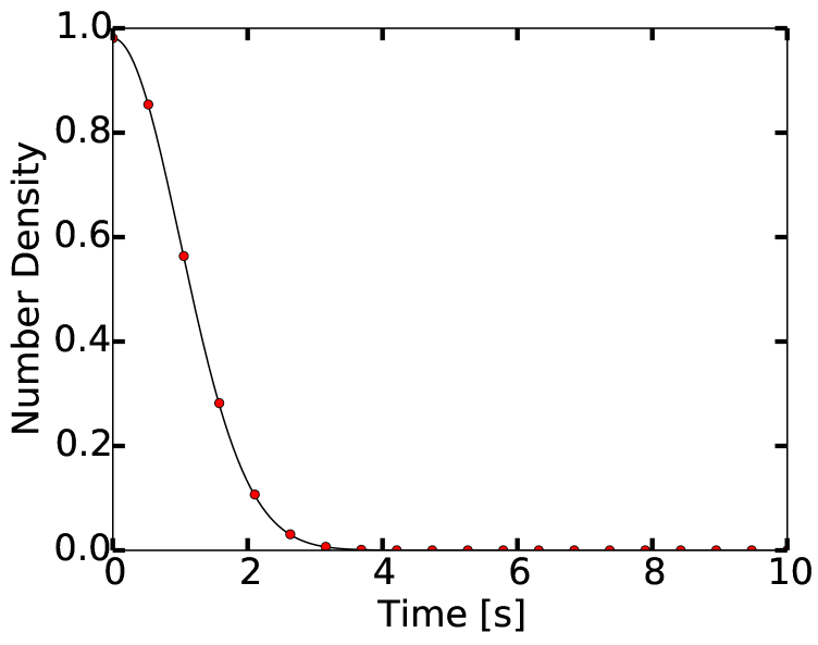
Figure 1: Number density (black) in cell 2 as a function of time for a free-streaming problem. SP1 basis functions with upwind flux are used on a $(N_{x},N_{v})=(64,64)$ grid. The red dots show the exact solution. At this resolution the numerical results are indistinguishable from the exact solution.

To test the ability of the algorithm to model this damping, a simulation is initialized with a Maxwellian with $v_{t}=1$ and $k=1$ on a domain $(x,v)\in[0,2\pi]\times[-6,6]$. The number density is computed and recorded in a specified cell. The simulation is run on a $(N_{x},N_{v})=(64,64)$ grid using SP1 basis functions. The number density measured in a cell is shown in Fig. 1. At this resolution the numerical results are indistinguishable from the exact solution.

The use of a discrete grid, however, combined with the lack of physical (or artificial) dissipation, leads to recurrence, i.e. the initial condition will recur after some finite time. This occurs as the phases of the discrete solution decohere temporarily leading to collisionless damping, however, after a finite time combine together again to recreate the initial conditions. A small amount of damping (via collisions or hyper-collisions), however, can easily control this recurrence even on a coarse grid.

4.3 Particle motion in specified potential

In this set of problems the potential $\phi(x)$ is held fixed in time and the distribution is evolved. These cases correspond to the motion of test particles in a specified potential. In each case the initial distribution is assumed to be a uniform Maxwellian

(43) $$f(x,v,0)=\frac{1}{\sqrt{2\pi v_{t}}}\exp(-v^{2}/2v_{t}^{2})$$

with $v_{t}=1$. If the potential has a well (a minima) then a fraction of the particles will be trapped and appear as rotating vortices in the distribution function plots. The bounce period for a particle with total energy $E$ (which is a constant of motion) in a well can be computed as

(44) $$T(E)=\sqrt{2m}\int_{x_{1}(E)}^{x_{2}(E)}\frac{dx}{\sqrt{E-\phi(x)}},$$

where $x_{1}$ and $x_{2}$ are the roots of the equation $\phi(x)=E$, i.e. the turning points at which the motion of the particle reverses. For finite $x_{1}$ and $x_{2}$ the motion is periodic. Note that for a non-singular distribution (like the Maxwellian) the bounce period need not be the same for all the particles. In this case an average period can be computed.

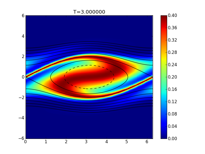
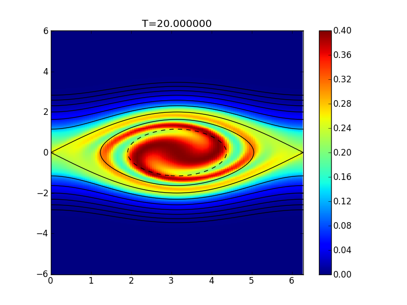
Figure 2: Distribution function at $t=3$ (left) and $t=20$ for flow in a $\cos(x)$ potential well. The black lines show contours of constant particle energy. A separatrix forms along the trapped–passing boundary.

For the first test we initialize $\phi(x)=\cos(x)$. Simulations were run with a SP1 scheme on a $64\times 128$ grid for $(x,v)\in[0,2\pi]\times[-6,6]$. In this potential the bounce period of a single particle depends on its initial energy, and the particles with lower total energy bounce faster. Snapshots of the distribution function are shown at a $t=3$ and $t=20$ in Fig. 2.

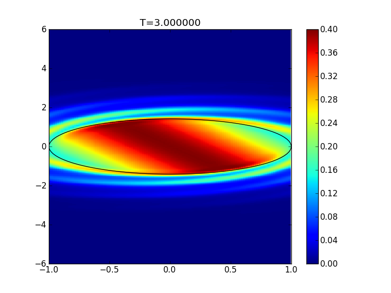
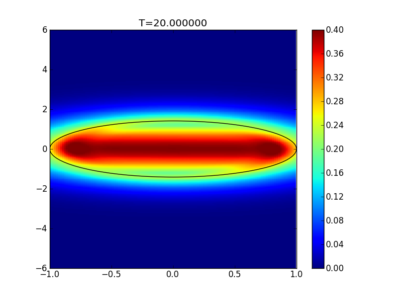
Figure 3: Distribution function at $t=3$ (left) and $t=20$ (right) for flow in a potential well. The black line shows the trapped–passing energy contour. Due to the quadratic potential $\phi(x)=x^{2}$, all particles inside the trapped region move with the same angular velocity in phase space, and the motion appears like rigid-body rotation.

In the second test we set $\phi(x)=x^{2}$. This quadratic potential corresponds to simple harmonic motion, and the bounce period of all trapped particles are the same and can be computed as $\pi\sqrt{2}\approx 4.443$. Also, as the bounce period for all trapped particles is the same, these will move “rigidly” in phase-space, i.e. the motion along contours of constant energy will occur with the same frequency. These features are clearly seen in the snapshots of the distribution function shown at $t=3$ and $t=20$ in Fig. 3.

4.3.1 Landau Damping

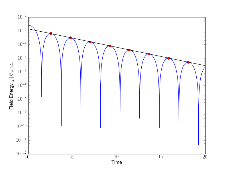
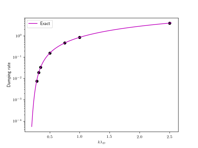
Figure 4: (Left) Field energy as a function of time for the linear Landau-damping problem with $k=0.5$ and $T_{e}=1.0$. The red dots represent the maxima in the field energy which are used to compute a linear least-squares fit. The slope of the black line gives the damping rate. (Right) Damping rate as a function of normalized Debye length. The black dots show the numerical damping rates compared to the exact results (magenta) computed from the dispersion relation.

Landau damping is the damping process of electrostatic plasma waves in a collisionless plasma. In this test the ability of the algorithm to capture the phenomena of Landau damping is shown. For this the electrons are initialized with a perturbed Maxwellian given by

(45) $$f(x,v,0)=\frac{1}{\sqrt{2\pi v_{t}^{2}}}\exp(-v^{2}/2v_{t}^{2})[1+\delta\cos(kx)],$$

where $v_{t}$ is the thermal velocity, $k$ is the wave number, and $\delta$ controls the perturbation. Periodic boundary conditions are imposed in the spatial direction and zero-flux conditions in the velocity direction. The ion density is set to $1$. The electrostatic field is determined from

(46) $$\frac{\partial^{2}\phi}{\partial x^{2}}=-\frac{\varrho_{c}}{\epsilon_{0}}=-\frac{1}{\epsilon_{0}}\left(1-\int fdv\right)$$

For all these tests $m=1$, $\epsilon_{0}=1$ and $\delta=0.01$. With these settings, the plasma frequency is $\omega_{pe}=1$ and the Debye length is $\lambda_{D}=\sqrt{T_{e}}$. The wave number is varied and the damping rates are computed as the slope of the least-squares line passing through successive maxima of the field energy. See Fig. 4 for details, which shows the field energy for the case $T_{e}=1.0$. Figure 4 also shows the numerical results compared to the exact values obtained from the dispersion relation for Langmuir waves.

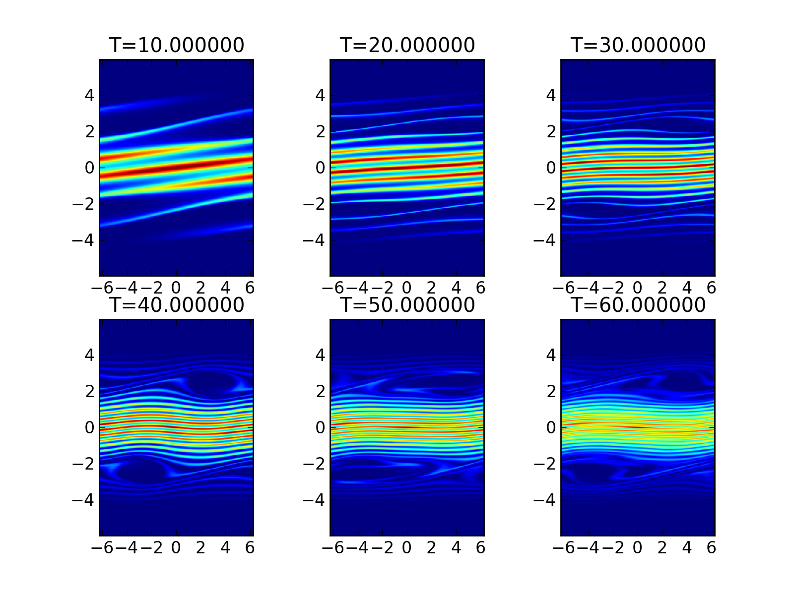
Figure 5: Distribution function at different times for the nonlinear Landau-damping problem. The initial perturbation undergoes shearing in phase space, leading to Landau damping from the phase mixing (see Fig. 4 for the damping rate). Starting at around $t=20$ the damping is halted due to particle trapping, finally leading to saturation. Phase-space holes are clearly visible.

If we increase the perturbation to $\delta=0.5$, the system is rapidly driven nonlinear. Other parameters are kept the same as for the linear Landau-damping problem with $k=0.5$ and $T_{e}=1.0$. In the nonlinear phase, the Landau damping eventually halts due to the formation of phase-space holes that lead to particle trapping that “shuts off” phase mixing (see Fig. 5).

Besides damping of electrostatic plasma waves, ion acoustic waves are also Landau damped. In this case we can assume that the electrons are a massless isothermal fluid. Hence we use, instead of the Poisson equation, the electron momentum equation to determine the potential. That is

(47) $$n_{i}(x)=n_{eo}\left(1+\frac{|e|\phi}{T_{e}}\right)$$

where, in this linear probem, $n_{eo}$ is the constant electron initial density and $T_{e}$ is the fixed electron temperature. This allows the determination of the potential once the ion number density is known. Note that this is an algebraic equation for $\phi$ and not a PDE. However, as the number density that appears in this is discontinuous (as the distribution function is discontinuous) this expression would mean that the potential $\phi$ is also discontinuous, violating the requirement for energy conservation. Hence, one realizes that this equation can only hold weakly, that is, one must construct the potential such that it belongs to the continuous subspace of the discontinuous basis: we must find $\phi_{h}$ such that

(48) $$\int\psi\left[n_{i}(x)-n_{eo}\left(1+\frac{|e|\phi_{h}}{T_{e}}\right)\right]\thinspace dx=0$$

for all continuous test functions $\psi(x)$. This is a global equation for $\phi$ (analogous to the Poisson equation which is also global) that results in a linear system needing inversion to compute the discrete potential.

We have performed tests for Landau damping of ion-acoustic waves in this approximation. The damping rates computed from our simulations (not shown) match the exact rates very accurately. In fact, the plot of damping with various values of $T_{i}/T_{e}$ looks identical to the right panel of Fig. 4 as the dispersion relation is exactly analogous to the case of Landau damping of electron oscillations. For a nonlinear application in gyrokinetics see[50] in which we studied the problem of heat-flux on divertor plates using a 1D gyrokinetic model, in which the field equation is local but the discrete potential needs to be determined using a non-local inversion along the magnetic field-line.

4.4 Incompressible Euler flow

In the final set of test problems we look at the incompressible Euler equations instead of the Vlasov–Poisson equations. The algorithms presented here are also applicable for this system as the incompressible Euler equations in 2D can be written in Hamiltonian form as described in the previous sections.

In the problem the simulation is initialized with two shear layers. The initially planar shear layers are perturbed slightly due to which they roll around each other, forming increasingly finer vortex-like features. The initial conditions for this problem are

(51) $$f(x,y,0)=\left\{\begin{array}[]{l l}\delta\cos(x)-\mathrm{sech}^{2}[(y-\pi/2)/\rho]/\rho\quad y\leq\pi\\ \delta\cos(x)+\mathrm{sech}^{2}[(3\pi/2-y)/\rho]/\rho\quad y>\pi\end{array}\right..$$

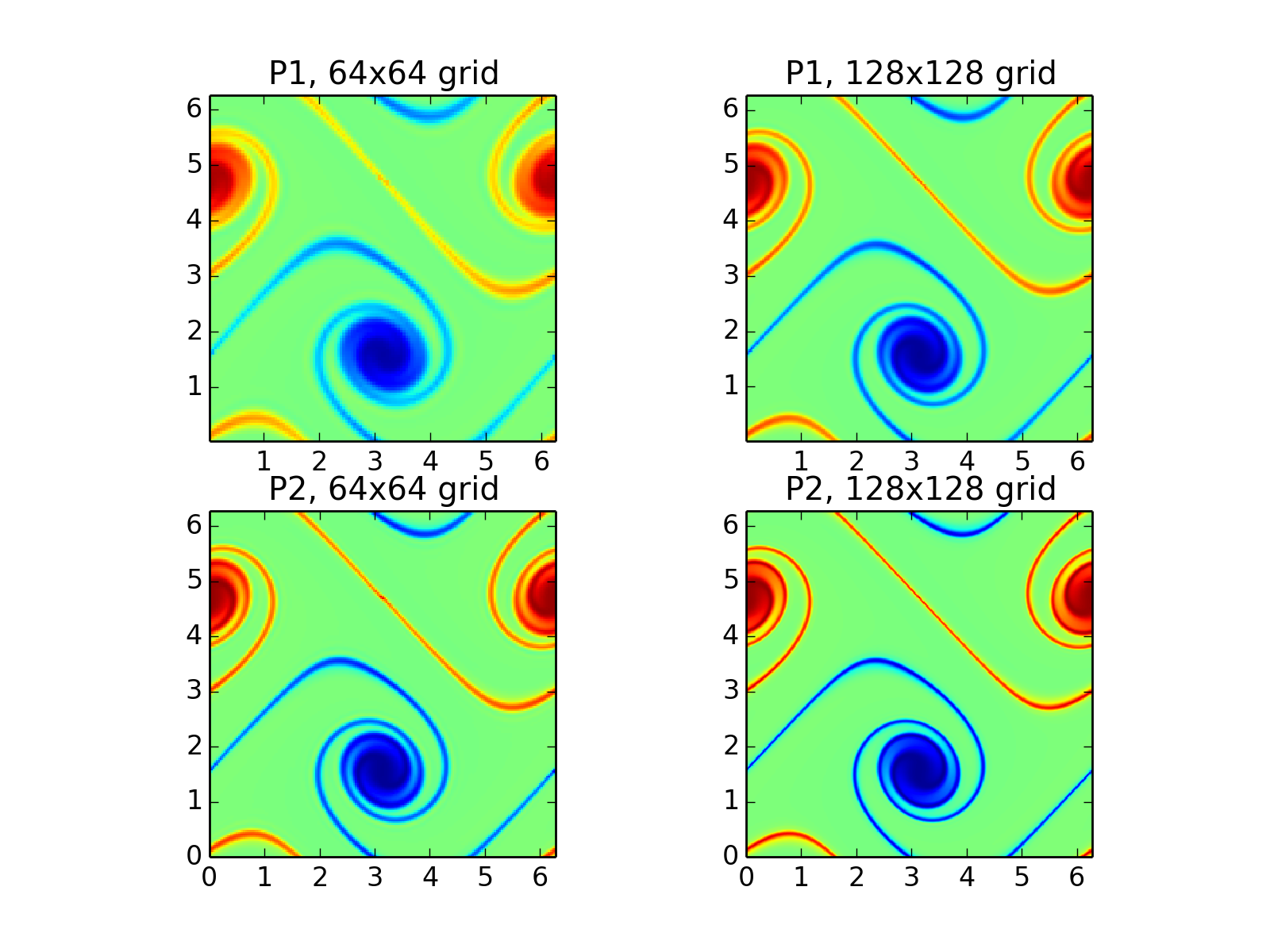
Figure 6: Double-shear-problem vorticity at t=8 with different grid resolutions and polynomial orders. Here, an upwind flux is used.

For the results shown, $\rho=\pi/15$ and $\delta=0.05$, and the problem is run to $t=8$. In the first set of simulations, an upwind flux was used with different grid sizes and spatial-order schemes to compute the solution. Figure 6 shows the results at the final time from these simulations. Recall that even though the energy is conserved with upwind fluxes, the enstrophy is not. To conserve enstrophy one can use central fluxes. With this the lack of energy and enstrophy conservation is solely due to the damping from the third-order Runge–Kutta time stepper used to advance the solution in time. As seen in Fig. 7 these errors reduce as $O(\Delta t^{3})$ as the time step is reduced.

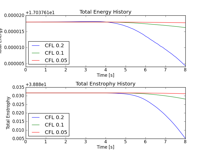
Figure 7: Total energy (top) and total enstrophy (bottom) history with different CFL numbers with central fluxes. Both energy and enstrophy errors asymptote to zero with the order of time-stepping scheme. The drop in energy is $1.36\times 10^{-5}$, $1.73\times 10^{-6}$ and $2.29\times 10^{-7}$ respectively, giving an order of $2.97$ and $2.91$. The drop in enstrophy is $2.66\times 10^{-2}$, $3.59\times 10^{-3}$ and $4.578\times 10^{-4}$ respectively, giving an order of $2.88$ and $2.97$.

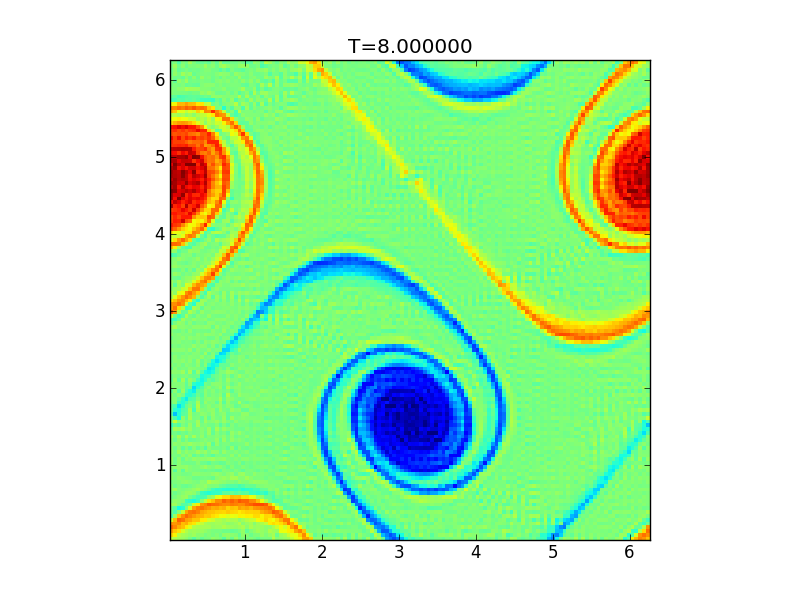
Figure 8: Vorticity at $t=8$ for double shear problem with central fluxes. Notice the significant phase errors in the solution as compared to the solution with the upwind fluxes (see Fig. 6). In general, a decaying enstrophy is desirable for stability.

Figure 8 shows that enstrophy conservation does not come for free: the lack of diffusion causes significant phase errors when the flow structures reach the grid scale. In general, a decaying enstrophy (or, more generally, a decaying $L_{2}$-norm of the solution) is desirable for stability.

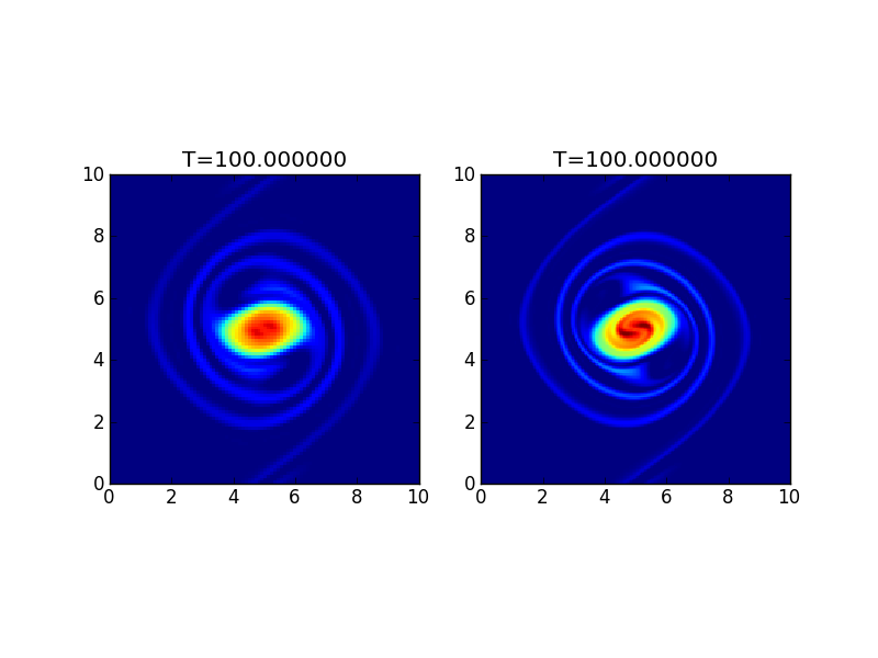
Figure 9: Vorticity for the vortex waltz problem with the second-order SP2 scheme. The left panel shows the solution with a $32\times 32$ grid, while the right panel shows the solution with a $64\times 64$ grid.

In the final problem the simulation was initialized with two Gaussian vortices which merge as they orbit around each other. The vorticity is initialized using the sum of two Gaussians given by

(52) $$f(x,y,0)=\omega_{1}(x,y)+\omega_{2}(x,y)$$

where

(53) $$\omega_{i}(x,y)=e^{-r_{i}^{2}/0.8}$$

where $r_{i}^{2}=(x-x_{i})^{2}+(y-y_{i})^{2}$ and $(x_{1},y_{1})=(3.5,5.0)$ and $(x_{2},y_{2})=(6.5,5.0)$. This is the “vortex-waltz” problem often used to benchmark schemes for the incompressible Euler equations. Figure 9 shows the solutions on $32\times 32$ and $64\times 64$ grids using the polynomial order 2 scheme with upwind fluxes. As for the double-shear problem, the energy and (not shown) are conserved to the order of the time-stepping scheme. Interestingly, the $p=2$ (SP2) scheme runs faster and gives higher accuracy on a coarser mesh than the $p=1$ (SP1) scheme. In general, this is a trend in all the simulations we have performed in which $p=2$ seems to be a “sweet spot” for accuracy and speed.

5 Conclusions

We have presented novel discontinuous Galerkin (DG) and continuous Galerkin (CG) schemes for the solution of a broad class of physical systems described by Hamiltonian evolution equations. These schemes conserve energy in the time-continuous limit, and the $L_{2}$ norm (and hence the entropy) when using central-fluxes to update the surface terms in the DG part of the scheme. They also conserve particles for arbitrary time step. Our energy conservation proof, rather surprisingly, is independent of upwinding (which adds dissipation in the DG update) while computing the distribution function. The physical reason for this is that updwinding is applied to the phase-space advection that happens to be perpendicular to the constant energy contours in phase-space. With updwinding, however, the $L_{2}$ norm decays monotonically, leading to a stable scheme with robust properties, providing some damping of barely-resolved grid-scale structures. We have applied these schemes to a broad variety of test problems and provided references to applications of our schemes to electrostatic and electromagnetic gyrokinetic equations, a system of considerable complexity that evolves in 5D phase-space. The scheme presented here does not ensure that the distribution function is positive, however. We have developed a novel scheme based on exponential reconstruction to ensure positivity but without changing the conservation properties of the scheme. This will be presented in a future publication. Overall, the scheme presented here has proved to be robust, accurate and, with novel choices of basis functions and automated code generation [26], very efficient. It forms the basis of much of our research into plasma turbulence in fusion machines [37, 49, 51, 52].

Appendix: Getting Gkeyll and reproducing the results. To allow interested readers to reproduce our results and also use Gkeyll for their applications, in this Appendix we provide instructions to get the code (in both binary and source format) as well as input files used here. Full installation instructions for Gkeyll are provided on the Gkeyll website (http://gkeyll.readthedocs.io). The code can be installed on Unix-like operating systems (including Mac OS and Windows using the Windows Subsystem for Linux) either by installing the pre-built binaries using the conda package manager (https://www.anaconda.com) or building the code via sources. The input files used here are under version control and can be obtained from the first author. Some are used as “regression tests” for the code. All tests can be run on a laptop.

References

- [1] A. Arakawa, Computational design for long-term numerical integration of the equations of fluid motion: Two-dimensional incompressible flow. part i, J. Comput. Phys., 1 (1966), pp. 119 – 143, https://doi.org/10.1016/0021-9991(66)90015-5.
- [2] D. N. Arnold and G. Awanou, The Serendipity Family of Finite Elements, Foundations of Computational Mathematics, 11 (2011), pp. 337–344.
- [3] B. Ayuso, J. Carrillo, and C.-W. Shu, Discontinuous galerkin methods for the one-dimensional vlasov-poisson system, Kinetic and Related Models, 4 (2011), pp. 955–989.
- [4] B. Ayuso de Dios, J. A. Carrillo, and C.-W. Shu, Discontinuous Galerkin methods for the multi-dimensional Vlasov–Poisson problem, Math. Models Methods Appl. Sci., 22 (2012), p. 1250042, https://doi.org/10.1142/S021820251250042X.
- [5] T. N. Bernard, E. L. Shi, K. W. Gentle, A. Hakim, G. W. Hammett, T. Stoltzfus-Dueck, and E. I. Taylor, Gyrokinetic continuum simulations of plasma turbulence in the Texas Helimak, Phys. Plasmas, 26 (2019), pp. 042301–12, https://doi.org/10.1063/1.5085457.
- [6] E. Bernsen, O. Bokhove, and J. J. van der Vegt, A (dis)continuous finite element model for generalized 2d vorticity dynamics, J. Comput. Phys., 211 (2006), pp. 719 – 747, https://doi.org/10.1016/j.jcp.2005.06.008.
- [7] C. Birdsall and A. B. Langdon, Plasma Physics Via Computer Simulation, Institute of Physics Publishing, 1990.
- [8] J. Candy, E. Belli, and R. Bravenec, A high-accuracy Eulerian gyrokinetic solver for collisional plasmas, J. Comput. Phys., 324 (2016), pp. 73–93, https://doi.org/10.1016/j.jcp.2016.07.039.
- [9] J. Candy and R. Waltz, An Eulerian gyrokinetic-Maxwell solver, J. Comput. Phys., 186 (2003), pp. 545–581, https://doi.org/10.1016/S0021-9991(03)00079-2.
- [10] J. Cary and A. Brizard, Hamiltonian theory of guiding-center motion, Reviews of Modern Physics, 81 (2009), pp. 693–738.
- [11] C. Z. Cheng and G. Knorr, The Integration of the Vlasov Equation in Configuration Space, J. Comput. Phys., 22 (1976), pp. 330–351, https://doi.org/10.1016/0021-9991(76)90053-X.
- [12] Y. Cheng, A. J. Christlieb, and X. Zhong, Energy-conserving discontinuous Galerkin methods for the Vlasov–Maxwell system, J. Comput. Phys., 279 (2014), pp. 145–173, https://doi.org/10.1016/j.jcp.2014.08.041.
- [13] Y. Cheng, I. Gamba, F. Li, and P. Morrison, Discontinuous Galerkin methods for the Vlasov–Maxwell equations, SIAM Journal on Numerical Analysis, 52 (2014), pp. 1017–1049, https://doi.org/10.1137/130915091.
- [14] Y. Cheng, I. M. Gamba, A. Majorana, and C.-W. Shu, A discontinuous Galerkin solver for Boltzmann-Poisson systems in nano devices, Computer Methods Appl. Mech. Engrg., 198 (2009), pp. 3130–3150.
- [15] Y. Cheng, I. M. Gamba, A. Majorana, and C.-W. Shu, A brief survey of the discontinuous Galerkin method for the Boltzmann-Poisson equations, SeMA J., 54 (2011), pp. 47–64. http://dx.doi.org/10.1007/BF03322587.
- [16] Y. Cheng, I. M. Gamba, and P. J. Morrison, Study of conservation and recurrence of Runge–Kutta discontinuous Galerkin schemes for Vlasov–Poisson systems, Journal of Scientific Computing, 56 (2013), pp. 319–349.
- [17] B. Cockburn and C.-W. Shu, The Runge–Kutta Discontinuous Galerkin Method for Conservation Laws V, J. Comput. Phys., 141 (1998), pp. 199–224.
- [18] B. Cockburn and C. W. Shu, Runge–Kutta discontinuous Galerkin methods for convection-dominated problems, Journal of Scientific Computing, 16 (2001), pp. 173–261.
- [19] D. Coulette and G. Manfredi, An Eulerian Vlasov code for plasma-wall interactions, Journal of Physics: Conference Series, 561 (2014), p. 012005, https://doi.org/10.1088/1742-6596/561/1/012005.
- [20] W. Dorland, F. Jenko, M. Kotschenreuther, and B. N. Rogers, Electron temperature gradient turbulence, Phys. Rev. Lett., 85 (2000), pp. 5579–5582, https://doi.org/10.1103/PhysRevLett.85.5579.
- [21] M. R. Dorr, P. Colella, M. A. Dorf, D. Ghosh, J. A. Hittinger, and P. O. Schwartz, High-order discretization of a gyrokinetic Vlasov model in edge plasma geometry, J. Comput. Phys., 373 (2018), pp. 605–630, https://doi.org/10.1016/j.jcp.2018.07.008.
- [22] L. Einkemmer and M. Wiesenberger, A conservative discontinuous Galerkin scheme for the 2D incompressible Navier–Stokes equations, Comput. Phys. Commun., 185 (2014), pp. 2865–2873, https://doi.org/10.1016/j.cpc.2014.07.007.
- [23] V. Grandgirard, J. Abiteboul, J. Bigot, T. Cartier-Michaud, N. Crouseilles, G. Dif-Pradalier, C. Ehrlacher, D. Esteve, X. Garbet, P. Ghendrih, G. Latu, M. Mehrenberger, C. Norscini, C. Passeron, F. Rozar, Y. Sarazin, E. Sonnendrücker, A. Strugarek, and D. Zarzoso, A 5D gyrokinetic full-f global semi-Lagrangian code for flux-driven ion turbulence simulations, Comput. Phys. Commun., 207 (2016), pp. 35–68, https://doi.org/10.1016/j.cpc.2016.05.007.
- [24] W. Guo and Y. Cheng, A sparse grid discontinuous Galerkin method for high-dimensional transport equations and its application to kinetic simulations, SIAM J. Sci. Comput., 38 (2016), pp. A3381–A3409, https://doi.org/10.1137/16M1060017.
- [25] A. Hakim, M. Francisquez, J. Juno, and G. W. Hammett, Conservative Discontinuous Galerkin Schemes for Nonlinear Fokker-Planck Collision Operators, arXiv.org, (2019), https://arxiv.org/abs/1903.08062.
- [26] A. Hakim and J. Juno, Generating a quadrature and matrix-free discontinuous galerkin algorithm for (plasma) kinetic equations, Journal of Computational Physics, Submitted (2019).
- [27] R. Heath, I. Gamba, P. Morrison, and C. Michler, A discontinuous Galerkin method for the Vlasov–Poisson system, J. Comput. Phys., 231 (2012), pp. 1140–1174, https://doi.org/10.1016/j.jcp.2011.09.020.
- [28] R. Hockney and J. Eastwood, Computer Simulation Using Particles, Taylor & Francis, 1989.
- [29] Y. Idomura, M. Ida, T. Kano, N. Aiba, and S. Tokuda, Conservative global gyrokinetic toroidal full-f five-dimensional Vlasov simulation, Comput. Phys. Commun., 179 (2008), pp. 391–403.
- [30] F. Jenko and W. Dorland, Nonlinear electromagnetic gyrokinetic simulations of tokamak plasmas, Plasma Phys. Control. Fusion, 43 (2001), pp. A141–A150, https://doi.org/10.1088/0741-3335/43/12a/310.
- [31] J. Juno, A. Hakim, J. TenBarge, E. Shi, and W. Dorland , Discontinuous Galerkin algorithms for fully kinetic plasmas, J. Comput. Phys., 353 (2018), pp. 110–147, https://doi.org/10.1016/j.jcp.2017.10.009.
- [32] K. Kormann, A semi-Lagrangian Vlasov solver in tensor train format, SIAM J. Sci. Comput., 37 (2015), pp. B613–B632, https://doi.org/10.1137/140971270.
- [33] K. Kormann, K. Reuter, and M. Rampp, A massively parallel semi-Lagrangian solver for the six-dimensional Vlasov–Poisson equation, Int. J. High Perform. Comput. Appl., 0 (0), p. 1094342019834644, https://doi.org/10.1177/1094342019834644.
- [34] D. K. Lilly, Introduction to “computational design for long-term numerical integration of the equations of fluid motion: Two-dimensional incompressible flow. part i”, J. Comput. Phys., 135 (1997), pp. 101–102, https://doi.org/10.1006/jcph.1997.5722.
- [35] J.-G. Liu and C.-W. Shu, A High-Order Discontinuous Galerkin Method for 2D Incompressible Flows, J. Comput. Phys., 160 (2000), pp. 577–596.
- [36] N. R. Mandell, W. Dorland, and M. Landreman, Laguerre-Hermite pseudo-spectral velocity formulation of gyrokinetics, J. Plasma Phys., 84 (2018), 905840108, p. 905840108, https://doi.org/10.1017/S0022377818000041.
- [37] N. R. Mandell, A. Hakim, G. W. Hammett, and M. Francisquez, Electromagnetic full- gyrokinetics in the tokamak edge with discontinuous Galerkin methods, J. Comput. Phys., (2019).
- [38] J. E. Marsden and A. Weinstein, The hamiltonian structure of the Maxwell-Vlasov equations, Physica D: Nonlinear Phenomena, 4 (1982), pp. 394–406, https://doi.org/10.1016/0167-2789(82)90043-4.
- [39] J. Morales-Escalante, I. M. Gamba, Y. Cheng, A. Majorana, C.-W. Shu, and J. Chelikowsky, Discontinuous Galerkin deterministic solvers for a boltzmann–poisson model of hot electron transport by averaged empirical pseudopotential band structures, Computer Methods in Applied Mechanics and Engineering, 321 (2017), pp. 209–234, https://doi.org/doi.org/10.1016/j.cma.2017.03.003.
- [40] P. J. Morrison, The Maxwell–Vlasov equations as a continuous hamiltonian system, Physics Letters A, 80 (1980), pp. 383 – 386, https://doi.org/10.1016/0375-9601(80)90776-8.
- [41] P. J. Morrison, A general theory for gauge-free lifting, Phys. Plasmas, 20 (2013), p. 012104, https://doi.org/10.1063/1.4774063.
- [42] P. J. Morrison and R. D. Hazeltine, Hamiltonian formulation of reduced magnetohydrodynamics, Phys. Fluids, 27 (1984), pp. 886–897, https://doi.org/10.1063/1.864718.
- [43] W. M. Nevins, G. W. Hammett, A. M. Dimits, W. Dorland, and D. E. Shumaker, Discrete particle noise in particle-in-cell simulations of plasma microturbulence, Phys. Plasmas, 12 (2005), p. 122305.
- [44] R. Numata, G. G. Howes, T. Tatsuno, M. Barnes, and W. Dorland, AstroGK: Astrophysical gyrokinetics code, J. Comput. Phys., 229 (2010), pp. 9347 – 9372, https://doi.org/10.1016/j.jcp.2010.09.006.
- [45] M. Nunami, T.-H. Watanabe, H. Sugama, and K. Tanaka, Gyrokinetic turbulent transport simulation of a high ion temperature plasma in large helical device experiment, Phys. Plasmas, 19 (2012), p. 042504, https://doi.org/10.1063/1.4704568.
- [46] M. Palmroth, U. Ganse, Y. Pfau-Kempf, M. Battarbee, L. Turc, T. Brito, M. Grandin, S. Hoilijoki, A. Sandroos, and S. von Alfthan, Vlasov methods in space physics and astrophysics, Living Reviews in Computational Astrophysics, 4 (2018), p. 1, https://doi.org/10.1007/s41115-018-0003-2.
- [47] A. Peeters, Y. Camenen, F. Casson, W. Hornsby, A. Snodin, D. Strintzi, and G. Szepesi, The nonlinear gyro-kinetic flux tube code GKW, Comput. Phys. Commun., 180 (2009), pp. 2650–2672, https://doi.org/10.1016/j.cpc.2009.07.001. 40 YEARS OF CPC: A celebratory issue focused on quality software for high performance, grid and novel computing architectures.
- [48] J. A. Rossmanith and D. C. Seal, A positivity-preserving high-order semi-Lagrangian discontinuous Galerkin scheme for the Vlasov-–Poisson equations, J. Comput. Phys., 230 (2011), pp. 6203–6232, https://doi.org/10.1016/j.jcp.2011.04.018.
- [49] E. L. Shi, Gyrokinetic Continuum Simulation of Turbulence in Open-Field-Line Plasmas, PhD thesis, Princeton University, 2017, https://arxiv.org/abs/1708.07283.
- [50] E. L. Shi, A. Hakim, and G. W. Hammett, A gyrokinetic one-dimensional scrape-off layer model of an edge-localized mode heat pulse, Physics of Plasmas, 22 (2015), p. 022504.
- [51] E. L. Shi, G. W. Hammett, T. Stoltzfus-Dueck, and A. Hakim, Gyrokinetic continuum simulation of turbulence in a straight open-field-line plasma, J. Plasma Phys, 83 (2017), https://doi.org/10.1017/S002237781700037X.
- [52] E. L. Shi, G. W. Hammett, T. Stoltzfus-Dueck, and A. Hakim, Full-f gyrokinetic simulation of turbulence in a helical open-field-line plasma, Physics of Plasmas, 26 (2019), p. 012307, https://doi.org/10.1063/1.5074179.
- [53] E. Sudarshan and N. Mukunda, Classical Dynamics: A Modern Perspective, Wiley, 1974.
- [54] Z. Tao, W. Guo, and Y. Cheng, Sparse grid discontinuous Galerkin methods for the vlasov-maxwell system, J. Comput. Phys.: X, 3 (2019), p. 100022, https://doi.org/0.1016/j.jcpx.2019.100022.
- [55] F. Valentini, P. Trávníček, F. Califano, P. Hellinger, and A. Mangeney, A hybrid-Vlasov model based on the current advance method for the simulation of collisionless magnetized plasma, J. Comput. Phys., 225 (2007), pp. 753–770, https://doi.org/10.1016/j.jcp.2007.01.001.
- [56] P. E. Vincent and A. Jameson, Facilitating the Adoption of Unstructured High-Order Methods Amongst a Wider Community of Fluid Dynamicists, Mathematical Modelling of Natural Phenomena, 6 (2011), pp. 97–140.
- [57] S. von Alfthan, D. Pokhotelov, Y. Kempf, S. Hoilijoki, I. Honkonen, A. Sandroos, and M. Palmroth, Vlasiator: First global hybrid-vlasov simulations of Earth’s foreshock and magnetosheath, J. Atmospheric Sol.-Terr. Phys., 120 (2014), pp. 24–35, https://doi.org/10.1016/j.jastp.2014.08.012.