Semi-Automatic Labeling for Deep Learning in Robotics

Abstract

In this paper, we propose Augmented Reality Semi-automatic labeling (ARS), a semi-automatic method which leverages on moving a 2D camera by means of a robot, proving precise camera tracking, and an augmented reality pen to define initial object bounding box, to create large labeled datasets with minimal human intervention. By removing the burden of generating annotated data from humans, we make the Deep Learning technique applied to computer vision, that typically requires very large datasets, truly automated and reliable. With the ARS pipeline we created effortlessly two novel datasets, one on electromechanical components (industrial scenario) and one on fruits (daily-living scenario), and trained robustly two state-of-the-art object detectors, based on convolutional neural networks, such as YOLO and SSD. With respect to conventional manual annotation of 1000 frames that takes us slightly more than 10 hours, the proposed approach based on ARS allows to annotate 9 sequences of about 35000 frames in less than one hour, with a gain factor of about 450. Moreover, both the precision and recall of object detection is increased by about 15% with respect to manual labelling. All our software is available as a ROS package in a public repository alongside with the novel annotated datasets.

Note to Practitioners— This paper was motivated by the lack of a simple and effective solution for the generation of datasets usable to train a data-driven model, such as a modern Deep Neural Network, so as to make them accessible in an industrial environment. Specifically, a deep learning robot guidance vision system would require such a large amount of manually labeled images that it would be too expensive and impractical for a real use case, where system reconfigurability is a fundamental requirement. With our system, on the other hand, especially in the field of industrial robotics, the cost of image labelling can be reduced, for the first time, to nearly zero, thus paving the way for self-reconfiguring systems with very high performance (as demonstrated by our experimental results). One of the limitations of this approach is the need to use a manual method for the detection of objects of interest in the preliminary stages of the pipeline (Augmented Reality Pen or Graphical Interface). A feasible extension, related to the field of collaborative robotics, could be to exploit the robot itself, manually moved by the user, even for this preliminary stage, so as to eliminate any source of inaccuracy.

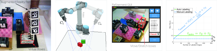
Figure 1: The system pipeline: 1) Draw virtual boxes around target objects; 2) Perform a scan acquiring camera poses (e.g. by a robot); 3) Refine virtual boxes; 4) Generate a training dataset. Therefore, with this approach it is possible to generate seamlessly an arbitrary number of self-labeled images without any human intervention. The right-most graph compares the time for manual labeling $\tau_{\text{manual}}$ (experimentally $\sim$100 images/hour) to that required by the proposed approach $\tau_{\text{auto}}$. The setup time $\tau_{\text{S}}$ is shared between the two modalities, $\tau_{\text{L}}$, instead, is the time required to label with the Augmented Reality Pen.

I Introduction

Many applications in modern robotics require a rich perception of the environment. The automatic detection of known objects, for instance, may help in scenarios like quality control, automated assembly, pick-and-place, bin-picking and so on. The specific task of object detection, as many others in computer vision, has witnessed dramatic advances in recent years due to the introduction of deep learning methods capable of recognizing many different object categories in real time [26, 11, 16]. Yet, these state-of-the-art methods mandate training on large datasets of images annotated with bounding boxes surrounding the objects of interest. The process of manually annotating the training images is time-consuming, tedious and prone to errors that may often lead to flimsy datasets or noisy annotations, especially when these are performed by non-professional users. Although a number of high-quality, large, multi-category training datasets are publicly available [17, 27, 3], they usually concern general classes (such e.g. person, car, cat, etc.) that may not suit the needs of a specific – industrial – task. In particular, robotic applications typically require detection of a relatively small set of specific object instances in cluttered and heavily occluded scenes captured from many different viewpoints, and with the sought objects possibly changing frequently overtime. In these settings, the richness and fickleness of the training dataset play a fundamental role to any deep learning solution. Indeed, handling a new object may easily require thousands of annotated images, which translates into tons of man-hours.

As at such large scale manual annotation turns out impractical and often inaccurate, we propose a user-friendly approach that allows to gather effortlessly and almost automatically huge datasets of annotated images in order to train state-of-the-art 2D Object Detectors based on deep learning like [26, 11, 16], or even 3D Pose Estimators like [14], [35], [25]. We start by acquiring a sequence of 2D images alongside with the camera pose in each frame. Based on this input information, our method deploys Augmented Reality techniques to enable the user to create easily the manual annotations for the first frame (or few ones) and then can deliver automatically accurate annotations for all the other frames of the sequence without any further human intervention. Hence, we dub our proposal ARS: Augmented Reality Semiautomatic-labeling. It is worth pointing out that the camera poses required by our method may be obtained in different manners, such as, e.g., by a monocular SLAM algorithm like [23, 7] or a motion capture system. Yet, as in this paper we mainly address robotic applications, we propose leveraging on a camera directly mounted on a robotic arm in an eye-on-hand configuration in order to gather tracked image sequences with high tracking accuracy, as also shown, e.g. , in [36, 5, 20]. We expect such an approach to become increasingly more practical and affordable with the advent of lightweight, but precise, collaborative robots, allowing the dataset creation directly on the application scenario, reducing in this way the gap, with regard to data distribution, between training and real conditions. We rely only on a plain 2D camera, which is cheap and does not set forth any restriction as long as objects are visible whereas a Stereo or RGB-D camera would have hindered flexibility, e.g. due to constraints on the minimum object-camera distance (and thus object size) or the inability to sense poorly textured or black surfaces. We developed a publicly available ROS package implementing all the tools described in this paper, which can be used to realize the ARS labelling pipeline starting from a video sequence with associated camera poses. Furthermore, we distribute all the datasets used throughout the experiments (see section IV), which enables reproducibility of the experimental results.

II Related work

A popular approach to speed-up creation of training datasets consists in the use of synthetic images rendered [18, 29, 21, 4] or even grabbed from realistic videogames [28, 13]. These techniques can deliver countless perfectly annotated images with human effort/time spent only to build synthetic scenes. However, obtaining a large dataset of photo realistic images usually comes at a cost as it may require hours of highly specialized human work to construct suitable synthetic environments plus many hours of computation on high-performance graphical hardware for rendering. In some practical settings, useful synthetic objects may be available beforehand in the form of CAD models although, indeed quite often, the textures may either be missing or look quite diverse with respect to the appearance of the actual objects.

Moreover, it is well known [21, 4] that training deep neural network by synthetic images does not yield satisfactory performance upon testing on real data due to the inherent difference between the ideal and real images, an issue often referred to as domain gap and calling for specific domain adaptation techniques, such as, e.g., fine-tuning the network by – fewer – manually annotated real images. Recent works [30, 37, 32, 2] focus on developing ad-hoc adaptation techniques to close the performance gap between training and test distribution. Unfortunately the performance achievable are still quite far from those obtainable training on real data or fine tuning on few annotated samples. Alternatively, to ameliorate the domain shift, [9] proposes an hybrid approach whereby an object detection system is trained on rendered views of synthetic 3D objects superimposed on real images; however, the blend between synthetic and real is far from perfect such that an additional fine-tuning on a real dataset is still needed. Differently, in this paper we propose a methodology to ease and speed-up the acquisition of large labeled datasets of real images which may be acquired directly in the deployment scenario, thereby avoiding any gap between the training and test domains.

Several approaches tailored to dataset creation have been proposed within the robotic research community: [15] proposes a system suitable for 3D face annotation, [36] proposes a semi-automatic technique to acquire a training dataset for object segmentation and [20] extends the idea to support object detection by leveraging on physical simulation to create realistic object arrangements. All this proposals require depth information from the sensor, and for the last two, realistic 3D models (e.g. textured CAD models). A similar solution is proposed in [24] and [33] where an environment is reconstructed by means of an RGB-D sensor and the labeling procedure is performed on the resulting 3D model. Conversely, our approach does not need any clue about he 3D shape of the object nor does it require depth information at training or test time. Moreover, our approach is the first technique usable with very small objects (as shown in [6]).

III Method description

Given a set of images, each equipped with the 6-DoF pose of the camera, and knowing the pose of the observed objects w.r.t. each vantage point, it is possible to project in each image some simplified representation of these items through augmented reality in order to generate automatically annotations (e.g. 2D bounding boxes, class labels, etc.) useful to train machine learning models. Subsection III-B describes formally the input data required by our proposed ARS labeling pipeline, which, as depicted in Figure 1, can be summarized in the following main steps:

1. Scene Setup (i.e. Arrange the objects randomly);

2. Outline virtual boxes around the target objects;

3. Scan the environment by a tracked camera;

4. Refine virtual boxes by visual analysis of the scan;

5. Generate automatically a training dataset.

ARS can be used to generate a dataset starting from scratch (i.e. following all the steps 0,1,2,3,4) or by exploiting archived material (i.e. following only steps 3 and 4, assuming the availability of an off-line camera tracker algorithm, like [23], to be applied to a recorded video sequence). The reminder of this section will describe in detail all the important steps of the labeling pipeline: Subsection III-B deals with the input data, Subsection III-C presents a way to define virtual boxes by an Augmented Reality Pen directly interacting with the physical environment, Subsection III-D addresses refining (or create a posteriori) virtual boxes around the objects and, finally, Subsection III-E describes the procedure used to generate annotated images. In Subsection III-A, we introduce the notation adopted throughout the rest of the paper.

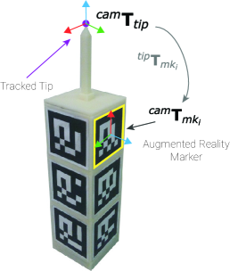
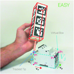
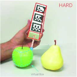
(a) ARP	(b) Drawing on geometrical object	(c) Drawing on rounded object

Figure 2: (a) The Augmented Reality Pen (ARP) used to draw virtual boxes. The pen features several Augmented Reality Markers with a known pose ${}^{tip}\mathbf{T}_{mk_{i}}$ w.r.t. the tip. (b) By tracking the tip position we can easily draw a virtual box around a target object by touching its edges. (c) Conversely, its not simple to draw a virtual box around a rounded object.

III-A Notation

We denote as ${}^{A}\mathbf{T}_{B}\in\mathbb{R}^{4\times 4}$ a 3D reference frame (briefly RF) $B$ expressed in the base $A$. So ${}^{0}\mathbf{T}_{cam}$ represents the RF linked to the camera in the $zero$ reference frame (i.e. the world RF). $m_{i}$ denotes a generic image and $b=\{x_{b},y_{b},w_{b},h_{b},c_{b}\}$ a square region (box) therein, with $(x_{b},y_{b})$ the coordinates of the center of $b$, $w_{b}$ and $h_{b}$ the width and height, respectively, and, optionally, $c_{b}\in\mathbb{Z}^{+}$ the class of the object contained in $b$.

III-B The input data

The input data to our labelling pipeline consist of two separate sets $\mathbb{F}$ and $\mathbb{I}$:

$$\begin{gathered}\mathbb{F}=\{F_{i}=\{^{0}C_{i},m_{i}\},i\in[0,...,n]\}\\ \mathbb{I}=\{V_{j}=\{^{0}\mathbf{T}_{j},s_{j},c_{j}\},j\in[0,...,k]\}\end{gathered}$$ (1)

$\mathbb{F}$ represent the acquired images (frames) $F_{i}=\{^{0}C_{i},m_{i}\}$ with ${}^{0}C_{i}$ being the camera matrix for image $m_{i}$. Each ${}^{0}C_{i}$ can be expressed as the multiplication of the intrinsics matrix $\hat{A}\in\mathbb{R}^{4\times 4}$ encoding camera specific parameters and the extrinsics matrix:

$${}^{0}\mathbf{T}_{cam_{i}}=\small{\begin{bmatrix}\mathbf{R}_{cam_{i}}&\mathbf{t}_{cam_{i}}\\ 0&1\end{bmatrix}}\in\mathbb{R}^{4\times 4}$$ (2)

encoding camera orientation ($\mathbf{R}_{cam_{i}}\in\mathbb{R}^{3\times 3}$) and position ($\mathbf{t}_{cam_{i}}\in\mathbb{R}^{3}$) with respect to the world frame.

$\mathbb{F}$ can be obtained using any method to track the camera movement, for example: a motion capture system, a SLAM based method like [23] or a camera mounted on a robotic arm in an eye-on-hand configuration. The $\mathbb{I}$ set, instead, corresponds to a collection of $k$ object instances present in the scenes. Each instance can be thought of as a 3D Virtual box, as shown in Figure 2(b-c), and can be expressed as a tuple $V_{j}=\{^{0}\mathbf{T}_{j},\mathbf{s}_{j},c_{j}\}$ with ${}^{0}\mathbf{T}_{j}$ the 6-DoF pose of the instance in the world reference frame, $\mathbf{s}_{j}\in\mathbb{R}^{3}$ the box dimensions and $c_{j}\in\mathbb{Z}^{+}$ its class. In the following we will cover different methodologies to collect a suitable $\mathbb{I}$ set.

III-C Online Labeling by the Augmented Reality Pen

To create $\mathbb{I}$ quickly and effortlessly, we developed the 3D printed artifact pictured in Figure 2, which resembles a pen covered with Augmented Reality Markers (in short: Markers [22]); we will refer to this device as to the ARP (Augmented Reality Pen). This tool can be used for labeling online object instances by interacting directly with the environment. Each Marker on the ARP has a known pose ${}^{tip}\mathbf{T}_{mk_{i}}$ w.r.t. the tip of the pen (the placement is CAD-driven). Using the OpenCV Marker Detector and the calibrated camera parameters we can estimate the pose of each of the markers, and consequently of the tip, w.r.t. the camera ${}^{cam}\mathbf{T}_{mk_{i}}$, then : $\small{}^{cam}\mathbf{T}_{tip}=^{cam}\mathbf{T}_{mk_{i}}\cdot(^{tip}\mathbf{T}_{mk_{i}})^{-1}$.

To achieve proper vertices estimation, the ARP is tracked exploiting multiple markers simultaneously, each of which contributes to refine the estimated tip position: by averaging those given by all the visible markers we can obtain a more accurate estimation of the real position. Accuracy therefore depends very much on the type of marker used, and has therefore not been dealt over in detail in this paper. As an indication, using this type of squared marker results in an error on the pose estimation proportional to the angle of inclination of the marker itself. A more detailed explanation of this approach, along with an accuracy analysis, is described in [12] and [34]. In particular, in [34] a dodecahedron (instead of our parallelepiped-shaped pen) is used to reduce the angle of view of visible markers, thus reducing the estimation error. As shown in Figure 2(b), as the ARP can be tracked while being used to – virtually – draw a box around an object, those 3D points can then be used to construct the corresponding tuple $V_{j}=\{^{0}\mathbf{T}_{j},s_{j},c_{j}\}$. Our approach requires only four specific points $p_{0},p_{1},p_{2},p_{3}$ placed as shown in Figure 2(b). Then, from those spatial positions we can obtain the corresponding components of $V_{j}$ as:

$$\begin{gathered}{}^{cam}\mathbf{T}_{j}=\begin{bmatrix}\mathbf{v}_{x}&\mathbf{v}_{z}\times\mathbf{v}_{x}&\mathbf{v}_{z}&\mathbf{p_{0}}\\ 0&0&0&1\end{bmatrix}\\ \\ \mathbf{v}_{z}=\frac{\textbullet\mathbf{p}_{1}-\mathbf{p}_{0}}{\left\|\mathbf{p}_{1}-\mathbf{p}_{0}\right\|},\mathbf{v}_{x}=\frac{\textbullet\mathbf{p}_{2}-\mathbf{p}_{1}}{\left\|\mathbf{p}_{2}-\mathbf{p}_{1}\right\|}\\ \\ s_{j}=\begin{bmatrix}s_{x}\\ s_{y}\\ s_{z}\end{bmatrix}=\begin{bmatrix}\left\|\mathbf{p}_{2}-\mathbf{p}_{1}\right\|\\ \left\|\mathbf{p}_{3}-\mathbf{p}_{2}\right\|\\ \left\|\mathbf{p}_{1}-\mathbf{p}_{0}\right\|\end{bmatrix}\end{gathered}$$ (3)

The class $c_{j}$ should instead be specified by the user. The Equation 3 specifies the RF of the virtual object ${}^{cam}\mathbf{T}_{j}$ referred to the camera RF; however, it can be easily transformed into the world RF by knowledge of the current camera pose ${}^{0}\mathbf{T}_{j}={{}^{0}}\mathbf{T}_{cam}\cdot{{}^{cam}}\mathbf{T}_{j}$.

By exploiting the ARP, a tight 3D bounding box can be easily created around box-like objects, such as in the case of electromechanical components, see Figure 2(b). However, this method will not work properly in case of arbitrarily shaped objects, such as the fruits depicted in Figure 2(c). To overcome this limitation, an off-line procedure to sketch $V_{j}$ by labeling a pair of frames picturing the same object from different vantage points has been developed, as reported in the following.

III-D Offline Labeling

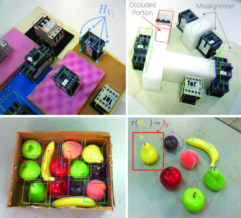
Figure 3: Four random frames acquired during the creation of our new dataset: the first row refers to the Industrial dataset and displays virtual boxes drawn by the ARP; the second row shows samples from the Fruits dataset with annotations created off-line by the technique described in Subsection III-D.

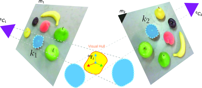
Figure 4: Graphical representation of the Visual Hull procedure used to build a virtual object from multiple 2D images.

In case of object with non-boxed shape, an offline procedure has been developed to increase the annotation accuracy with respect to what can be achieved by the ARP method previously described. The Fruits Dataset has been built by exploiting this off-line approach with good results, as shown in Figure 3. The offline procedure is based on a graphic interface through which the user can manually draw suitable masks around at least two different views of the object directly on the image frame. The complete procedure is detailed in the following.

As shown in Figure 3, upon acquisition of $\mathbb{F}$ and $\mathbb{I}$ it is quite straightforward to display frames from $\mathbb{F}$ with superimposed a 2D re-projection of the object instances defined in $\mathbb{I}$: each virtual object $V_{j}$ can be represented as a list of 3D points corresponding, in this specific case, to the eight vertices of the box. By arranging the vertices as columns of the matrix ${}^{0}P_{V_{j}}\in\mathbb{R}^{4\times 8}$ ($4$ rows are a result of the homogeneous coordinates conversion) and converting them in the $i_{\text{th}}$ camera RF, ${}^{cam}P_{V_{j}}=^{cam_{i}}\mathbf{T}_{0}\cdot{{}^{0}}P_{V_{j}}$, we can simply perform a 3D-to-2D re projection through:

$$\begin{bmatrix}\lambda H_{V_{j}}&1\end{bmatrix}^{\intercal}=\hat{A}\cdot{{}^{cam}}P_{V_{j}}$$ (4)

where $H_{V_{j}}$ is the set of corresponding 2D points and $\lambda$ the scale factor. This procedure is quite general and can be applied to any set of points (e.g. instead of virtual boxes we could have used virtual squares made by only 4 points if we are dealing with planar objects or arbitrary complex polygons for arbitrary shaped objects). Figure 3 shows many examples of reprojected virtual boxes $H_{V_{j}}$ each one being the 2D re projection of the virtual box $V_{j}$. However, as shown in Figure 3(top-right), the $H_{V_{j}}$ produced with the ARP tool can sometimes not be highly accurate due to several nuisances (e.g. the user hand-shake); therefore, we included in our software GUI a graphical tool that shows in augmented reality both the object and its bounding box from multiple points of view, as if the user was immersed in a 3D environment (see the third frame of Figure 1), by offering a browsable Mixed Reality scene [19].

This tool allows also to manually edit the bounding boxes, in order to correct the position, orientation and size of the virtual objects. Moreover, through the same GUI also a novel technique can be exploited to annotate the fruit dataset, in order to estimate the position of an object by analyzing two tracked frames (i.e. two rgb images of which I know the exact camera pose) without any initial guess. The aforementioned method consists simply in estimating a 3D virtual box (or a more complex 3D shape) by manually drawing its 2D re-projection on at least two frames, as depicted in Figure 4. Considering a pair of frames $F_{1},F_{2}$ we can draw two 2D masks $k_{1},k_{2}$ around the appointed object (the red apple in this case); knowing the two camera matrices ${}^{0}C_{1},^{0}C_{2}$ we can compute two view frustums which shall intersect – likely – in the center of mass of the real object producing what is generally called Visual Hull (VH) [1]. The pose of the new $V_{j}$ (i.e. ${}^{0}\mathbf{T}_{j}$) for the translational part can be computed easily using the center of mass of the VH, while for the rotational part we can choose the canonical identity matrix $I\in\mathbb{R}^{3\times 3}$ as a starting point. Finally, to complete the new $V_{j}$, we use the minimum bounding box algorithm, over the produced VH, to compute its dimensions $s_{j}$. It is important to note that a VH tends to be equal to the real 3D shape of the target object with the increase of the input frames labeled with the abovementioned technique, however the coarse $V_{j}$ created by this pipeline can be always manually refined using the already described interactive procedure.

III-E Genaration of the Training Data

The final step of the ARS labeling pipeline, once both $\mathbb{F},\mathbb{I}$ have been acquired and refined, is the creation of a training dataset suitable for modern machine learning models. In this work, as stated in the introduction, we mainly address the object detection task, which we will consider as an explanatory use case to show how to generate a training set. Our goal is to create a dataset consisting of images annotated with labeled 2D bounding boxes, $b_{j}$, surrounding each of the visible target objects. This information can be attained straightforwardly by simply reprojecting in each frame of $\mathbb{F}$ the 3D virtual objects in $\mathbb{I}$, i.e. $H_{V_{j}}$, and then computing a function to produce a squared bounding box $b_{j}$ from it. A graphical representation of the process is depicted in Figure 3 (bottom-right), where it is clear that $b_{j}=\tau(H_{V_{j}})$ is obtained through function $\tau(\cdot)$ (i.e. the minimum 2D bounding box), which indeed may be replaced by any custom function to obtain different kinds of labeled data (e.g. the convex hull).

IV Experimental evaluation

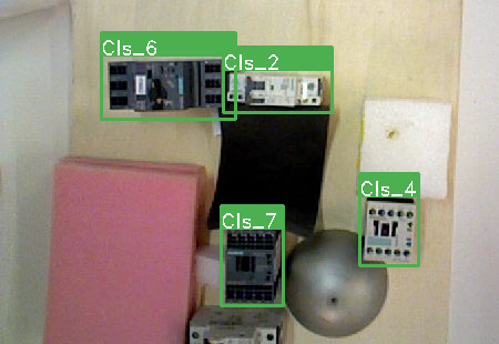
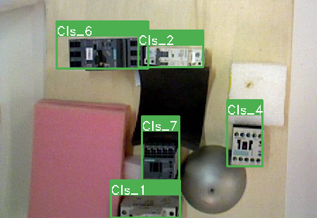
(a) Manual Industrial	(b) Auto Industrial

Figure 5: Samples from the dataset used for our experiments. The green rectangles display the annotated bounding boxes, the white text over each box is the class of that box. (a) Electromechanical components dataset annotated manually, (b) Electromechanical components dataset with auto-generated labels.

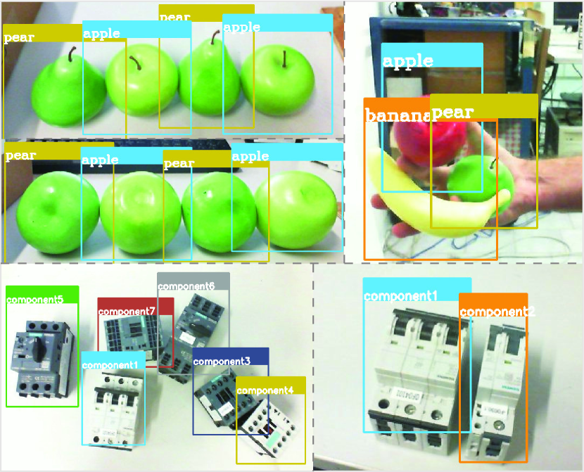
Figure 9: Detectors output (all correct) computed on images acquired with a usb webcam. The detector is able to distinguish apples and pears only looking at their lower side.

To validate the ARS pipeline we performed three sets of tests on two novel datasets that we are going to introduce in Subsection IV-A. In Subsection IV-B, we compare our automatic labeling procedure against a manual one. In Subsection IV-C, we show how our datasets can be used to train CNN based object detectors. In Subsection IV-D, we will compare monocular SLAM versus the use of a Robot for tracking the camera pose. Finally, in Subsection IV-E we introduce a new and interesting way of analyzing datasets, made possible only by our labeling approach. Some qualitative results are shown in Figure 9 as in the supplementary material, which also features a live demo of the ARS labeling procedure from scratch.

IV-A Datasets and evaluation metrics

To validate our proposal we choose as test beds two different detection tasks: one concerning recognition of 7 types of electromechanical components (Industrial), the other with 5 classes of fruits (Fruits); some samples from the two datasets are depicted in Figure 9. The first task concerns instance detection, as the items display low intra and inter class variability: the same components are seen across all the images from different vantage points, with different components looking remarkably similar. This kind of instance detection is used in the WIRES project (described in [10]) to implement a quality control and automated assembly systems for switchgear. The second task, instead, concerns object detection, as items show high intra and inter class variability: each fruit is quite different from the others, yet also fruits belonging to the same class can show quite different appearances, e.g. in our acquisition we have two kinds of apples and pears showing different peel colors. The produced fruits object detector can be used for a simple pick&place manipulation application. The first dataset is composed of 9 acquisition ($\sim 36000$ frames), the second by 8 shorter ones ($\sim 7500$ frames).

Both datasets were built by means of a camera mounted on an industrial manipulator, a COMAU Smart Six, with a position repeatability lesser than $0.05mm$. Using the industrial manipulator to move the camera we achieved a nearly perfect camera tracking, by computing the 6-DoF sensor pose through the robot kinematics, as to establish an upper bound for the labeling performance of ARS. We will show in Subsection IV-D how for less constrained applications, such us mobile robotics or home service robots, ARS could rely on a classical monocular SLAM pipeline for tracking the camera (although sacrificing some accuracy).

We chose one sequence from Industrial dataset and two from the Fruits dataset, manually annotating them, to be used as test sets for the trained object detectors, we will refer to them as Industrial_Test and Fruits_Test, respectively. The other sequences are randomly rearranged to create sets with increasing number of samples, each splitted in 80% train and 20% validation. We will refer to each one of such set as: $\langle$dataset name$\rangle$_$\langle$number of samples$\rangle$, e.g. Industrial_1000 identifies 1000 sample from the training sequences of Industrial that will be split into 800 training samples and 200 for validation. All datasets have been automatically annotated with ARS and for further tests we enriched Industrial_1000 with manual annotation as well. We will use a ”_M” suffix for a manually annotated dataset (e.g. Industrial_1000_M) and ”_A” suffix for annotation using ARS (e.g. Industrial_1000_A). Figure 1 shows a graphic comparison of the different efforts in human work hours needed to manually annotate a dataset (growing linearly with the number of required images) vs using ARS (constant once sequences are acquired and virtual boxes are created). For reference, factoring out the common acquisition time, the manual annotation of 1000 frames took us slightly more than 10 hours, while using ARS we were able to annotate all the 9 sequence of the Industrial dataset in less than an hour ($\sim 35000$ frames), with a gain of factor $\sim 450$.

To measure the detector performance we will use the standard object recognition metrics defined for the PASCAL VOC challenge [8]. Given a prediction $b_{j}^{p}$ and the corresponding ground truth box $b_{i}$, we consider $b_{j}$ correct if they have the same class and ${IOU(b_{j}^{p},b_{i})>IOU_{th}}$ with $IOU(\cdot)$ intersection over union of the boxes and $IOU_{th}$ a threshold parameters. Given the set of correct predictions we can measure: Precision,Recall and average intersection over union for correct predictions (avgIOU). Usually a detector produces quite a lot of $b_{j}^{p}$ each one associated with a certain confidence value $t_{j}^{p}\in[0,1]$, by thresholding the minimum confidence allowed we can tune the behaviour of the system. We represent the global performance with different confidence threshold using Precision/Recall curves and, concisely, with the mean average precision($mAP$), defined as the approximation of the area under the precision recall curve.

IV-B Annotation Study

In this section we want to test if the annotation obtained by ARS resemble what a human annotator would do. To verify this, we have compared the two sets of annotations, manual and auto-generated, by considering the first as the output of an ideal detector, while the second as ground truth annotations. Using $\small\text{IOU}_{th}=0.3$ we obtain the following performance: $\small\text{Precision}=98.49\%$, $\small\text{Recall}=95.02\%$ and $\text{avgIOU}=0.7$, i.e. comparing manual to automatic annotation the first set has fewer annotations (5% less Recall) and there exist some class misalignment (1.5% less Precision). To gain more insights on those differences, we visually examined the boxes obtained from the two sets of annotations and found out that the missing $1.5\%$ Precision can be mostly explained by class mistakes made by the human annotator during the labelling process, while ARS cannot assign any wrong label by construction. The $5\%$ missing recall is instead due to situations like that depicted in Figure 5(a-b), where the visible portion of an object (the bottom object Cls_1) is too small to allow the human annotator to recognize it. Finally, the relatively low $avgIOU$ highlights a key difference between ARS and a human annotator, the former always produces a box large enough to enclose the whole object as side effect of the re-projection of the virtual 3D box, while the latter usually encloses only the visible portion of the object (See the Figure 3 (top-right) image where a virtual box is drawn also where the object is occluded). As a result, the manual and auto annotations does not always have matching shapes, especially in cluttered environment, as it can be observed in Figure 5 (a-b). Nevertheless, as we will prove in the following paragraphs, the dataset labelled with ARS can effectively be used to train and validate any machine learning based object detector obtaining performance comparable with a manually annotated dataset of the same size, while also enabling an effortless training with many more images so as to create quite very robust object detectors.

IV-C Object Detector Test

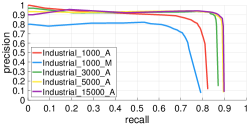
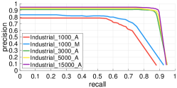
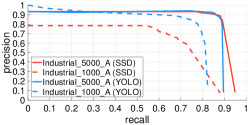
(a) YOLO	(b) SSD	(c) Comparison

Figure 6: Precision/Recall curves for the two type of detector trained on different subsets of the Industrial dataset. (a) and (b) report the results for YOLO and SSD respectively; (c) instead displays a comparison between them.

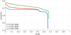
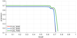
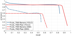
(a) YOLO	(b) SSD	(c) Class specific Comparison

Figure 7: Precision/Recall curves for the two type of detector trained on different subsets of the Fruits dataset. (a) and (b) report the results for YOLO and SSD respectively; (c) instead displays a comparison between SSD and YOLO over the best class (Banana) and the worst class (Pear) of the Fruits dataset.

	mAP (th=0.5)		avgIOU
Training set	YOLO	SSD	YOLO	SSD
Industrial_1000_M	0.589	0.619	0.7479	0.795
Industrial_1000_A	0.731	0.562	0.719	0.728
Industrial_3000_A	0.799	0.809	0.713	0.720
Industrial_5000_A	0.828	0.831	0.705	0.729
Industrial_15000_A	0.834	0.851	0.709	0.732

TABLE I: Mean average precision (mAP) and average intersection over union (avgIOU) on the Industrial_Test+ for YOLO and SSD trained using 5 different training sets with increasing number of images. Best result highlighted in bold.

	mAP (th=0.5)		mAP (th=0.3)		avgIOU
Training set	YOLO	SSD	YOLO	SSD	YOLO	SSD
Fruits_2500_A	0.438	0.468	0.895	0.888	0.710	0.744
Fruits_5000_A	0.440	0.465	0.894	0.889	0.6818	0.749
Fruits_7500_A	0.469	0.504	0.902	0.904	0.734	0.756

TABLE II: Mean average precision (mAP), at two different $IOU_{th}$, and average intersection over union (avgIOU) on Fruits_Test for YOLO and SSD trained using 3 different training sets with increasing number of images. ”A” suffix marks training sets with annotations produced by ARS, best result highlighted in bold.

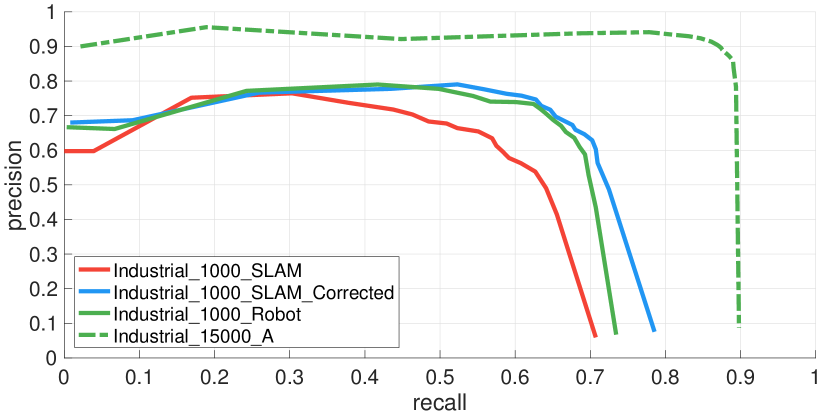
Figure 8: Precision/Recall curves for the YOLO detector trained on a subset of the Industrial dataset where the camera is also tracked with the Orb-Slam-v2 algorithm[23].

Once assessed that annotations obtained by ARS are comparable with manual ones, we test how effective is an object detector system trained on them. We choose as detectors YOLO [26] and SSD [11], using for both the original author’s implementation and public pre-trained networks as initial weights. The first tests concern the Industrial dataset where we defined a test bench of 126 images randomly picked from Industrial_Test plus 20 external smartphone pictures, all carefully manually annotated. We will call Industrial_Test+ this dataset. Thanks to the fast labelling obtained by ARS we were able to actually measure the performance boost related to the training set size using four different sets with increasing number of images, respectively Industrial_1000, 3000, 5000 and 15000. The samples for Industrial_1000 have both automatic and manual annotations, as to test if and how much the final detection performances change according to the label used.

Given the five different training sets, we trained both detectors on them for 100000 steps with batch_size=24 using the default hyperparameters recommended by the authors. The results are ten slightly different detectors that we tested on Industrial_Test+, we reported in Figure 6 the obtained precision/recall curves and in Table I the mAP and avgIOU. As expected, for both detectors the performance increases proportionally to the size of the training set used, e.g. +0.23 mAP gain between SSD trained on 1000 images and the best performing one trained on 15000; vouching the need for a method to ease and speed up the creation of huge training dataset. Inspecting the avgIOU obtained by the detectors we can see how the best performing methods are, unsurprisingly, the two trained on the manually annotated Industrial_1000_M. It is due to the fact the the testing images are manually annotated, so a manual label is better suited for an IOU score.

We repeated similar experiments on the Fruits dataset: we annotated all the eight sequences using ARS, then we produced three different training and validation sets with increasing number of samples and sequences, respectively Fruits_2500 (2 sequences), 5000 (4 sequences) and 7500 (6 sequences). As stated above, the remaining two sequences are used as the test bench for the detector creating a manual labelled test set of 1000 images (refereed as Fruits_Test). We tested the six different resulting detectors on Fruits_Test and report the result in Figure 7 and in Table II. Once again all the performance indexes increase alongside with the size of the training set, with best absolute performance obtained by SDD using the Fruits_7500 dataset. Figure 7(c) reports an intra-detector comparison between YOLO and SSD on the best and the worst class.

IV-D Comparision between visual SLAM and robot-based camera tracking

Aiming at the comparison between the ARS approach and what can be achieved through different kinds of camera trackers, the state-of-the-art monocular SLAM described in [23] has been exploited to track the camera on the acquired datasets, and the results are compared with the ones obtained through robot based camera tracking previously described. To this end, we use all the original Industrial training sequences to feed the visual SLAM algorithm, obtaining in this way a new version of the frame set in which the camera poses are estimated by tracking the visual features instead of measuring it through the robot.

Unfortunately, state of the art SLAM system featuring a pose optimization graph, can produce camera poses only for a subset of frames (i.e. the keyframes) much smaller than the original set.

In this specific case, the experimental compression ratio is about $1:30$, which results in reducing the dataset dimension to about 1000 images (starting from the 36000 of the Industrial dataset). We refer with Industrial 1000 SLAM to the direct outcome of the visual SLAM algorithm, while with Industrial 1000 Robot we refer to the corresponding frames in which the camera pose is estimated through the robot kinematics. Moreover, due to the known scaling factor problem of a monocular SLAM, the estimated camera poses may be slightly different from the real one, generating a non-perfect match with the original objects and, as a consequence, misaligned annotations.

However, by using ARS we manually corrected them with the procedure described in Subsection III-D producing an additional training set called Industrial 1000 SLAM Corrected. In Figure 8 we plot precision-recall curves obtained by YOLO trained on the three training sets. The performance of original SLAM procedure is worse than the corrected counterpart that is indeed comparable to the Robot version.

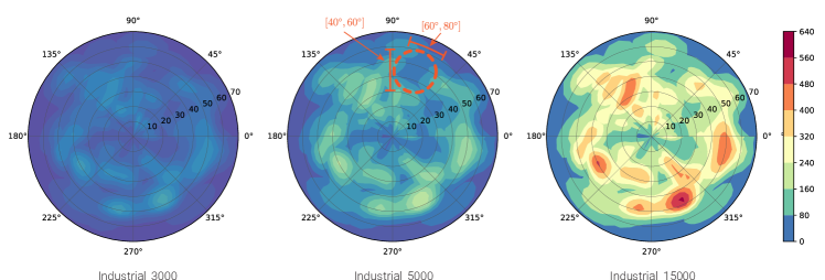
Figure 10: The Viewpoint Coverage computed for object of class 0 for the Industrial_3000/5000/15000 datasets. The ColorBar maps the color with the number of views voting for corresponding polar bin.

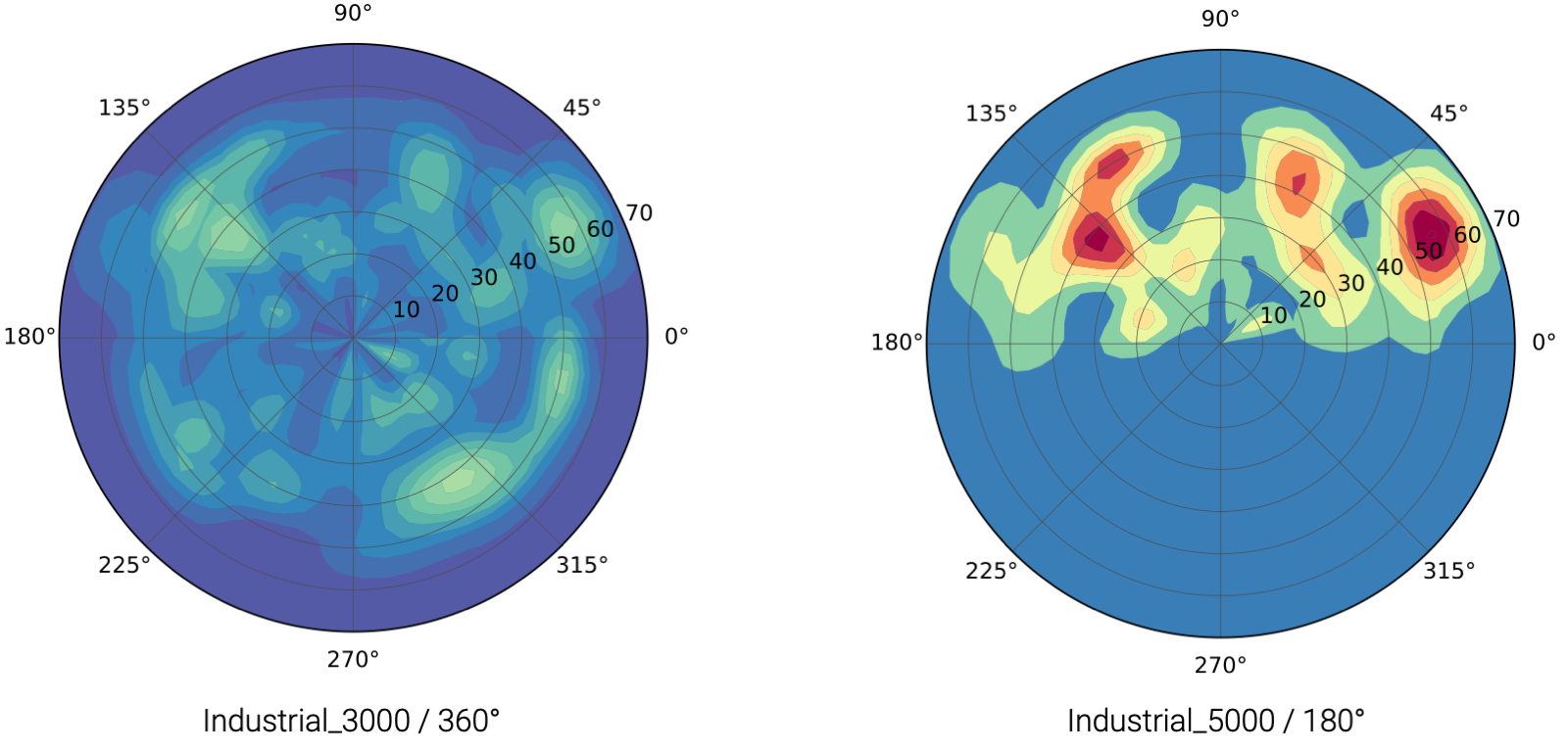
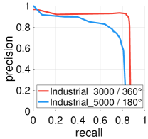
(a)	(b)

Figure 11: (a) Shows the VC over Industrial_3000 and Industrial_5000 with the latter filtered removing half the viewpoints. (b) Depicts the performance of an object detector trained on the two dataset, highlighting the importance of a full coverage at training time.

IV-E Viewpoint Coverage

All the results reported so far show that ARS is fast and effective for the dataset creation, however, it has one additional useful side effect: for each image in the dataset we know the position of the camera with respect to each object in the scene. Thus, for each virtual box $V_{j}=\{^{0}\mathbf{T}_{j},s_{j},c_{j}\}$ we can compute the position of the camera w.r.t. that object at the $i_{\text{th}}$ frame ${}^{j}\mathbf{T}_{cam_{i}}$. We can express the position of the camera in the object RF in polar coordinates ${}^{j}\mathbf{p}_{cam_{i}}=^{j}(r,\theta,\phi)_{cam_{i}}$ (i.e. radial, azimuthal, polar) and build a 2D histogram by aggregating $(\theta,\phi)$ into bins and counting the number of frames which contribute to that viewpoint. We dubbed this histogram the Viewpoints Coverage (VC) of an object in the training dataset. Figure 10 shows as heat map the histograms for object class $0$ on three of the Industrial training sets presented above, with hotter colors corresponding to higher coverage, i.e. to more frames acquired from that viewpoint. On the middle histogram of Figure 10 we highlighted with a dashed circle a region with low score, i.e. a viewpoint poorly covered in the training set and thus a potential flaw in the final detector when watching the object from that vantage point in a test image. Therefore the VC representation may be used during the creation of the dataset to guide the user (or a Robot), e.g. suggesting how to acquire new sequences carrying out better trajectories. To highlight the importance of having as much object coverage as possible we define two dataset Industrial_3000/360^∘ (featuring only 3000 images but covering all viewpoints) and Industrial_5000/180^∘ (featuring 5000 images but only covering half of the possible viewpoints) considering only object class $0$, with Figure 11(a) depicting the corresponding VCs. We use those as training set for YOLO and report in Figure 11(b) the resulting precision/recall curves for that object class. As expected, even featuring 2000 images more, Industrial_5000/180^∘ perform much worse due to having seen only a limited set of object appearances. In conclusion, with the Viewpoint Coverage analysis we demonstrate that methods like this are crucial to control the distribution of training data , which is much more relevant than the size of an uncontrolled dataset. In addition, in case of ARS deployed in a robotic scenario, the VC metrics could guide the robot to perform optimal trajectories to maximize the coverage of the viewpoints autonomously, or, in case of impossible trajectories, inform the user that there is a need to rearrange objects in the scene.

V Conclusion and Future Work

In this paper, we demonstrated how, by using robotic vision (i.e. robotics at the service of vision and vice versa), it is possible to create systems, such as the one here presented, that use the robot itself to learn. By exploiting the dexterity of the robot, a large number of viewpoints are automatically generated for each object (as depicted in Figure 10), to allow the neural networks to generalize well distilling a knowledge of them. Moreover, the possibility to generate self-annotated images without human intervention allows to effortlessly collect countless environmental variations (such as light or working table color changes) thus generating robust visual perception even in unstructured environments.

By the proposed approach, two novel datasets are effortlessly created, one on electromechanical components (industrial scenario) and one on fruits (daily-living scenario). From these datasets, two state-of-the-art object detectors based on convolutional neural networks, such as YOLO and SSD, are trained robustly. The proposed approach based on ARS allows to annotate 9 sequences of about 35000 frames in less than one hour, that compared to conventional manual annotation of 1000 frames that takes us slightly more than 10 hours, results in a gain factor of about 450 considering both the time saved and the dataset dimension. From the point of view of performance in the object detection, both the precision and recall is increased by about 15% with respect to manual labelling. The proposed approach allows to embed into robots novel and more performing perception and learning capabilities at the expense of a very limited human intervention. All the software generated to implement the proposed approach is available as a ROS package in a public repository alongside with the novel annotated datasets .

As a future extension of the proposed method, we will exploit the knowledge of the 6-DOF pose of objects with respect to the camera provided by the robot in each viewpoint to train more complex systems than a simple 2D detector. To this end, the approaches adopted to estimate the 3D position and orientation of objects from single 2D images reported in literature, see for example [14, 25, 31], will be trained with the output provided by the ARS pipeline. This approach will enable the realization of a fully automated self-learning BinPicking system.

Another ARS extension that we plan to explore concerns the use of out of the box augmented reality toolkit offered by nowadays mobile platforms (e.g. ARKit for iOS and ARCore for Android) in order to track the camera pose while acquiring video sequences. This extension would allow quick and easy creation of a training dataset by an off-the-shelf mobile device such as a smartphone or a tablet.

Daniele De Gregorio received the B.Sc. and M.Sc. degrees from the University of L’Aquila, Italy, in 2008 and 2012, respectively, and the Ph.D. degree in software engineering from the University of Bologna, Italy, in 2018. He is currently a Post-Doctoral Researcher with the University of Bologna. His research interests include robotics, computer vision, and deep learning.

Alessio Tonioni Received his PhD degree in Computer Science and Engineering from University of Bologna in 2019. Currently, he is a Post-doc researcher at Department of Computer Science and Engineering, University of Bologna. His research interest concerns machine learning for depth estimation and object detection.

Gianluca Palli received the Laurea and Ph.D. degrees in automation engineering from the University of Bologna, Bologna, Italy, in 2003 and 2007, respectively. He is currently an Associate Professor with the University of Bologna. He is an author or a co-author over 80 scientific papers presented at conferences or published in journals.

Luigi Di Stefano received the PhD degree in electronic engineering and computer science from the University of Bologna in 1994. He is currently a full professor at the Department of Computer Science and Engineering, University of Bologna, where he founded and leads the Computer Vision Laboratory (CVLab). His research interests include image processing, computer vision and machine/deep learning. He is the author of more than 150 papers and several patents. He has been scientific consultant for major companies in the fields of computer vision and machine learning. He is a member of the IEEE Computer Society and the IAPR-IC.

References

- [1] Baker, S., Kanade, T., et al.: Shape-from-silhouette across time part ii: Applications to human modeling and markerless motion tracking. International Journal of Computer Vision 63(3), 225–245 (2005)
- [2] Bousmalis, K., Irpan, A., Wohlhart, P., Bai, Y., Kelcey, M., Kalakrishnan, M., Downs, L., Ibarz, J., Pastor, P., Konolige, K., et al.: Using simulation and domain adaptation to improve efficiency of deep robotic grasping. arXiv preprint arXiv:1709.07857 (2017)
- [3] Calli, B., Singh, A., Bruce, J., Walsman, A., Konolige, K., Srinivasa, S., Abbeel, P., Dollar, A.M.: Yale-CMU-Berkeley dataset for robotic manipulation research. The International Journal of Robotics Research p. 027836491770071 (2017). DOI 10.1177/0278364917700714
- [4] Carlucci, F.M., Russo, P., Caputo, B.: A deep representation for depth images from synthetic data. In: Robotics and Automation (ICRA), 2017 IEEE International Conference on, pp. 1362–1369. IEEE (2017)
- [5] De Gregorio, D., Tombari, F., Di Stefano, L.: Robotfusion: Grasping with a robotic manipulator via multi-view reconstruction. In: Computer Vision–ECCV 2016 Workshops, pp. 634–647. Springer (2016)
- [6] De Gregorio, D., Zanella, R., Palli, G., Pirozzi, S., Melchiorri, C.: Integration of robotic vision and tactile sensing for wire-terminal insertion tasks. IEEE Transactions on Automation Science and Engineering (99), 1–14 (2018)
- [7] Engel, J., Schöps, T., Cremers, D.: Lsd-slam: Large-scale direct monocular slam. In: European Conference on Computer Vision, pp. 834–849. Springer (2014)
- [8] Everingham, M., Eslami, S.A., Van Gool, L., Williams, C.K., Winn, J., Zisserman, A.: The pascal visual object classes challenge: A retrospective. International journal of computer vision 111(1), 98–136 (2015)
- [9] Georgakis, G., Mousavian, A., Berg, A.C., Kosecka, J.: Synthesizing training data for object detection in indoor scenes. CoRR abs/1702.07836 (2017)
- [10] Gregorio, D.D., Zanella, R., Palli, G., Pirozzi, S., Melchiorri, C.: Integration of robotic vision and tactile sensing for wire-terminal insertion tasks. IEEE Transactions on Automation Science and Engineering pp. 1–14 (2018). DOI 10.1109/TASE.2018.2847222
- [11] Huang, J., Rathod, V., Sun, C., Zhu, M., Korattikara, A., Fathi, A., Fischer, I., Wojna, Z., Song, Y., Guadarrama, S., et al.: Speed/accuracy trade-offs for modern convolutional object detectors. In: Proceedings of the IEEE Conference on Computer Vision and Pattern Recognition (2017)
- [12] Jiawei, W., Li, Y., Tao, L., Yuan, Y.: Three-dimensional interactive pen based on augmented reality. In: Image Analysis and Signal Processing (IASP), 2010 International Conference on, pp. 7–11. IEEE (2010)
- [13] Johnson-Roberson, M., Barto, C., Mehta, R., Sridhar, S.N., Rosaen, K., Vasudevan, R.: Driving in the matrix: Can virtual worlds replace human-generated annotations for real world tasks? In: Robotics and Automation (ICRA), 2017 IEEE International Conference on, pp. 746–753. IEEE (2017)
- [14] Kehl, W., Manhardt, F., Tombari, F., Ilic, S., Navab, N.: Ssd-6d: Making rgb-based 3d detection and 6d pose estimation great again. In: The IEEE International Conference on Computer Vision (ICCV) (2017)
- [15] Kendrick, C., Tan, K., Williams, T., Yap, M.H.: An online tool for the annotation of 3d models. In: 2017 12th IEEE International Conference on Automatic Face Gesture Recognition (FG 2017), pp. 362–369 (2017). DOI 10.1109/FG.2017.52
- [16] Lin, T.Y., Goyal, P., Girshick, R., He, K., Dollar, P.: Focal loss for dense object detection. In: The IEEE International Conference on Computer Vision (ICCV) (2017)
- [17] Lin, T.Y., Maire, M., Belongie, S., Hays, J., Perona, P., Ramanan, D., Dollár, P., Zitnick, C.L.: Microsoft coco: Common objects in context. In: European conference on computer vision, pp. 740–755. Springer (2014)
- [18] Mayer, N., Ilg, E., Hausser, P., Fischer, P., Cremers, D., Dosovitskiy, A., Brox, T.: A large dataset to train convolutional networks for disparity, optical flow, and scene flow estimation. In: Proceedings of the IEEE Conference on Computer Vision and Pattern Recognition, pp. 4040–4048 (2016)
- [19] Milgram, P., Kishino, F.: A taxonomy of mixed reality visual displays. IEICE TRANSACTIONS on Information and Systems 77(12), 1321–1329 (1994)
- [20] Mitash, C., Bekris, K.E., Boularias, A.: A self-supervised learning system for object detection using physics simulation and multi-view pose estimation. In: Intelligent Robots and Systems (IROS), 2017 IEEE/RSJ International Conference on, pp. 545–551. IEEE (2017)
- [21] Movshovitz-Attias, Y., Kanade, T., Sheikh, Y.: How useful is photo-realistic rendering for visual learning? In: Computer Vision–ECCV 2016 Workshops, pp. 202–217. Springer (2016)
- [22] Munoz-Salinas, R.: Aruco: a minimal library for augmented reality applications based on opencv. Universidad de Córdoba (2012)
- [23] Mur-Artal, R., Tardós, J.D.: Orb-slam2: An open-source slam system for monocular, stereo, and rgb-d cameras. IEEE Transactions on Robotics 33(5), 1255–1262 (2017)
- [24] Nguyen, D.T., Hua, B.S., Yu, L.F., Yeung, S.K.: A robust 3d-2d interactive tool for scene segmentation and annotation. arXiv preprint arXiv:1610.05883 (2016)
- [25] Rad, M., Lepetit, V.: Bb8: A scalable, accurate, robust to partial occlusion method for predicting the 3d poses of challenging objects without using depth. In: International Conference on Computer Vision, vol. 1, p. 5 (2017)
- [26] Redmon, J., Farhadi, A.: Yolo9000: better, faster, stronger. In: Proceedings of the IEEE Conference on Computer Vision and Pattern Recognition (2017)
- [27] Rennie, C., Shome, R., Bekris, K.E., De Souza, A.F.: A dataset for improved rgbd-based object detection and pose estimation for warehouse pick-and-place. In: IEEE Robotics and Automation Letters, vol. 1, pp. 1179–1185. IEEE (2016)
- [28] Richter, S.R., Vineet, V., Roth, S., Koltun, V.: Playing for data: Ground truth from computer games. In: European Conference on Computer Vision, pp. 102–118. Springer (2016)
- [29] Ros, G., Sellart, L., Materzynska, J., Vazquez, D., Lopez, A.M.: The synthia dataset: A large collection of synthetic images for semantic segmentation of urban scenes. In: Proceedings of the IEEE Conference on Computer Vision and Pattern Recognition, pp. 3234–3243 (2016)
- [30] Shrivastava, A., Pfister, T., Tuzel, O., Susskind, J., Wang, W., Webb, R.: Learning from simulated and unsupervised images through adversarial training. In: Proceedings of the IEEE Conference on Computer Vision and Pattern Recognition (2017)
- [31] Sundermeyer, M., Marton, Z.C., Durner, M., Brucker, M., Triebel, R.: Implicit 3d orientation learning for 6d object detection from rgb images. In: European Conference on Computer Vision, pp. 712–729. Springer (2018)
- [32] Tzeng, E., Hoffman, J., Saenko, K., Darrell, T.: Adversarial discriminative domain adaptation. In: Computer Vision and Pattern Recognition (CVPR), vol. 1, p. 4 (2017)
- [33] Wong, Y.S., Chu, H.K., Mitra, N.J.: Smartannotator an interactive tool for annotating indoor rgbd images. In: Computer Graphics Forum, vol. 34, pp. 447–457. Wiley Online Library (2015)
- [34] Wu, P.C., Wang, R., Kin, K., Twigg, C., Han, S., Yang, M.H., Chien, S.Y.: Dodecapen: Accurate 6dof tracking of a passive stylus. In: Proceedings of the 30th Annual ACM Symposium on User Interface Software and Technology, pp. 365–374. ACM (2017)
- [35] Xiang, Y., Schmidt, T., Narayanan, V., Fox, D.: Posecnn: A convolutional neural network for 6d object pose estimation in cluttered scenes. arXiv preprint arXiv:1711.00199 (2017)
- [36] Zeng, A., Yu, K.T., Song, S., Suo, D., Walker, E., Rodriguez, A., Xiao, J.: Multi-view self-supervised deep learning for 6d pose estimation in the amazon picking challenge. In: Robotics and Automation (ICRA), 2017 IEEE International Conference on, pp. 1386–1383. IEEE (2017)
- [37] Zhang, Y., Qiu, Z., Yao, T., Liu, D., Mei, T.: Fully convolutional adaptation networks for semantic segmentation. In: Proceedings of the IEEE Conference on Computer Vision and Pattern Recognition, pp. 6810–6818 (2018)