Further tests of lepton flavour universality from the charged lepton energy distribution in $b\to c$ semileptonic decays: The case of $\Lambda_{b}\to\Lambda_{c}\ell\bar{\nu}_{\ell}$

Abstract

In a general framework, valid for any $H\to H^{\prime}\ell^{-}\bar{\nu}_{\ell}$ semileptonic decay, we analyze the $d^{2}\Gamma/(d\omega d\cos\theta_{\ell})$ and $d^{2}\Gamma/(d\omega dE_{\ell})$ distributions, with $\omega$ being the product of the hadron four-velocities, $\theta_{\ell}$ the angle made by the three-momenta of the charged lepton and the final hadron in the $W^{-}$ center of mass frame and $E_{\ell}$ the charged lepton energy in the decaying hadron rest frame. Within the Standard Model (SM), $d^{2}\Gamma/(d\omega dE_{\ell})\propto\left(c_{0}(\omega)+c_{1}(\omega)E_{\ell}/M+c_{2}(\omega)E^{2}_{\ell}/M^{2}\right)$, with $M$ the initial hadron mass. We find that $c_{2}(\omega)$ is independent of the lepton flavor and thus it is an ideal candidate to look for lepton flavor universality (LFU) violations. We also find a correlation between the $a_{2}(\omega)$ structure function, that governs the $(\cos\theta_{\ell})^{2}$ dependence of $d^{2}\Gamma/(d\omega d\cos\theta_{\ell})$, and $c_{2}(\omega)$. Apart from trivial kinematical and mass factors, the ratio of $a_{2}(\omega)/c_{2}(\omega)$ is a universal function that can be measured in any semileptonic decay, involving not only $b\to c$ transitions. These two SM predictions can be used as new tests in the present search for signatures of LFU violations. We also generalize the formalism to account for some new physics (NP) terms, and show that neither $c_{2}$ nor $a_{2}$ are modified by left and right scalar NP terms, being however sensitive to left and right vector corrections. We also find that the $a_{2}/c_{2}$ ratio is not modified by these latter NP contributions. Finally, and in order to illustrate our findings, we apply our general framework to the $\Lambda_{b}\to\Lambda_{c}\ell\bar{\nu}_{\ell}$ decay. We show that a measurement of $c_{2}$ (or $a_{2}$) for $\tau$ decay would not only be a direct measurement of the possible existence of NP, but it would also allow to distinguish from NP fits to $b\to c\tau\bar{\nu}_{\tau}$ anomalies in the meson sector, that otherwise give the same total and differential $d\Gamma/d\omega$ widths. We show that the same occurs for the other two terms, $c_{0}$ and $c_{1}$, that appear in $d^{2}\Gamma/(d\omega dE_{\ell})$, and for the $\cos\theta_{\ell}$ linear term of the angular distribution.

I Introduction

The discrepancies, between available data and the Standard Model (SM) predictions seen in semileptonic $B-$meson decays, point at the possible existence of new physics (NP), affecting to the third quark and lepton generations, responsible for lepton flavor universality (LFU) violations (for a recent review see Ref. Bifani et al. (2019)). Present average results for the ${\cal R}_{D^{(*)}}=\frac{\Gamma(B\to D^{(*)}\tau\bar{\nu}_{\tau})}{\Gamma(B\to D^{(*)}\ell\bar{\nu}_{\ell})}$ ratios ($\ell=e,\mu$), show a tension with the SM predictions at the 4.4 standard deviations ($\sigma$) level [Heavy Flavour Averaging Group (HFLAV) Amhis et al. (2017), using BaBar Lees et al. (2012, 2013), Belle Huschle et al. (2015); Sato et al. (2016); Hirose et al. (2017) and LHCb Aaij et al. (2015, 2018) data and SM predictions Aoki et al. (2017); Aaij et al. (2015); Bigi and Gambino (2016); Jaiswal et al. (2017) ]. New preliminary measurements by the Belle Collaboration Abdesselam et al. (2019) reduce however this tension with the SM predictions to 1.2$\sigma$. A general model-independent analysis of different $b\to c\ell\nu_{\ell}$ charged current (CC) transition operators has been addressed in Ref. Murgui et al. (2019) within an effective field theory approach. The main conclusion of this study is that the anomaly is still present and can be solved by NP, in agreement with previous works (see f.i. the pioneering work of Ref. Fajfer et al. (2012)).

This anomaly can be corroborated in $\Lambda_{b}\to\Lambda_{c}\ell\bar{\nu}_{\ell}$ decays, which are also governed by the $b\to c$ transition. The $\omega-$shape of the differential width for muons has been recently measured by the LHCb Collaboration Aaij et al. (2017), and there exist prospects Cerri et al. (2018) that the level of precision in the ${\cal R}_{\Lambda_{c}}=\frac{\Gamma(\Lambda_{b}\to\Lambda_{c}\tau\bar{\nu}_{\tau})}{\Gamma(\Lambda_{b}\to\Lambda_{c}\mu\bar{\nu}_{\mu})}$ ratio might reach that obtained for ${\cal R}_{D^{(*)}}$. The form factors relevant for this transition are strongly constrained by heavy quark spin symmetry (HQSS), since no subleading Isgur-Wise (IW) function occurs at order ${\cal O}(\Lambda_{QCD}/m_{b,c})$ and only two subleading functions enter at the next order Neubert (1994); Bernlochner et al. (2018). Precise results for the form factors were obtained in Ref. Detmold et al. (2015) using Lattice QCD (LQCD) with 2+1 flavors of dynamical domain-wall fermions. Leading and subleading HQSS IW functions are simultaneously fitted to LQCD results and LHCb data, and are used to accurately predict the ${\cal R}_{\Lambda_{c}}$ ratio in the SM Bernlochner et al. (2018). Therefore, this reaction is, from the theoretical point of view, as appropriate as the $B\to D^{(*)}$ processes for the study of $b\to c$ LFU violations. A sum rule relating ${\cal R}_{\Lambda_{c}}$ to ${\cal R}_{D^{(*)}}$, independent of any NP scenario up to small corrections, was found in Refs. Blanke et al. (2019a, b). There it is shown that ${\cal R}_{\Lambda_{c}}$ does not provide additional information on the Lorentz structure of NP but provides an important consistency check of the ${\cal R}_{D^{(*)}}$ measurements. The full four-differential angular distribution of the $\Lambda_{b}\to\Lambda_{c}(\to\Lambda^{0}\pi^{+})\ell^{-}\bar{\nu}_{\ell}$ decay has been recently studied in Ref. Böer et al. (2019) with the finding that the full set of angular observables analyzed is sensitive to more combinations of NP couplings than the ${\cal R}_{D^{(*)}}$ ratios. In this latter reference some discrepancies with the results of the previous study of Ref. Shivashankara et al. (2015) are pointed out. NP corrections to ${\cal R}_{\Lambda_{c}}$ have also been examined in other works Li et al. (2017); Datta et al. (2017); Bernlochner et al. (2019); Ray et al. (2019); Di Salvo et al. (2018); Murgui et al. (2019); Ferrillo et al. (2019). Some of them pay also attention to the double differential rate, $d^{2}\Gamma/(d\omega d\cos\theta_{\ell})$, in addition to ${\cal R}_{\Lambda_{c}}$ or the $\omega$ spectrum ($\omega$ being the product of the hadron four-velocities and $\theta_{\ell}$ the angle made by the three-momenta of the charged lepton and the final hadron in the center of mass (CM) of the two final leptons). Thus, forward-backward asymmetry has been calculated for this baryon decay Li et al. (2017); Datta et al. (2017); Bernlochner et al. (2019); Ray et al. (2019), while the full CM charged lepton angular dependence has also been analyzed for $B-$meson reactions, see f.i. Fajfer et al. (2012); Murgui et al. (2019). However, to our knowledge, the charged lepton energy ($E_{\ell}$) distribution in the decaying hadron rest frame has never been considered neither for $\Lambda_{b}\to\Lambda_{c}$ nor $B\to D^{(*)}$ semileptonic decays.

Finally, we should also mention that the $\Lambda_{b}\to\Lambda_{c}\ell\bar{\nu}_{\ell}$ decay provides an alternative method to determine the Cabibbo-Kobayashi-Maskawa matrix element $|V_{cb}|$ and to study the unitarity triangle within the SM.

In this work we introduce a general framework to study any baryon/meson semileptonic decay for unpolarized hadrons, though we refer explicitly here to those induced by the $b\to c$ transition. Within this scheme we find general expressions for the $d^{2}\Gamma/(d\omega d\cos\theta_{\ell})$ and $d^{2}\Gamma/(d\omega dE_{\ell})$ differential decay widths (see below), each of them expressible in terms of three different structure functions (SFs). Proceeding in this way, we have uncovered two new observables that can be measured and used as model independent tests for LFU violation analyses. This is discussed in next section, and it constitutes the most relevant result of this work. Indeed, we identify two contributions, one in the $E_{\ell}$ spectrum and a second one in the $\cos\theta_{\ell}$ distribution, which are independent of the lepton flavor in the SM. They provide novel, model-independent and clean tests of LFU. Moreover, we show that the ratio of both of them within the SM should be a universal function, which could be measured in all type of hadron (baryon or meson) semileptonic decays governed by CC $c\to s$, $c\to d$, $s\to u$, $b\to u$ transitions. This charged lepton energy-angle correlation should be experimentally accessible and, if violated, it would be a clear indication of NP, also eliminating some possible Lorentz structures for the new terms as we will discuss.

We also generalize the formalism to account for left and right scalar and vector NP contributions using the scheme of Ref. Murgui et al. (2019).

To illustrate our findings, we will apply the general framework to the analysis of the $\Lambda_{b}\to\Lambda_{c}$ decay. Using the state of the art LQCD form factors of Ref. Detmold et al. (2015), we evaluate the six SM SFs and the $d\Gamma/d\omega$ differential rate. For the case of a final $\tau$ lepton we give explicitly the contributions coming from positive and negative helicities measured, both in the CM of the $W^{-}$ boson and in the $\Lambda_{b}$ rest frame (LAB). As mentioned above, the relevance of the LAB lepton energy spectrum for LFU violation has never been studied for $\Lambda_{b}$ or for $B$ decays. Indeed, we also discuss how some features of that spectrum can be used to distinguish between different NP scenarios that otherwise lead to the same total and differential semileptonic decay widths.

II Decay Width

We consider the semileptonic decay of a bottomed hadron ($H_{b}$) into a charmed one ($H_{c}$) and $\ell\bar{\nu}_{\ell}$, driven by the CC $b\to c$ transition. In the SM, the differential decay width for massless neutrinos reads Tanabashi et al. (2018),

$$\frac{d^{2}\Gamma}{d\omega ds_{13}}=\frac{G^{2}_{F}|V_{cb}|^{2}M^{\prime 2}}{(2\pi)^{3}M}L^{\mu\nu}(k,k^{\prime})W_{\mu\nu}(p,q)$$ (1)

with $G_{F}=1.166\times 10^{-5}$ GeV^-2 the Fermi coupling constant, $M$ ($M^{\prime}$) the mass of the initial (final) hadron and $W$ and $L$, the hadron and lepton tensors. The latter one, after summing over all lepton polarizations is given by ($\epsilon_{0123}=+1$)

$$L_{\mu\nu}(k,k^{\prime})=k^{\prime}_{\mu}k_{\nu}+k_{\mu}k^{\prime}_{\nu}-g_{\mu\nu}k\cdot k^{\prime}+i\epsilon_{\mu\nu\alpha\beta}k^{\prime\alpha}k^{\beta}\,,$$ (2)

with $k^{\prime}$ ($k$) the outgoing charged lepton (neutrino) four-momentum. In addition, the product of the two hadron four velocities $\omega$ and $q^{2}=(k+k^{\prime})^{2}$ are related via $q^{2}=M^{2}+M^{\prime 2}-2MM^{\prime}\omega$ and $s_{13}=(p-k)^{2}$, with $p$ the four momentum of the decaying $H_{b}$ particle. Finally, the dimensionless hadron tensor is constructed from the non-leptonic CC vertex $j^{\mu}_{cc}=\bar{c}(0)\gamma^{\mu}(1-\gamma_{5})b(0)$ as

$$W^{\mu\nu}(p,q)=\overline{\sum}\langle H_{c};p^{\prime}|j_{cc}^{\mu}|H_{b};p\rangle\langle H_{c};p^{\prime}|j_{cc}^{\nu}|H_{b};p\rangle^{*}$$ (3)

with $p^{\prime}=p-q$. The sum is done over initial (averaged) and final hadron spins, and the states are normalized as $\langle\vec{p},r|\vec{p}\,^{\prime},s\rangle=(2\pi)^{3}(E/M)\delta^{3}(\vec{p}-\vec{p}\,^{\prime})\delta_{rs}$, with $r,s$ spin indexes. Lorentz covariance leads to the general decomposition

$$W^{\mu\nu}(p,q) = -g^{\mu\nu}W_{1}+\frac{p^{\mu}p^{\nu}}{M^{2}}W_{2}+i\epsilon^{\mu\nu\alpha\beta}p_{\alpha}q_{\beta}\frac{W_{3}}{2M^{2}}$$ (4)

$$+ \frac{q^{\mu}q^{\nu}}{M^{2}}W_{4}+\dfrac{p^{\mu}q^{\nu}+p^{\nu}q^{\mu}}{2M^{2}}W_{5}$$

actually valid for any $H\to H^{\prime}$ CC transition with unpolarized hadrons. The $W_{i}$ SFs are scalar functions of $q^{2}$ or equivalently of $\omega$. The double differential decay width can be rewritten introducing the angle ($\theta_{\ell}$) made by the charged lepton ($\ell$) and the final hadron ($H_{c}$) in the $W^{-}$boson CM frame as

$$\frac{d^{2}\Gamma}{d\omega d\cos\theta_{\ell}} = \frac{G^{2}_{F}|V_{cb}|^{2}M^{\prime 3}M^{2}}{16\pi^{3}}\sqrt{\omega^{2}-1}\left(1-\frac{m_{\ell}^{2}}{q^{2}}\right)^{2}A(\theta_{\ell})$$

$$A(\theta_{\ell}) = a_{0}(\omega)+a_{1}(\omega)\cos\theta_{\ell}+a_{2}(\omega)\cos^{2}\theta_{\ell}$$ (5)

$$a_{0} = 2\frac{q^{2}}{M^{2}}W_{1}+\frac{M^{\prime 2}}{M^{2}}(\omega^{2}-1)W_{2}$$

$$+ \frac{m^{2}_{\ell}}{q^{2}}\left(\frac{M_{\omega}^{2}}{M^{2}}W_{2}+\frac{q^{4}}{M^{4}}W_{4}+\frac{q^{2}M_{\omega}}{M^{3}}W_{5}\right)$$

$$a_{1} = -\frac{q^{2}M^{\prime}}{M^{3}}\sqrt{\omega^{2}-1}\,W_{3}$$

$$+ \sqrt{\omega^{2}-1}\,\frac{m^{2}_{\ell}}{q^{2}}\frac{M^{\prime}}{M}\left(2\frac{M_{\omega}}{M}W_{2}+\frac{q^{2}}{M^{2}}W_{5}\right)$$

$$a_{2} = -\frac{M^{\prime 2}}{M^{2}}(\omega^{2}-1)\left(1-\frac{m^{2}_{\ell}}{q^{2}}\right)W_{2}$$ (6)

with $M_{\omega}=(M-M^{\prime}\omega)$ and $m_{\ell}$ the mass of the charged lepton. The variable $\omega$ varies from 1 to $\omega_{\rm max}=(M^{2}+M^{\prime 2}-m^{2}_{\ell})/(2MM^{\prime})$ and $\cos\theta_{\ell}$ between $-1$ and 1. The terms proportional to $m_{\ell}^{2}$ in each of the coefficients $a_{i=0,1,2}$ account for the contributions from positive helicity of the outgoing $\ell$. This follows from the expression of the lepton tensor for a charged lepton with well defined helicity ($h=\pm 1$),

$$L_{\mu\nu}(h) = \frac{L_{\mu\nu}}{2}-\frac{h}{2}s^{\alpha}$$ (7)

$$\times \left(k_{\mu}g_{\nu\alpha}+k_{\nu}g_{\mu\alpha}-k_{\alpha}g_{\mu\nu}+i\epsilon_{\mu\nu\alpha\beta}k^{\beta}\right)\,,$$

where $s^{\alpha}=(|\vec{k}^{\prime}|,k^{\prime 0}\hat{k}^{\prime})$ and $\hat{k}^{\prime}=\vec{k}^{\prime}/|\vec{k}^{\prime}|$.

We are also interested in the double differential decay width with respect to $\omega$ and the energy ($E_{\ell}$) of the charged lepton in the LAB frame

$$\frac{d^{2}\Gamma}{d\omega dE_{\ell}} = \frac{G^{2}_{F}|V_{cb}|^{2}M^{\prime 2}M^{2}}{8\pi^{3}}\left[c_{0}(\omega)+c_{1}(\omega)\frac{E_{\ell}}{M}+c_{2}(\omega)\frac{E^{2}_{\ell}}{M^{2}}\right]$$

$$c_{0} = \frac{q^{2}}{M^{2}}\left(2W_{1}-W_{2}-\frac{M_{\omega}}{M}W_{3}\right)$$

$$+ \frac{m^{2}_{\ell}}{M^{2}}\left(-2W_{1}+W_{2}+\frac{M_{\omega}}{M}(2W_{4}+2W_{5}-W_{3})\right.$$

$$- \left.\frac{M^{2}-M^{\prime 2}+m^{2}_{\ell}}{M^{2}}W_{4}\right)$$

$$c_{1} = 2\left(2\frac{M_{\omega}}{M}W_{2}+\frac{q^{2}}{M^{2}}W_{3}-\frac{m_{\ell}^{2}}{M^{2}}W_{5}\right)$$

$$c_{2} = -4W_{2}$$ (8)

with $E_{\ell}\in[E_{\ell}^{-},E_{\ell}^{+}]$ and

$$E_{\ell}^{\pm}=\frac{M_{\omega}(q^{2}+m^{2}_{\ell})\pm M^{\prime}\sqrt{\omega^{2}-1}(q^{2}-{m^{2}_{\ell}})}{2q^{2}}$$ (9)

The relevance of this distribution is in the fact that within the SM, and up to small electroweak corrections, the $c_{2}(\omega)$ SF does not depend on the lepton mass. Therefore, this function determined in $\ell=e,\mu$ decays should be the same as that seen in $\tau$ decays. This is a clear test for LFU in all type of semileptonic $b\to c$ decays that to our knowledge has not been considered so far. A similar comment holds for $a_{2}(\omega)$ entering in the CM angular distribution of Eq. (5), after accounting for the trivial $(1-m_{\ell}^{2}/q^{2})$ kinematical factor. Furthermore, the ratio

$$\frac{M^{2}}{M^{\prime 2}}\frac{a_{2}(\omega)}{(1-m_{\ell}^{2}/q^{2})c_{2}(\omega)}=(\omega^{2}-1)/4$$ (10)

is a universal function that should be found in all type of $q\to q^{\prime}\ell\bar{\nu}_{\ell}$ transitions, since in that ratio the SF $W_{2}$ cancels out. This is a test of the predictions of the SM and, in principle, this ratio can be measured in any semileptonic decay: $D\to\bar{K}$, $D\to\pi$, $D\to\bar{K}^{*}$, $D\to\rho$, $\bar{K}\to\pi$, $\bar{B}_{s}\to K$, $\bar{B}\to\pi$, $\Lambda_{b}\to\Lambda_{c}$, $\Lambda\to p$, $\Lambda_{c}\to\Lambda$, etc. Notice that a left-handed vector current that couples exclusively to the $\tau$ lepton, which is the so far preferred NP explanation of the anomalies Murgui et al. (2019), will have no effect on the ratio in Eq. (10). However, in that case both $a_{2}(\omega)/(1-m_{\ell}^{2}/q^{2})$ and $c_{2}(\omega)$ will change for a final $\tau$ by a factor $|1+C_{V_{L}}|^{2}$, where we follow here the notation in Ref. Murgui et al. (2019). A right-handed vector current (the $C_{V_{R}}$ term in Eq. (2.1) in Ref. Murgui et al. (2019)) will affect the $\omega$ dependence of both $a_{2}(\omega)/(1-m_{\ell}^{2}/q^{2})$ and $c_{2}(\omega)$ while the ratio in Eq. (10) will still go unaffected. In this case one would expect $c_{2}$ and $a_{2}$ to change differently than the total decay width $\tau/\mu$ ratios. Further Lorentz dependencies, like the scalar and tensor ones, that include modifications in the lepton vertexes, would in principle modify all three quantities. We will further illustrate this point below in Subsec. III.3. In any case, any violation of Eq. (10) will be a clear indication of NP beyond the SM, not driven by left or right-handed vector current operators.

Using Eq. (7) in the LAB frame, we obtain $d^{2}\Gamma(h)/(d\omega dE_{\ell})$ for a charged lepton with a well defined helicity ($h=\pm 1)$

$$\frac{d^{2}\Gamma(h)}{d\omega dE_{\ell}} = \frac{G^{2}_{F}|V_{cb}|^{2}M^{\prime 2}M^{2}}{8\pi^{3}}C_{h}(\omega,E_{\ell})$$ (11)

$$C_{h} = \left(\frac{1}{2}-\frac{h}{2}\frac{E_{\ell}}{p_{\ell}}\right)\left[c_{0}+c_{1}\frac{E_{\ell}}{M}+c_{2}\frac{E^{2}_{\ell}}{M^{2}}\right]$$ (12)

$$- \frac{h}{2}\frac{m^{2}_{\ell}}{Mp_{\ell}}\left[\widehat{c}_{0}(\omega)+\widehat{c}_{1}(\omega)\frac{E_{\ell}}{M}\right]$$

$$\widehat{c}_{0}(\omega) = -2\frac{M_{\omega}}{M}\left(2W_{1}+W_{2}-\frac{m^{2}_{\ell}}{M^{2}}W_{4}\right)-\frac{q^{2}-m^{2}_{\ell}}{M^{2}}W_{5}$$ (13)

$$+ \frac{M_{\omega}^{2}+(\omega^{2}-1)M^{\prime 2}+m^{2}_{\ell}}{M^{2}}W_{3}$$

$$\widehat{c}_{1}(\omega) = 2\left(2W_{1}+W_{2}-\frac{M_{\omega}}{M}W_{3}-\frac{q^{2}}{M^{2}}W_{4}\right)$$ (14)

with $p_{\ell}=\sqrt{E_{\ell}^{2}-m^{2}_{\ell}}$ the charged lepton three momentum. For a massless charged lepton the $h=+1$ contribution vanishes, as expected from conservation of chirality.

The individual contributions to $d^{2}\Gamma/(d\omega dE_{\ell})$ from $\tau$ leptons with positive and negative helicity in the LAB frame can not be obtained from the depolarized $\ell=\mu,e$ and $\ell=\tau$ data alone. In contrast, neglecting the electron or muon masses, the angular distribution of Eq. (5) can be used, together with measurements of the $\ell=\mu,e$ and $\ell=\tau$ $d^{2}\Gamma/(d\omega d\cos\theta_{\ell})$ differential decay width, to separate the individual contributions of positive and negative $\tau$ helicities in the CM frame. This is to say, with great accuracy, $(1-m_{\tau}^{2}/q^{2})^{-2}\times d^{2}\Gamma/(d\omega d\cos\theta_{\tau})$ for a $\tau$ with negative helicity can be determined from the unpolarized $d^{2}\Gamma/(d\omega d\cos\theta_{\ell})$ measured for muons or electrons.

III Semileptonic $\Lambda_{b}^{0}\to\Lambda_{c}^{+}\ell^{-}\bar{\nu}_{\ell}$ decay

In this section we apply the above-described general formalism to the study of the semileptonic $\Lambda_{b}\to\Lambda_{c}$ decay. We present first SM results, and later we also discuss the effect of some NP contributions to the $a_{2}$ and $c_{2}$ coefficients.

III.1 Form Factors

The hadronic matrix element can be parameterized in terms of three vector ($F_{i}$) and three axial ($G_{i}$) form-factors, which are functions of $\omega$ and that are greatly constrained by HQSS near zero recoil ($\omega=1$) Neubert (1994); Bernlochner et al. (2018)

$$\langle\Lambda_{c};\vec{p}^{\,\prime};s|j^{\mu}_{cc}|\Lambda_{b};\vec{p};r\rangle = \bar{u}^{(s)}_{\Lambda_{c}}(\vec{p}^{\,\prime}\,)\Bigg{\{}\sum_{i=1}^{3}{\cal O}^{\mu}_{i}{\cal F}_{i}\Bigg{\}}u^{(r)}_{\Lambda_{b}}(\vec{p}\,)$$

$${\cal O}^{\mu}_{1}=\gamma^{\mu},\,{\cal O}^{\mu}_{2} = \frac{p^{\mu}}{M_{\Lambda_{b}}},\,{\cal O}^{\mu}_{3}=\frac{p^{\prime\mu}}{M_{\Lambda_{c}}}$$ (15)

with ${\cal F}_{i}=(F_{i}-\gamma_{5}G_{i}),\,i=1,2,3$ and $u_{\Lambda_{b},\Lambda_{c}}$ dimensionless Dirac spinors. In this case

$$W^{\mu\nu}(p,q) = \frac{1}{2}{\rm Tr}\Bigg{[}\frac{\not{p}^{\prime}+M_{\Lambda_{c}}}{2M_{\Lambda_{c}}}\left(\sum_{i=1}^{3}{\cal O}^{\mu}_{i}{\cal F}_{i}\right)\frac{\not{p}+M_{\Lambda_{b}}}{2M_{\Lambda_{b}}}$$ (16)

$$\times \gamma^{0}\Bigg{(}\sum_{j=1}^{3}{\cal O}^{\mu}_{j}{\cal F}_{j}\Bigg{)}^{\dagger}\gamma^{0}\Bigg{]}$$

From this equation one can obtain the $W_{i}$ SFs, and hence the $a_{i},c_{i}$ coefficients, in terms of $F_{i}$ and $G_{i}$. The explicit expressions are given in Appendix A. These form factors (Eq. (15)) are easily related to those used in the LQCD calculation of Ref. Detmold et al. (2015) (see also Appendix A), which were given in terms of the Bourrely-Caprini-Lellouch parametrization Bourrely et al. (2009) (see Eq. (79) of Detmold et al. (2015)). A different determination of the form factors within QCD sum rules in full theory is done in Ref. Azizi and Süngü (2018). Taking into account the experimental and theoretical uncertainties, the LQCD form-factors describe well the $\Lambda_{b}^{0}\to\Lambda_{c}^{+}\mu^{-}\bar{\nu}_{\mu}$ normalized spectrum $(d\Gamma/dq^{2})/\Gamma$ recently measured by the LHCb Collaboration Aaij et al. (2017) (see Fig. 5 in that reference). From the integrated distribution given in Ref. Detmold et al. (2015) and using the $\Lambda_{b}^{0}$ lifetime ($1.471\pm 0.009$ ps) and the $\Lambda_{b}^{0}\to\Lambda_{c}^{+}\mu^{-}\bar{\nu}_{\mu}$ branching fraction [$(6.2\pm 1.4)\%$] quoted in  Tanabashi et al. (2018), one obtains $|V_{cb}|=0.044\pm 0.005$ which is compatible with the values reported by the HFLAV Amhis et al. (2017).

For numerical calculations we use here the 11 parameters and statistical correlations given in Tables VIII and IX of Ref. Detmold et al. (2015).

III.2 SM results

The results obtained for the $a_{i},c_{i}$ SFs, both for $m_{\ell}=0$ (appropriate for $\ell=e,\mu$) and for $m_{\ell}=m_{\tau}$, are shown in Figs. 1 and 2. We also display the 68% confident level (CL) bands that we Monte Carlo derive from the correlation matrix reported in Detmold et al. (2015).

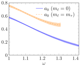
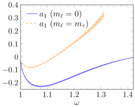
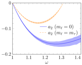
Figure 1: Angular SFs $a_{0},a_{1}$ and $a_{2}$ (Eq. (5)) for the $\Lambda_{b}^{0}\to\Lambda_{c}^{+}\ell^{-}\bar{\nu}_{\ell}$ decay obtained using the LQCD form factors of Ref. Detmold et al. (2015). Bands account for 68% CL intervals deduced from the correlation matrix given in Detmold et al. (2015).

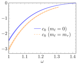
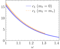
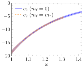
Figure 2: The same as Fig. 1, but for the $c_{0},c_{1}$ and $c_{2}$ SFs defined in the LAB distribution of Eq. (8).

As mentioned above, within the SM, the $c_{2}(\omega)$ SF is the same for all charged leptons, providing a new testing ground for LFU violation studies in $b\to c$ decays. We also observe that finite lepton mass corrections are quite small for $c_{1}$, while become more sizable for the rest of the SFs, which are given here for the very first time using the realistic LQCD results of Ref. Detmold et al. (2015).

For completeness, in Fig. 3 we show the $d\Gamma/d\omega$ differential decay width and its corresponding uncertainty band inherited from the statistical correlated fluctuations of the LQCD form-factors. For the $\tau$ case, we show explicitly the SM predictions for the contributions from tau leptons with positive and negative helicities, both in the CM and LAB frames.

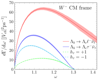
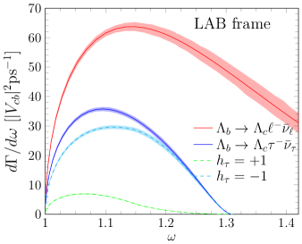
Figure 3: The $d\Gamma/d\omega$ distribution for the $\Lambda_{b}^{0}\to\Lambda_{c}^{+}$ semileptonic decay predicted using the LQCD form factors of Ref. Detmold et al. (2015). The uncertainty bands account for 68% CL intervals, and here $\ell$ stands for a massless charged lepton. For the $\tau$ case we show the individual contributions from tau leptons with positive ($h_{\tau}=1$) and negative ($h_{\tau}=-1$) helicities, measured in the $W^{-}$ CM (left) and in the LAB (right) frames.

III.3 $c_{2}$ and $a_{2}$ sensitivity to NP

In this section we shall investigate the effect of NP on the $c_{2}$ and $a_{2}$ SFs for the $\Lambda_{b}\to\Lambda_{c}$ semileptonic decay. The derived formulas are general and not specific to this transition. We shall consider the effective Hamiltonian

$$H=\frac{4G_{F}|V_{cb}|^{2}}{\sqrt{2}}[(1+C_{V_{L}}){\cal O}_{V_{L}}+C_{V_{R}}{\cal O}_{V_{R}}+C_{S_{L}}{\cal O}_{S_{L}}$$

$$\hskip 71.13188pt+C_{S_{R}}{\cal O}_{S_{R}}+C_{T}{\cal O}_{T}]+h.c.,$$ (17)

taken from Ref. Murgui et al. (2019). The Wilson coefficients, $C_{i}$, parametrize possible deviations from the SM, i.e. $C_{i}^{\rm SM}$=0, and could be in general, lepton and flavour dependent, though in Murgui et al. (2019) are assumed to be present only in the third generation of leptons. Moreover, these LECs are taken to be real (CP-symmetry conserving limit). Complex Wilson coefficients can explain the $b\to c\tau\nu_{\tau}$ anomalies as well as real ones, but they do not offer any clear advantages regarding the fit quality, so they have not been considered in the effective low-energy Hamiltonian approach of Ref. Murgui et al. (2019) for simplicity. In Table 6 of that reference, the authors provide four different fits (4, 5, 6 and 7) that include all the above terms. Of these four fits, we shall only consider the last two. The reason being that for Fits 4 and 5 the SM coefficient is almost canceled and its effect is replaced by NP contributions, what seems to be an unlikely situation from a physical point of view. In Fits 6 and 7 the $C_{T}$ Wilson coefficient is very small ($0.01^{+0.09}_{-0.07}$ and $-0.02^{+0.08}_{-0.07}$, respectively) and here for simplicity we shall make it zero. With these approximations, the amplitude changes from the original current-current $J_{Hrr^{\prime}\,\mu}(p,p^{\prime})\,J_{Lh}^{\mu}(k,k^{\prime})$ term to

$$\widetilde{J}_{Hrr^{\prime}\,\mu}(p,p^{\prime})\,J_{Lh}^{\ \ \mu}(k,k^{\prime})+J_{Hrr^{\prime}}(p,p^{\prime})\,J_{Lh}(k,k^{\prime})\,$$ (18)

where $r,r^{\prime}$ and $h$ are the polarization indexes for the initial and final hadrons and final charged lepton, respectively. Note that $J_{Hrr^{\prime}\,\mu}(p,p^{\prime})$ is the CC current in the general definition of the SM hadron tensor in Eq. (3) (or in Eq. (15) for the $\Lambda_{b}\to\Lambda_{c}$ case) and $J_{Lh}^{\ \ \mu}(k,k^{\prime})=\bar{u}^{(h)}_{\ell}(\vec{k}^{\,\prime}\,)\gamma^{\mu}(1-\gamma_{5})v_{\nu_{\ell}}(\vec{k}\,)$ is the usual vector-axial leptonic current. In turn, $\widetilde{J}_{Hrr^{\prime}\,\mu}(p,p^{\prime})$ is identical to $J_{Hrr^{\prime}\,\mu}(p,p^{\prime})$ but with the vector and axial form factors corrected by the multiplicative factors $C_{V}=(1+C_{V_{L}}+C_{V_{R}})$ and $C_{A}=(1+C_{V_{L}}-C_{V_{R}})$, respectively. As for $J_{Hrr^{\prime}}(p,p^{\prime})$ and $J_{Lt}(k,k^{\prime})$ they are given by

$$J_{Hrr^{\prime}}(p,p^{\prime}) = \langle H_{c};p^{\prime},r^{\prime}|\bar{c}(C_{S}-C_{P}\gamma_{5})b|H_{b};p,r\rangle$$ (19)

$$J_{Lh}(p,p^{\prime}) = \bar{u}^{(h)}_{\ell}(\vec{k}^{\,\prime}\,)(1-\gamma_{5})v_{\nu_{\ell}}(\vec{k}\,).$$ (20)

with $C_{S,P}=(C_{S_{L}}\pm C_{S_{R}})$. The product of the lepton and hadron tensors is now changed to

$$L^{\mu\nu}(k,k^{\prime};h)\,\widetilde{W}_{\mu\nu}(p,q) + L(k,k^{\prime};h)\,W(p,q)$$ (21)

$$+ L_{\mu}(k,k^{\prime};h)\,W^{\mu}(p,q)$$

with $\widetilde{W}_{\mu\nu}(p,q)$ constructed with the vector and axial form factors modified by using the multiplicative factors $C_{V}$ and $C_{A}$ introduced above. In the above expression, $h=\pm 1$ is the charged lepton helicity, with the new lepton terms given by

$$L(k,k^{\prime};h) = \left(k\cdot k^{\prime}+h\,k\cdot s\right)/2$$ (22)

$$L_{\mu}(k,k^{\prime};h) = \frac{m_{\ell}}{2}k_{\mu}+\frac{h}{2m_{\ell}}\left(k^{\prime}_{\mu}k\cdot s-s_{\mu}k\cdot k^{\prime}\right)$$ (23)

while using Lorentz covariance, the hadron new contributions can be expressed as

$$W(p,q) = \overline{\sum}J_{Hrr^{\prime}}(p,p^{\prime})J_{Hrr^{\prime}}^{*}(p,p^{\prime})=W_{SP}$$ (24)

$$W^{\mu}(p,q) = \overline{\sum}\Big{\{}\widetilde{J}^{\mu}_{Hrr^{\prime}}(p,p^{\prime})J_{Hrr^{\prime}}^{*}(p,p^{\prime})$$ (25)

$$+ [\widetilde{J}^{\mu}_{Hrr^{\prime}}(p,p^{\prime})]^{*}J_{Hrr^{\prime}}(p,p^{\prime})\Big{\}}$$

$$= W_{I1}\frac{p^{\mu}}{M}+W_{I2}\frac{q^{\mu}}{M}$$

where we have introduced three new real scalar SFs, $W_{SP},W_{I1}$ and $W_{I2}$, that depend on $q^{2}$ alone. We readily obtain the NP corrections to the double differential decay width $d^{2}\Gamma/(d\omega d\cos\theta_{\ell})$ in the $W^{-}$boson CM frame (Eq. (5)),

$$a_{0} \to \tilde{a}_{0}+\left[\left(W_{SP}+\frac{m_{\ell}}{M}W_{I2}\right)\frac{q^{2}}{M^{2}}+\frac{m_{\ell}M_{\omega}}{M^{2}}W_{I1}\right]$$

$$a_{1} \to \tilde{a}_{1}+\frac{m_{\ell}M^{\prime}}{M^{2}}\sqrt{\omega^{2}-1}W_{I1}$$

$$a_{2} \to \tilde{a}_{2}$$ (26)

where the different $\tilde{a}_{j}$ are given by Eq.(6) with the $W_{1,\cdots,5}$ SFs replaced by their $\widetilde{W}_{1,\cdots,5}$ counterparts that appear in the Lorentz decomposition of $\widetilde{W}_{\mu\nu}(p,q)$. The NP additional corrections to $(\tilde{a}_{i}-a_{i})$ come only from $h=1$, this is to say, they vanish for left helicity charged leptons. Similarly, the NP corrections to the double differential decay width $d^{2}\Gamma/(d\omega dE_{\ell})$ in the LAB frame (Eq. (8)) read

$$c_{0} \to \tilde{c}_{0}+\frac{q^{2}-m_{\ell}^{2}}{M^{2}}\left(W_{SP}+\frac{m_{\ell}}{M}W_{I2}\right)+\frac{2m_{\ell}M_{\omega}}{M^{2}}W_{I1}$$

$$c_{1} \to \tilde{c}_{1}-\frac{2m_{\ell}}{M}W_{I1}$$

$$c_{2} \to \tilde{c}_{2}$$ (27)

where the $\tilde{c}_{j}$ are given by Eq.(8) with the $W_{1,\cdots,5}$ SFs replaced by their corresponding $\widetilde{W}_{1,\cdots,5}$.

Neither $c_{2}$ nor $a_{2}$ are modified by the left and right scalar NP terms, being only sensitive to the left and right vector corrections. Moreover, both of them are now proportional to $\widetilde{W}_{2}$, and hence the relation of Eq. (10) still holds, in this limit where the tensor NP contributions have been neglected.

III.3.1 Results for the $\Lambda_{b}\to\Lambda_{c}$ semileptonic transition

In this case, we have

$$J_{Hrr^{\prime}}(p,p^{\prime})=\bar{u}^{(r^{\prime})}_{\Lambda_{c}}(\vec{p}^{\,\prime}\,)[\,C_{S}F_{S}-C_{P}F_{P}\gamma_{5}\,]u^{(r)}_{\Lambda_{b}}(\vec{p}\,)$$ (28)

where $F_{S}$ and $F_{P}$ are the scalar and pseudoscalar form factors that are directly related (see Eqs. (2.12) and (2.13) of Ref. Datta et al. (2017)) to the $f_{0}$ vector and $g_{0}$ axial ones given in Detmold et al. (2015) . We thus have

$$W_{SP} = \frac{1}{2}{\rm Tr}\Bigg{[}\frac{\not{p}^{\prime}+M_{\Lambda_{c}}}{2M_{\Lambda_{c}}}\left(C_{S}F_{S}-C_{P}F_{P}\gamma_{5}\right)$$ (29)

$$\times \frac{\not{p}+M_{\Lambda_{b}}}{2M_{\Lambda_{b}}}\left(C_{S}F_{S}+C_{P}F_{P}\gamma_{5}\right)\Bigg{]}$$

while the interference hadron tensor reads

$$W_{\mu}(p,q)=\frac{1}{2}{\rm Tr}\Bigg{[}\frac{\not{p}^{\prime}+M_{\Lambda_{c}}}{2M_{\Lambda_{c}}}\widetilde{\cal O}_{\mu}\frac{\not{p}+M_{\Lambda_{b}}}{2M_{\Lambda_{b}}}\left(C_{S}F_{S}+C_{P}F_{P}\gamma_{5}\right)+\frac{\not{p}^{\prime}+M_{\Lambda_{c}}}{2M_{\Lambda_{c}}}\left(C_{S}F_{S}-C_{P}F_{P}\gamma_{5}\right)\frac{\not{p}+M_{\Lambda_{b}}}{2M_{\Lambda_{b}}}\gamma^{0}\widetilde{\cal O}_{\mu}^{\dagger}\gamma^{0}\Bigg{]}$$ (30)

with $\widetilde{\cal O}^{\mu}=\Bigg{(}\sum_{i=1}^{3}{\cal O}^{\mu}_{i}\widetilde{\cal F}_{i}\Bigg{)}$ and $\widetilde{\cal F}_{i}=(C_{V}\,F_{i}-\gamma_{5}C_{A}G_{i}),\,i=1,2,3$. Expressions for $W_{SP},W_{I1}$ and $W_{I2}$ in terms of $\widetilde{F}_{S,P}=C_{S,P}F_{S,P}$ (Eq. (28)), $\widetilde{F}_{i}=C_{V}F_{i}$ and $\widetilde{G}_{i}=C_{A}G_{i}$ are given in Appendix B.

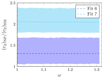
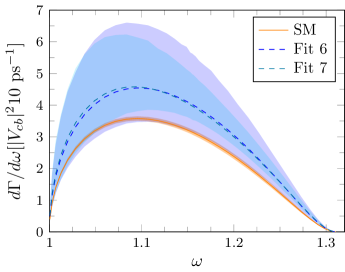
Figure 4: Left: $(c_{2})_{NP}/(c_{2})_{SM}$ ratio for the $\Lambda_{b}\to\Lambda_{c}$ semileptonic transition obtained with the parameters of Fits 6 and 7 in Ref. Murgui et al. (2019). Right: SM and NP predictions for the $d\Gamma/d\omega$ distribution for the $\tau$ decay mode. As in other figures, the LQCD form factors of Ref. Detmold et al. (2015) have been used and the uncertainty bands account for 68% CL intervals.

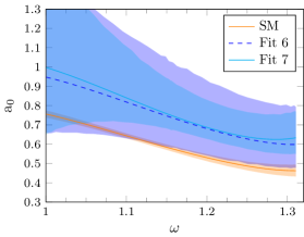
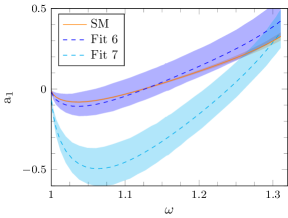
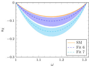
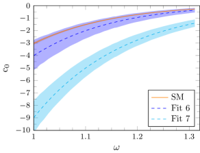
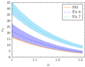
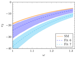
Figure 5: CM angular $a_{0},a_{1}$ and $a_{2}$ (top) and LAB $\tau-$energy $c_{0},c_{1}$ and $c_{2}$ (bottom) SFs for the $\Lambda_{b}^{0}\to\Lambda_{c}^{+}\tau^{-}\bar{\nu}_{\tau}$ decay obtained using the LQCD form factors of Ref. Detmold et al. (2015). As in Fig. 4, we show the SM predictions and the NP results obtained from Fits 6 and 7 of Ref. Murgui et al. (2019).

As mentioned above, $c_{2}$ and $a_{2}$ are not affected by the left and right scalar NP terms and these SFs are only modified by the left and right vector Wilson coefficients $C_{V_{L},V_{R}}$. This turns out to be very relevant. Fits 6 and 7 in Ref. Murgui et al. (2019) provide very different values for $C_{V_{L}}$ and $C_{V_{R}}$ which implies different NP changes in $c_{2}$ and $a_{2}$ SFs. However, the two fits produce very similar results for the ${\cal R}_{\Lambda_{c}}$ ratio (roughly 0.42, to be compared to the SM prediction of $0.33\pm 0.02$). In this situation the $c_{2}$ or $a_{2}$ SFs are observables that could differentiate one fit from the other. In the left panel of Fig. 4 we show the ratio $(c_{2})_{NP}/(c_{2})_{SM}=(a_{2})_{NP}/(a_{2})_{SM}$ as a function of $\omega$ for the two fits under consideration. The $\omega$ dependence is hardly visible (for an explanation see the discussion below) but, as seen in the figure, the changes in magnitude of the NP corrections are significantly different in the two fits, and are not accounted for by errors. Hence, a measurement of $c_{2}$ for $\tau$ decay would not only be a direct measurement of the possible existence of NP, but it would also allow to distinguish from fits that otherwise give the same total and differential $d\Gamma/d\omega$ decay widths (see right panel of Fig. 4). It would thus provide information on the type of NP that is needed to explain the data.

For completeness in Fig. 5, we show the CM angular $a_{0},a_{1}$ and $a_{2}$ (top) and LAB $\tau-$energy $c_{0},c_{1}$ and $c_{2}$ (bottom) SFs as functions of $\omega$. In addition to $c_{2}$ and $a_{2}$, we find that $a_{1}$, and both $c_{0}$ and $c_{1}$ can also be used to distinguish between the two NP scenarios related to the minima 6 and 7 of Ref. Murgui et al. (2019). We recall here that the NP parameters were obtained in that reference from a general model-independent analysis of $b\to c\tau\bar{\nu}_{\tau}$ transitions, including measurements of ${\cal R}_{D}$, ${\cal R}_{D^{*}}$, their $q^{2}$ differential distributions, the recently measured longitudinal $D^{*}$ polarization $F_{L}^{D^{*}}$, and constraints from the $B_{c}\to\tau\bar{\nu}_{\tau}$ lifetime. We would like to stress that all $c_{0},c_{1}$ and $c_{2}$ SFs, that determine the LAB $d^{2}\Gamma/(d\omega dE_{\ell})$ distribution, are quite differently affected by the two NP settings analyzed here, even though both give rise to indistinguishable $d^{2}\Gamma/d\omega$ differential decay widths.

Moreover, we also see that the ratio $(a_{1})_{NP}/(a_{1})_{SM}$ would exhibit some sizable $\omega-$dependence, in particular in the case of Fit 7. This is in contrast to the case of the $(c_{2})_{NP}/(c_{2})_{SM}$ ratio, depicted in the left panel of Fig. 4, that turned out to be practically flat. This is because only linear $C_{V_{R}}$ terms could induce a non-zero $\omega$ dependence for $(c_{2})_{NP}/(c_{2})_{SM}$, but however, to a high degree of aproximation (it would be exact in the heavy quark limit), $\widetilde{W}_{2}$ is given by $M_{\Lambda_{b}}(\widetilde{F}_{1}^{2}(\omega)+\widetilde{G}_{1}^{2}(\omega))/M_{\Lambda_{c}}$ with $F_{1}(\omega)\sim G_{1}(\omega)$ and, in this approximation linear effects on $C_{V_{R}}$ cancel exactly.

In the discussions on Figs. 4 and 5 above, we have assumed uncorrelated Gaussian distributions for the Wilson coefficients $C_{V_{L}}$, $C_{V_{R}}$, $C_{S_{L}}$ and $C_{S_{R}}$ and have averaged the asymmetric errors quoted in Ref. Murgui et al. (2019), since correlation matrices are not provided in that reference. This should be sufficient for the illustrative purposes of this subsection. Nevertheless, in what follows we will estimate the effects produced by the correlations between the Wilson coefficients in the $(c_{2})_{NP}/(c_{2})_{SM}$ ratio.

Note that in Ref. Murgui et al. (2019), the uncertainties of a given parameter $y_{i}$ was determined as the shifts $\Delta y_{i}$ around the best-fit value $y^{\rm min}_{i}$ of that parameter, such that the minimization of $\chi^{2}|_{y_{i}=y^{\rm min}_{i}+\Delta y_{i}}$ varying all remaining parameters in the vicinity of the minimum leads to an increase $\Delta\chi^{2}=1$. This procedure leads, in general, to asymmetric errors, and to non-Gaussian correlations that cannot be accounted for by a single matrix. The effects of these correlations on $(c_{2})_{NP}/(c_{2})_{SM}$ are shown in Fig. 6. We have chosen this ratio because it hardly depends on $\omega$, and thus in Fig. 6 we have fixed it to the intermediate value of 1.15. In the left (Fit 6) and middle (Fit 7) panels of this figure, we depict $(c_{2})_{NP}/(c_{2})_{SM}|_{\omega=1.15}$ and ${\cal R}_{\Lambda_{c}}$ for several sets of Wilson coefficients, which give rise to the ${\cal R}_{D}$ and ${\cal R}_{D^{*}}$ values given in the bottom and top $X-$axes.

The ratios ${\cal R}_{D}$, ${\cal R}_{D^{*}}$ and ${\cal R}_{\Lambda_{c}}$ (black dashed-curves in the bottom plots), and the $\chi^{2}$ shown in the right panel of Fig. 6 have been computed as described in  Murgui et al. (2019) and have been obtained from the authors of that reference Peñuelas and Murgui . In Fig. 6, the Wilson-coefficients space is scanned starting from Fit 6 and 7 minima, through successive small steps in the multi-parameter space leading to moderate merit-function enhancements and ${\cal R}_{\Lambda_{c}}$ variations (see the right plot of Fig. 6). There exist one-to-one relations between each set of Wilson coefficients (sWC) used in the left (Fit 6) and middle (Fit 7) panels of Fig. 6 and the chi-square values or the variations $\Delta{\cal R}_{\Lambda_{c}}(={\cal R}_{\Lambda_{c}}^{\rm sWC}-{\cal R}_{\Lambda_{c}}^{\min})$ shown in the right plot of the figure. Note that at some point for $\Delta{\cal R}_{\Lambda_{c}}<-0.02$, the local Fit 7 collapses into Fit 6.

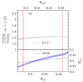
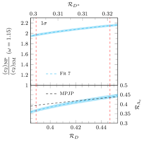
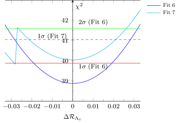
Figure 6: Left and middle panels: Effects of Wilson-coefficients statistical correlations on $(c_{2})_{NP}/(c_{2})_{SM}|_{\omega=1.15}$ for the NP Fits 6 and 7 of Ref. Murgui et al. (2019). Each set of Wilson coefficients is identified by its predictions for ${\cal R}_{D}$ and ${\cal R}_{D^{*}}$ ($X-$axes) and ${\cal R}_{\Lambda_{c}}$ (black dashed-curve, labelled as MPJP, in the bottom plots) Murgui et al. (2019); Peñuelas and Murgui . SM predictions for the ${\cal R}_{D}^{\rm SM}=0.300\pm 0.05$ and ${\cal R}_{D^{*}}^{\rm SM}=0.251\pm 0.004$ ratios are below the ranges considered, while ${\cal R}^{\rm SM}_{\Lambda_{c}}=0.33\pm 0.02$. We also show ${\cal R}_{\Lambda_{c}}$ computed after neglecting the NP tensor contribution (magenta and cyan dashed-lines for Fits 6 and 7, respectively). Shaded bands in our baryon results stand for 68% CL uncertainties inherited from LQCD inputs Detmold et al. (2015). Right panel: Fits 6 and 7 chi-square values Murgui et al. (2019); Peñuelas and Murgui for each set of Wilson coefficients (sWC) used in the left and middle panels, and represented in this plot by $\Delta{\cal R}_{\Lambda_{c}}={\cal R}_{\Lambda_{c}}^{\rm sWC}-{\cal R}_{\Lambda_{c}}^{\min}$, with ${\cal R}_{\Lambda_{c}}^{\min}=0.405$ and 0.415 for Fits 6 and 7, respectively. See text for more details.

We see that Fit 6 and 7 chi-squares grow from their local minimum values, and the $\Delta\chi^{2}=1$ and $\Delta\chi^{2}=2.71$ increments can be used Murgui et al. (2019) to determine the 68% ($1\sigma$) and 90% ($2\sigma$) CL intervals of the NP predictions for ${\cal R}_{D}$, ${\cal R}_{D^{*}}$ and ${\cal R}_{\Lambda_{c}}$. We also use here these $\chi^{2}$ variations to estimate the uncertainties on the results for $(c_{2})_{NP}/(c_{2})_{SM}|_{\omega=1.15}$. In addition, the 68% CL errors induced from the $\Lambda_{b}\to\Lambda_{c}$ LQCD form-factors Detmold et al. (2015) are very small for this ratio, and are showed by the shaded bands in both plots. Comparing the results depicted in Fig. 4 with the variation of $(c_{2})_{NP}/(c_{2})_{SM}|_{\omega=1.15}\left[=(a_{2})_{NP}/(a_{2})_{SM}|_{\omega=1.15}\right]$ between the $1\sigma$-vertical lines shown in Fig. 6, we observe that the inclusion of the Wilson-coefficients statistical correlations reduces the uncertainties on this ratio by factors of five and three for the predictions obtained from Fits 6 and 7, respectively. Thus, now we find that these two NP scenarios give rise to results for this latter observable separated by more than 5$\sigma$, $1.40\pm 0.04$ versus $2.06\pm 0.09$, despite predicting fully compatible ${\cal R}_{D}$, ${\cal R}_{D^{*}}$ and ${\cal R}_{\Lambda_{c}}$ integrated ratios. This discussion strongly reinforces our previous conclusions from Fig. 4.

A final remark concerns on the errors induced by neglecting the tensor NP contribution. In the bottom plots of the first two panels of Fig. 6, we compare for different sets of Wilson coefficients, the predictions for ${\cal R}_{\Lambda_{c}}$ obtained from the full model of Ref. Murgui et al. (2019) (MPJP black dashed-curves) with those obtained in this work (magenta and cyan dashed-lines), where $C_{T}$ has been set to zero. For the latter predictions, we also display the errors (68% CL bands) inherited from the $\Lambda_{b}\to\Lambda_{c}$ LQCD form-factors. We see that within the $1\sigma$ intervals, both for Fit 6 and 7, the effects of the NP tensor term on ${\cal R}_{\Lambda_{c}}$ are moderately small, and are partially accounted for the uncertainties of the LQCD inputs. This continues to be the case for all sets of Fit 7 Wilson coefficients considered in the $\chi^{2}-$plot of Fig. 6, while for Fit 6 and in regions above 1$\sigma$, $|C_{T}|$ appreciably grows and its effects become sizable.

IV Summary

We have introduced a general framework, valid for any $H\to H^{\prime}\ell\nu_{\ell}$ semileptonic decay, to study the lepton polarized CM $d^{2}\Gamma/(d\omega d\cos\theta_{\ell})$ and LAB $d^{2}\Gamma/(d\omega dE_{\ell})$ differential decay widths. To our knowledge, this is the first time that the relevance of the $d^{2}\Gamma/(d\omega dE_{\ell})$ differential decay width has been put forward as a candidate for LFU violation studies in $b\to c$ decays. Specifically, within the SM the $c_{2}(\omega)$ SF appearing in that distribution is the same for all charged leptons. That makes it a perfect quantity for LFU violation studies. We have also found a correlation between the $a_{2}(\omega)$ SF related to the $(\cos\theta_{\ell})^{2}$ dependence in $d^{2}\Gamma/(d\omega d\cos\theta_{\ell})$ and $c_{2}(\omega)$. This correlation is shown in Eq. (10) and states that the ratio $a_{2}(\omega)/c_{2}(\omega)$, corrected by trivial kinematical and mass factors, gives a universal function valid for any $H\to H^{\prime}$ semileptonic decay. Again, this is a clear prediction of the SM that can be checked against experiment. These two results could play a relevant role as further tests of the SM and LFU.

We have also generalized the formalism to account for some NP terms, and shown that neither $c_{2}$ nor $a_{2}$ are modified by left and right scalar NP terms, being however sensitive to left and right vector corrections. We also found that the relation of Eq. (10) for the $a_{2}/c_{2}$ ratio is not modified by these latter NP contributions.

Finally, we have presented SM and NP predictions for the $\Lambda_{b}\to\Lambda_{c}$ transition. We have shown that a measurement of $c_{2}$ (or $a_{2}$) for $\tau$ decay would not only be a direct measurement of the possible existence of NP, but it would also allow to distinguish from NP fits to $b\to c\tau\bar{\nu}_{\tau}$ anomalies in the meson sector, that otherwise give the same total and differential $d\Gamma/d\omega$ widths. The same applies to the other two SFs, $c_{0}$ and $c_{1}$, that appear in the LAB $d^{2}\Gamma/(d\omega dE_{\ell})$ differential width, and for the $a_{1}$ coefficient ($\cos\theta_{\ell}$ linear term) in the CM angular distribution.

Appendix A Hadron tensor SFs and form-factors for the $\Lambda_{b}^{0}\to\Lambda_{c}^{+}\ell^{-}\bar{\nu}_{\ell}$ decay

The form factors used in Eq. (15) are related to those used in Ref. Detmold et al. (2015) by

$$F_{1} = f_{\perp},$$

$$F_{2} = \frac{M_{\Lambda_{b}}\delta_{M_{\Lambda}}}{q^{2}}f_{0}+\frac{M_{\Lambda_{b}}\Delta_{M_{\Lambda}}}{s_{+}}\left[1-\delta\right]f_{+}-\delta_{s_{+}}f_{\perp},$$

$$F_{3} = -\frac{M_{\Lambda_{c}}\delta_{M_{\Lambda}}}{q^{2}}f_{0}+\frac{M_{\Lambda_{c}}\Delta_{M_{\Lambda}}}{s_{+}}\left[1+\delta\right]f_{+}-\delta_{s_{+}}f_{\perp},$$

$$G_{1} = g_{\perp},$$

$$G_{2} = -\frac{M_{\Lambda_{b}}\Delta_{M_{\Lambda}}}{q^{2}}g_{0}-\frac{M_{\Lambda_{b}}\delta_{M_{\Lambda}}}{s_{-}}\left[1-\delta\right]g_{+}-\delta_{s_{-}}g_{\perp},$$

$$G_{3} = \frac{M_{\Lambda_{c}}\Delta_{M_{\Lambda}}}{q^{2}}g_{0}-\frac{M_{\Lambda_{c}}\delta_{M_{\Lambda}}}{s_{-}}\left[1+\delta\right]g_{+}+\delta_{s_{-}}g_{\perp},$$

with $\delta=(M_{\Lambda_{b}}^{2}-M_{\Lambda_{c}}^{2})/q^{2}$, $s_{\pm}=(M_{\Lambda_{b}}\pm M_{\Lambda_{c}})^{2}-q^{2}$, $\delta_{M_{\Lambda}}=M_{\Lambda_{b}}-M_{\Lambda_{c}}$, $\Delta_{M_{\Lambda}}=M_{\Lambda_{b}}+M_{\Lambda_{c}}$ and $\delta_{s_{\pm}}=2M_{\Lambda_{b}}M_{\Lambda_{c}}/s_{\pm}$.

On the other hand, from Eqs. (16) and (4), we find

$$W_{1} = \frac{1}{2}\Big{[}(\omega-1)F_{1}^{2}+(\omega+1)G_{1}^{2}\Big{]},$$

$$W_{2} = \frac{1}{2}\left\{2F_{1}F_{2}+(\omega+1)F_{2}^{2}+2G_{1}G_{2}+(\omega-1)G_{2}^{2}+\frac{2M_{\Lambda_{b}}}{M_{\Lambda_{c}}}\Big{[}(F_{1}+F_{2})(F_{1}+F_{3})+\omega(F_{2}F_{3}+G_{2}G_{3})\right.$$

$$+ \left.(G_{1}-G_{2})(G_{1}+G_{3})\Big{]}+\frac{M_{\Lambda_{b}}^{2}}{M_{\Lambda_{c}}^{2}}\Big{[}2F_{1}F_{3}+(\omega+1)F_{3}^{2}+(\omega-1)G_{3}^{2}-2G_{1}G_{3}\Big{]}\right\},$$

$$W_{3} = \frac{2M_{\Lambda_{b}}}{M_{\Lambda_{c}}}F_{1}G_{1},$$

$$W_{4} = \frac{M_{\Lambda_{b}}^{2}}{2M_{\Lambda_{c}}^{2}}\Big{[}2F_{1}F_{3}+(\omega+1)F_{3}^{2}+(\omega-1)G_{3}^{2}-2G_{1}G_{3}\Big{]},$$

$$W_{5} = -\frac{M_{\Lambda_{b}}}{M_{\Lambda_{c}}}\Big{[}(F_{1}+F_{2})(F_{1}+F_{3})+\omega(F_{2}F_{3}+G_{2}G_{3})+(G_{1}-G_{2})(G_{1}+G_{3})\Big{]}$$

$$- \frac{M_{\Lambda_{b}}^{2}}{M_{\Lambda_{c}}^{2}}\Big{[}2F_{1}F_{3}+(\omega+1)F_{3}^{2}+(\omega-1)G_{3}^{2}-2G_{1}G_{3}\Big{]}.$$

Appendix B NP effects on the hadron SFs for the $\Lambda_{b}^{0}\to\Lambda_{c}^{+}\ell^{-}\bar{\nu}_{\ell}$ decay

From Eqs. (29) and (30), we find

$$W_{SP} = \frac{1}{2}\Big{[}(\omega+1)\widetilde{F}_{S}^{2}+(\omega-1)\widetilde{F}_{P}^{2}\Big{]},$$

$$W_{I1} = -W_{I2}+\widetilde{F}_{S}\left(\widetilde{F}_{1}+(1+\omega)\widetilde{F}_{2}\right)+\widetilde{F}_{P}\left(\widetilde{G}_{1}-(1-\omega)\widetilde{G}_{2}\right),$$

$$W_{I2} = \frac{M_{\Lambda_{b}}}{M_{\Lambda_{c}}}\left[\widetilde{F}_{P}\left(\widetilde{G}_{1}+(1-\omega)\widetilde{G}_{3}\right)-\widetilde{F}_{S}\left(\widetilde{F}_{1}+(1+\omega)\widetilde{F}_{3}\right)\right]$$ (33)

and $F_{S}=(M_{\Lambda_{b}}-M_{\Lambda_{c}})f_{0}/(m_{b}-m_{c})$, $F_{P}=(M_{\Lambda_{b}}+M_{\Lambda_{c}})g_{0}/(m_{b}+m_{c})$. In the numerical calculations, we use $m_{b}=4.18\pm 0.04$ GeV and $m_{c}=1.27\pm 0.03$ GeV as in Ref. Datta et al. (2017).

References

- Bifani et al. (2019) S. Bifani, S. Descotes-Genon, A. Romero Vidal, and M.-H. Schune, J. Phys. G46, 023001 (2019), arXiv:1809.06229 [hep-ex] .
- Amhis et al. (2017) Y. Amhis et al. (HFLAV), Eur. Phys. J. C77, 895 (2017), online update at https://hflav.web.cern.ch/, arXiv:1612.07233 [hep-ex] .
- Lees et al. (2012) J. P. Lees et al. (BaBar), Phys. Rev. Lett. 109, 101802 (2012), arXiv:1205.5442 [hep-ex] .
- Lees et al. (2013) J. P. Lees et al. (BaBar), Phys. Rev. D88, 072012 (2013), arXiv:1303.0571 [hep-ex] .
- Huschle et al. (2015) M. Huschle et al. (Belle), Phys. Rev. D92, 072014 (2015), arXiv:1507.03233 [hep-ex] .
- Sato et al. (2016) Y. Sato et al. (Belle), Phys. Rev. D94, 072007 (2016), arXiv:1607.07923 [hep-ex] .
- Hirose et al. (2017) S. Hirose et al. (Belle), Phys. Rev. Lett. 118, 211801 (2017), arXiv:1612.00529 [hep-ex] .
- Aaij et al. (2015) R. Aaij et al. (LHCb), Phys. Rev. Lett. 115, 111803 (2015), [Erratum: Phys. Rev. Lett.115,no.15,159901(2015)], arXiv:1506.08614 [hep-ex] .
- Aaij et al. (2018) R. Aaij et al. (LHCb), Phys. Rev. Lett. 120, 171802 (2018), arXiv:1708.08856 [hep-ex] .
- Aoki et al. (2017) S. Aoki et al., Eur. Phys. J. C77, 112 (2017), arXiv:1607.00299 [hep-lat] .
- Bigi and Gambino (2016) D. Bigi and P. Gambino, Phys. Rev. D94, 094008 (2016), arXiv:1606.08030 [hep-ph] .
- Jaiswal et al. (2017) S. Jaiswal, S. Nandi, and S. K. Patra, JHEP 12, 060 (2017), arXiv:1707.09977 [hep-ph] .
- Abdesselam et al. (2019) A. Abdesselam et al. (Belle), (2019), arXiv:1904.08794 [hep-ex] .
- Murgui et al. (2019) C. Murgui, A. Peñuelas, M. Jung, and A. Pich, JHEP 09, 103 (2019), arXiv:1904.09311 [hep-ph] .
- Fajfer et al. (2012) S. Fajfer, J. F. Kamenik, and I. Nisandzic, Phys. Rev. D85, 094025 (2012), arXiv:1203.2654 [hep-ph] .
- Aaij et al. (2017) R. Aaij et al. (LHCb), Phys. Rev. D96, 112005 (2017), arXiv:1709.01920 [hep-ex] .
- Cerri et al. (2018) A. Cerri et al., (2018), arXiv:1812.07638 [hep-ph] .
- Neubert (1994) M. Neubert, Phys. Rept. 245, 259 (1994), arXiv:hep-ph/9306320 [hep-ph] .
- Bernlochner et al. (2018) F. U. Bernlochner, Z. Ligeti, D. J. Robinson, and W. L. Sutcliffe, Phys. Rev. Lett. 121, 202001 (2018), arXiv:1808.09464 [hep-ph] .
- Detmold et al. (2015) W. Detmold, C. Lehner, and S. Meinel, Phys. Rev. D92, 034503 (2015), arXiv:1503.01421 [hep-lat] .
- Blanke et al. (2019a) M. Blanke, A. Crivellin, S. de Boer, M. Moscati, U. Nierste, I. Nišandžić, and T. Kitahara, Phys. Rev. D99, 075006 (2019a).
- Blanke et al. (2019b) M. Blanke, A. Crivellin, T. Kitahara, M. Moscati, U. Nierste, and I. Nišandžić, Phys. Rev. D 100, 035035 (2019b).
- Böer et al. (2019) P. Böer, A. Kokulu, J.-N. Toelstede, and D. van Dyk, (2019), arXiv:1907.12554 [hep-ph] .
- Shivashankara et al. (2015) S. Shivashankara, W. Wu, and A. Datta, Phys. Rev. D 91, 115003 (2015).
- Li et al. (2017) X.-Q. Li, Y.-D. Yang, and X. Zhang, JHEP 02, 068 (2017), arXiv:1611.01635 [hep-ph] .
- Datta et al. (2017) A. Datta, S. Kamali, S. Meinel, and A. Rashed, JHEP 08, 131 (2017), arXiv:1702.02243 [hep-ph] .
- Bernlochner et al. (2019) F. U. Bernlochner, Z. Ligeti, D. J. Robinson, and W. L. Sutcliffe, Phys. Rev. D99, 055008 (2019), arXiv:1812.07593 [hep-ph] .
- Ray et al. (2019) A. Ray, S. Sahoo, and R. Mohanta, Phys. Rev. D99, 015015 (2019), arXiv:1812.08314 [hep-ph] .
- Di Salvo et al. (2018) E. Di Salvo, F. Fontanelli, and Z. J. Ajaltouni, Int. J. Mod. Phys. A33, 1850169 (2018), arXiv:1804.05592 [hep-ph] .
- Ferrillo et al. (2019) M. Ferrillo, A. Mathad, P. Owen, and N. Serra, (2019), arXiv:1909.04608 [hep-ph] .
- Tanabashi et al. (2018) M. Tanabashi et al. (Particle Data Group), Phys. Rev. D98, 030001 (2018), and 2019 update.
- Hernandez et al. (2007) E. Hernandez, J. Nieves, and M. Valverde, Phys. Rev. D76, 033005 (2007), arXiv:hep-ph/0701149 [hep-ph] .
- Sobczyk et al. (2018) J. E. Sobczyk, E. Hernández, S. X. Nakamura, J. Nieves, and T. Sato, Phys. Rev. D98, 073001 (2018), arXiv:1807.11281 [hep-ph] .
- Bourrely et al. (2009) C. Bourrely, I. Caprini, and L. Lellouch, Phys. Rev. D79, 013008 (2009), [Erratum: Phys. Rev.D82,099902(2010)], arXiv:0807.2722 [hep-ph] .
- Azizi and Süngü (2018) K. Azizi and J. Y. Süngü, Phys. Rev. D97, 074007 (2018).
- (36) A. Peñuelas and C. Murgui, private communication .