Dynamic Processes of the Moreton Wave on 2014 March 29

Abstract

On 2014 March 29, an intense solar flare classified as X1.0 occurred in the active region 12017. Several associated phenomena accompanied this event, among them a fast-filament eruption, large-scale propagating disturbances in the corona and the chromosphere including a Moreton wave, and a coronal mass ejection. This flare was successfully detected in multiwavelength imaging in H$\alpha$ line by the Flare Monitoring Telescope (FMT) at Ica University, Peru. We present a detailed study of the Moreton wave associated with the flare in question. Special attention is paid to the Doppler characteristics inferred from the FMT wing (H$\alpha$ $\pm 0.8$ Å) observations, which are used to examine the downward/upward motion of the plasma in the chromosphere. Our findings reveal that the downward motion of the chromospheric material at the front of the Moreton wave attains a maximum velocity of $4~{}\rm{km~{}s^{-1}}$, whereas the propagation speed ranges between $640$ and $859~{}{\rm~{}km~{}s^{-1}}$. Furthermore, utilizing the weak shock approximation in conjunction with the velocity amplitude of the chromospheric motion induced by the Moreton wave, we derive the Mach number of the incident shock in the corona. We also performed the temperature-emission measure analysis of the coronal wave based on the Atmospheric Imaging Assembly (AIA) observations, which allowed us to derive the compression ratio, and to estimate the Alfvén and fast-mode Mach numbers of the order of 1.06–1.28 and 1.05–1.27. Considering these results and the MHD linear theory we discuss the characteristics of the shock front and the interaction with the chromospheric plasma.

1 Introduction

Shock waves associated with explosive events are fundamental physical processes in the solar atmosphere, whose properties and effects have widely been discussed in the framework of magnetohydrodynamics (MHD) theory. In the Sun’s chromosphere a large-scale wavelike propagating disturbance, that was discovered by Moreton (1960) and Moreton & Ramsey (1960) during the observation of a solar flare in the wing of the H$\alpha$ line, occasionally happens in association with strong flares. This wave phenomenon known as “Moreton wave” usually propagates as semicircular fronts through the chromosphere over a distance of about $5\times 10^{5}~{}\rm{km}$ from the flaring region, at the speed of the order of $500-1500~{}\rm{km~{}s}^{-1}$. Associated with Moreton waves, filaments and prominences standing in the way of propagation direction can abruptly be induced to oscillate, and in some situations to a disruption. Observations in H$\alpha$ spectral line reveal that the leading front of the Moreton wave is observed as enhanced absorption in the red-wing and as reduced absorption (brightening) in the blue-wing, followed by a fainter reversed front, as enhanced absorption in the blue-wing and as reduced absorption in the red-wing (Dodson & Hedeman, 1968). In the core of H$\alpha$ line the wave fronts usually appear as brightening. These observational characteristics were interpreted as depression and a subsequent relaxation process of the chromospheric material, as a consequence of the plasma being forced to move downward with a velocity of $6-10~{}\rm{km~{}s}^{-1}$ (Švestka, 1976) inferred from the motions of spicules and fibrils caused by the wave front passage.

The kinematical properties of the Moreton wave such as the high speed, the great traveling distances, and the low wave amplitude, led to the question whether or not this phenomenon is of chromospheric origin; since the mentioned physical parameters are incompatible with the framework of wave propagation in the chromosphere. For example, for a typical value of the temperature in the chromosphere of $10^{4}~{}\rm{K}$, the sound speed results in $\sim$$10~{}\rm{km~{}s^{-1}}$, and assuming a density $10^{11}~{}\rm{cm^{-3}}$ and $15~{}\rm{G}$ of magnetic field, the Alfvén speed in the chromosphere is about $100~{}\rm{km~{}s^{-1}}$. A wave traveling in the chromosphere with a speed of $1000~{}\rm{km~{}s^{-1}}$, as determined from observations, would imply that this wave moves with a Mach number of the order of 10. A shock wave of such strength should exhibit a strong amplitude and would fully be dissipated before traveling long distances, however, those effects are not observed. A comprehensive interpretation on the generation and propagation aspects of the Moreton wave is conducted if wave propagation in the corona is considered, where the sound and Alfvén speeds are about one order of magnitude larger than in the chromosphere. This idea was initially postulated by Anderson (1966) and Meyer (1968), and further modeled by Uchida (1968). According to Uchida’s model, the pressure pulse during the explosive phase of a solar flare generates an MHD fast-mode wave in the corona, which compresses and pushes downward the chromospheric plasma, and as a result the Moreton wave is created. A good correlation between type II radio burst and Moreton waves does exit (Kai, 1970). Since the former traces the upward propagating fast-mode shock in the corona, it supports the Uchida’s scenario.

In 1997, a large-scale wave propagating disturbance was discovered in coronal emission line Fe xii (195 Å) in association with an C-class flare (Thompson et al., 1999). This coronal wave, named as “EIT wave” after the Extreme-ultraviolet Imaging Telescope (EIT; Delaboudinière et al., 1995) on board the Solar and Heliospheric Observatory (SOHO; Domingo et al., 1995), was expected to be the fast-mode MHD counterpart of the Moreton wave as predicted by Uchida (1968). However, over the last 20 years there was an intense debate in interpreting this phenomenon as an MHD fast-mode wave (see reviews by Chen, 2016; Long et al., 2017). The controversy resides in its physical nature, such as the long-lasting coronal dimming, stationary brightening, and particularly its traveling speed; since it ranges between $170-350~{}\rm{km~{}s^{-1}}$ Klassen et al. (2000); Thompson & Myers (2009) being slower than the expected fast-mode speed, and sometimes even slower than the sound speed in the corona (Thompson & Myers, 2009). In addition, the EIT waves lack the correlation with type II radio bursts, whose speed is in the range of $300-1200~{}\rm{km~{}s^{-1}}$ (Klassen et al., 2000). In order to overcome the discrepancies on the nature of the EIT and Moreton waves, several models and possibilities were put forward. For example, based on MHD simulations by Chen et al. (2002) and extending them, Chen, Fang, & Shibata (2005) found that an upward-expanding flux-rope is capable to trigger a coronal mass ejection (CME) by which two wavelike propagating disturbances are produced: a fast-mode shock wave, and a slower component related to the density perturbation resulting from successive stretching field lines that overlies the erupting flux-rope. Here it is worth noticing that Delannée & Aulanier (1999) identified a bright front in EIT images associated with a flare and CME, and they proposed a scenario of magnetic field reconfiguration as a model of EIT waves. Alternative interpretations have also been suggested in order to clarify the inconsistency of the velocity between the EIT and Moreton waves, such as a subsequent deceleration (Warmuth et al., 2001), which was explained in terms of fast-mode shock produced by a “blast wave” rather than a flux-rope expansion. Note that in the meantime, large-scale disturbances associated with flares traveling through the corona were also detected in soft X-ray emission (e.g., Khan & Aurass, 2002; Narukage et al., 2002; Hudson et al., 2003; Warmuth et al., 2005; Asai et al., 2008), and reported in radio wavelengths as type II burst (e.g., Khan & Aurass, 2002; Eto et al., 2002; Vršnak et al., 2005). They were interpreted as the coronal counterpart of Moreton waves.

Nearly a decade, the Atmospheric Imaging Assembly (AIA; Lemen et al., 2012) instrument on board the Solar Dynamics Observatory (SDO; Pesnell et al., 2012) is constraining our understanding of coronal waves. From now on, in this paper we will use the term “EUV waves” for referring large-scale coronal disturbances observed in extreme ultraviolet (EUV) passbands. Thanks to the AIA’s unprecedented capability, significant discoveries were possible, including intrinsic characteristics never seen before of the coronal EUV waves. So, it is more likely that the controversy on the EIT waves is coming to an end. Nowadays, it is being more accepted that two kinds of large-scale wavelike phenomena appear in the corona in association with flares and CMEs. The first, the MHD fast-mode or shock traveling ahead, and the second or slow component straddling behind. This picture was initially reported by Harra & Sterling (2003) based on TRACE (Handy et al., 1999) observations, suggested by analytical and numerical approaches (e.g., Chen et al., 2002), and is being confirmed by numerous recent studies (cf. Liu & Ofman, 2014; Warmuth, 2015). It was also found a clear evidence of co-spatiality between the fast-mode EUV wave and the Moreton wave (Asai et al., 2012), and the association with type II radio burst displays a high tendency (Nitta et al., 2013). It should be mentioned that statistical investigations have shown that EUV waves are more linked to CMEs rather than solar flares (Biesecker et al., 2002; Nitta et al., 2013, 2014; Muhr et al., 2014), although the mechanism by which they are related still remains puzzling.

The 2014 March 29 flare is one of the best observed event, because it was captured in a wide range of wavelengths with unprecedented temporal and spatial resolution by advanced space-borne and ground-based instruments. This powerful flare classified as X1.0 on the GOES scale occurred in the active region 12017 (N11, W32), and was accompanied by various associated phenomena: a fast-filament eruption, chromospheric evaporation, large-scale propagating disturbance in the corona and the chromosphere, filaments activation/oscillation, and ultimately a CME. A number of studies have been conducted focusing on different aspects of this flare. For example, Kleint et al. (2015) investigated the rapid filament eruption and its role in the flare generation, Battaglia et al. (2015) have concentrated in the electron beams as the driver of the chromospheric evaporation, Aschwanden (2015) estimated the magnetic energy dissipation, while Francile et al. (2016) reported on the kinematics of the Moreton and EUV waves in association with the CME. Here in this paper we concentrate on the chromospheric responses to the coronal wave associated with the flare in question. Particular attention is paid to the Doppler characteristics of the Moreton wave inferred from H$\alpha$ wing observations, which are used to examine the downward/upward motions of the chromospheric plasma and its connection with the propagating disturbance in the corona.

In an effort to better understand the nature of the Moreton waves, several but a few studies have been conducted using H$\alpha$ wing observations (e.g., Warmuth et al., 2004; Veronig et al., 2006; Balasubramaniam et al., 2007; Narukage et al., 2008; Muhr et al., 2010; Balasubramaniam et al., 2010), also in H$\beta$ (Zhang, 2001), and in Helium I line at 10830 Å Vršnak et al. (2002a); Gilbert & Thomas (2004). Most of the studies have focused on the kinematics of the horizontal and lateral propagation speed, and some of them on the morphology and Doppler velocity of the wave fronts, although, no firm conclusions were drawn about the latter. For example, Balasubramaniam et al. (2007) based on Dopplergrams of a Moreton wave reported a Doppler velocity of about $2.6~{}{\rm km~{}s^{-1}}$ in the chromosphere. Certainly, the signature of Moreton waves is very faint, and in general the perturbation or the associated line-shift of the H$\alpha$ spectral profile cannot easily be distinguished.

2 Observations and Data

The Moreton wave on 2014 March 29, was detected in high cadence images obtained by the Flare Monitoring Telescope (FMT: Kurokawa et al., 1995; UeNo et al., 2007; Shibata et al., 2011), in operation at National University San Luis Gonzaga, Ica, Peru. The FMT provides simultaneously full-disk solar images at several wavelengths: H$\alpha$ line center (6562.8 Å), H$\alpha$ $-0.8$ (6562.0 Å; blue-wing) and H$\alpha$ $+0.8$ (6563.6 Å; red-wing), and continuum (6100 Å), also in prominence mode (H$\alpha$ line center with occulting disk), with a time cadence of $20~{}\rm{s}$ and spatial sampling of $\sim 2\farcs 0~{}\rm{pixel}^{-1}$. These characteristics make FMT a suitable instrument to detect Moreton waves (e.g., Eto et al., 2002; Narukage et al., 2002, 2004), to derive the velocity field of filaments eruption (e.g., Morimoto & Kurokawa, 2003a, b; Morimoto et al., 2010; Cabezas et al., 2017), and to study the long-term variation of UV radiation (UeNo et al. 2019, in prep). Since Moreton waves are best observed in the wing of the H$\alpha$ line (cf. Moreton & Ramsey, 1960; Narukage et al., 2008; Chen et al., 2005), for the analysis we made use of FMT wing (red & blue) observations. This further enable us to investigate the Doppler characteristics of the Moreton wave.

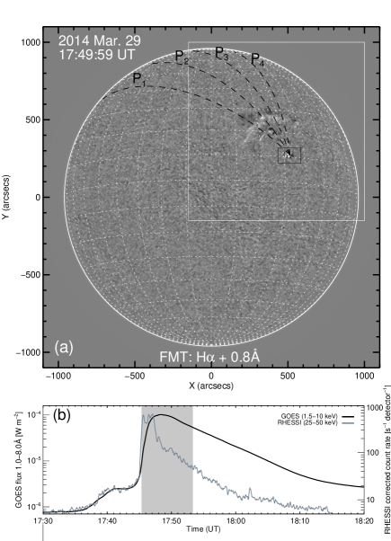
Figure 1: (a) Time-difference image of full-disk Sun at H$\alpha$ $+0.8$ Å captured by the Flare Monitoring Telescope (FMT) on 2014 March 29 at 17:49:59 UT. The image was subtracted with its precedent taken at 17:49:20 UT. The dashed black lines labeled P₁, P₂, P₃, and P₄ projected on the solar surface, outlines the paths along which the analysis of the Moreton wave is performed. The black rectangle marks the flare site, while the large white box depicts the field of view presented in Figure 2. (b) GOES X-ray emission at 1.0–8.0 Å (1.5–10 keV, black solid line) and RHESSI count rate (25–50 keV, gray solid line) of the X1.0 flare. The shaded area starting from 17:45:20 to 17:53:20 UT, denotes the time period at which the wave front is identified in our H$\alpha$ data. The animation shows time series running-difference maps of the Moreton wave at $+0.8$ and $-0.8$ Å, from 17:42 to 18:00 UT.

In Figure 1a we present a full-disk time-difference image at H$\alpha$ $+0.8$ Å (red-wing), taken by the FMT on 2014 March 29 at 17:49:20 and 17:49:59 UT. The Moreton wave is clearly seen as an arc-shaped front propagating north-east from the flare site following a trajectory of a solid angle. The great-circle dashed lines projected on the solar surface outline the paths P₁, P₂, P₃, and P₄ considered in our analysis to estimate the horizontal propagation speed of the Moreton wave and to derive the velocity amplitude in the chromosphere. Figure 1b shows the soft X-ray flux by GOES together with the hard X-ray emission by RHESSI in the energy range 25–50 keV. According to the GOES plot, which is predominantly thermal emission from the corona, the flare started at $\sim$17:35:30 UT reaching its maximum at $\sim$17:48:00 UT; whereas the RHESSI profile shows a different behavior during the impulsive and the main phase of the flare because it results from non-thermal bremsstrahlung emission. Figure 1b also indicates the time period at which the Moreton wave is observed, as represented by the gray shaded area extending from 17:45:20 to 17:53:20 UT.

The coronal wave associated with the flare under study was captured in X-ray wavelength by the X-Ray Telescope (XRT; Golub et al., 2007) on board the Hinode satellite (Kosugi et al., 2007). We use full frame images through the Ti-poly filter with a temporal resolution of $\sim$$40~{}\rm{s}$ and pixel size $\sim$$8\farcs 2~{}\rm{pixel}^{-1}$, and partial images in Al-poly and Be-thin filters with a temporal resolution and spatial sampling of $\sim$$1~{}\rm{min}$ and $\sim$$1\farcs 0~{}\rm{pixel}^{-1}$. The XRT channels are sensitive to very hot coronal plasma capable to detect emissions from $\sim$$1$ to more than $10~{}\rm{MK}$. For our study we also used extreme ultraviolet (EUV) data taken by the Atmospheric Imaging Assembly (AIA; Lemen et al., 2012) on board the Solar Dynamics Observatory (SDO; Pesnell et al., 2012). We examine the morphology and the kinematics of the coronal wave by using emission lines at 304, 211, and 94 Å, which are dominated by He ii ($\log~{}T$$\sim$$4.7$), Fe xiv ($\log~{}T$$\sim$$6.3$), and Fe xviii ($\log~{}T$$\sim$$6.8$), respectively. To characterize the local plasma responses to the EUV wave passage, we carry out differential emission measure (DEM) analysis based on the method introduced by Cheung et al. (2015). We performed DEM maps using six AIA (94, 131, 171, 193, 211, 335 Å) coronal temperature data, with full cadence ($12~{}\rm{s}$) and spatial sampling of $\sim 0\farcs 6~{}\rm{pixel}^{-1}$.

3 Wave Morphology and Kinematics

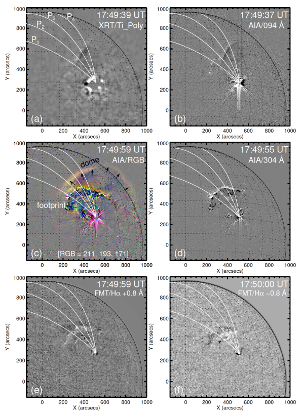
Figure 2: Coronal counterpart and Moreton wave associated with the X-class flare on 2014 March 29. The maps show different heights of the solar atmosphere, including the hotter component ($\sim$$6~{}{\rm MK}$) of corona in X-ray and 94 Å (panels a, b), intermediate component ($1$–$2~{}{\rm MK}$) as a composition of AIA 211 Å (red), 193 Å (green) and 171 Å (blue) (panel c), transition region ($\sim$$5\times 10^{4}~{}{\rm K}$) at 304 Å (panel d), and the chromosphere ($\sim$$10^{4}~{}{\rm K}$) at H$\alpha$ $\pm 0.8$ Å (panels e, f). The maps illustrate the response of the solar atmosphere to the global disturbance triggered by the large-scale wave propagation. In panel (c) the arrows highlight the dome-like expansion of the coronal wave propagating ahead of the disturbed surface (footprint). The animation includes full-disk frames of panel (c) and runs from 17:30 to 17:59 UT.

The morphology of the Moreton wave and its associated coronal counterpart is characterized by performing running-difference maps, while the kinematics is inferred from intensity variation through artificial slits and by carrying out time-distance measurements of the wave front. For the kinematics we take into account great-circle paths P₁–P₄ (shown in Figures 1, 2), projected over an angular extent on the solar surface in the wave propagation direction.

3.1 Morphology

Figure 2a-c show time-difference coronal counterpart images of the Moreton wave on 2014 March 29 in X-ray channel (Ti-poly), in EUV band at 94 Å, and a composite tri-color image (RGB = 211, 193, 171 Å), respectively. For comparison we also include time-difference images in He ii (304 Å)(panel d) and H$\alpha$ $\pm 0.8$ Å (panels e, f) to see how the different layers of the solar atmosphere respond to the effects of the wave propagation. As the temperature changes from hot to cool, the disturbance develops differently exhibiting several aspects and components of the coronal wave.

In X-ray and 94 Å (Figure 2a, b) the morphology of the coronal wave is quite similar in space and time, both representing emissions of hotter coronal plasma $>$$6.0~{}\rm{MK}$. In Figure 2c, which is a composite map of warm (211, 193 Å) and cool (171 Å) AIA channels, it can be seen a dome-shaped structure similar to a shock propagating ahead of the disturbed surface or its footprint, the latter predominantly seen in the cool channel. In much cooler line, i.e., He ii (Figure 2d) which provides diagnostics of the upper chromosphere and the transition region ($\sim$$5\times 10^{4}~{}\rm{K}$), only the footprint of the coronal wave is clearly observed as a bright arc-like feature moving towards the north-east. This thin layer possibly is strongly affected by the pressure excess created by the globally propagation shock in the corona, resulting in such an enhanced emission. On the other hand, the signature of the disturbance in the wing of the H$\alpha$ line at $\pm 0.8$ Å (Figure 2e, f) appears more diffuse and somewhat similar in morphology to that in He ii line. Naturally, the change observed in H$\alpha$ indicates an increase of the local Doppler velocity, and this aspect will be addressed in section 4.

3.2 Kinematics

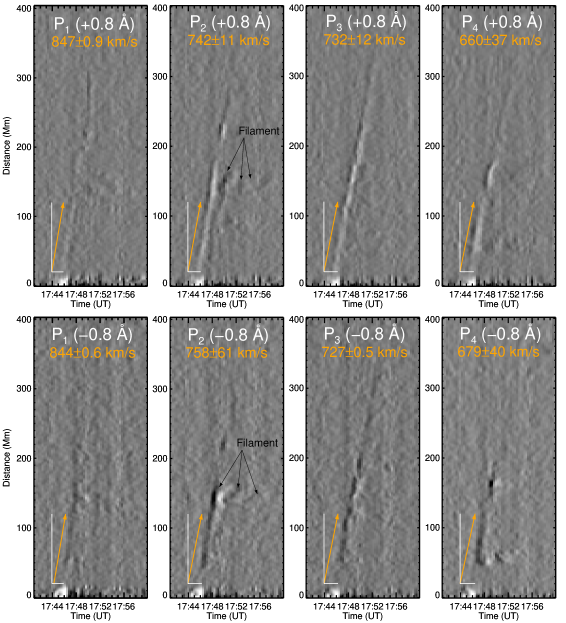
Figure 3: Time-distance diagrams of the Moreton wave obtained from running-difference images along trajectories P₁–P₄ (see panels e, f in Figure 2). The distance is expressed in megameters (Mm) starting from the flare site. The upper panels show results at H$\alpha$ $+0.8$ Å and the lower at H$\alpha$ $-0.8$ Å, wherein the orange arrows in each panel outline the earlier propagation speed of the Moreton wave. On the other hand, the black arrows in panels P₂ point-out signatures of a filament activation due to the interaction with the Moreton wave.

We performed H$\alpha$ $-0.8$ and $+0.8$ Å running-difference intensity maps in order to enhance the wave contrast. Then, we extracted the intensity variation along the slits P₁–P₄ shown in Figure 2 (panels e, f). The results are presented in Figure 3 as time-distance diagrams, in which the wave signature at H$\alpha$ $+0.8$ Å (upper panels) appears first as dark then as bright narrow stripes, while at H$\alpha$ $-0.8$ Å (lower panels) as bright and dark lanes (see also the animation of Figure 1); both displaying identical evolution and similar tendency in the propagation speed. In the time-distance diagram P₂, we can also identify signatures of the wave front interacting with quiescent filaments located in the propagation direction of the Moreton wave.

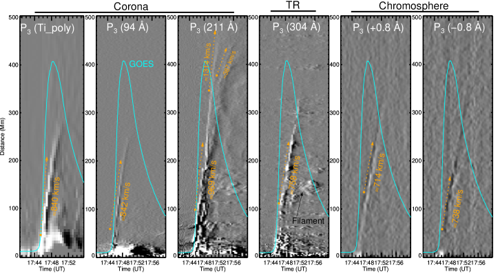
Figure 4: Time-distance diagrams of the disturbance in the corona, transition region (TR), and the chromosphere caused by the coronal wave on 2014 March 29. The intensity variation is calculated from running-difference images along trajectory P₃ shown in Figure 2. From left to right: X-ray Ti-poly filter ($\log~{}T$$\sim$$6.7$, with short time-range), EUV at 94 ($\log~{}T$$\sim$$6.8$), 211 ($\log~{}T$$\sim$$6.3$), and 304 Å ($\log~{}T$$\sim$$4.7$), and the wing of H$\alpha$ at $+0.8$, $-0.8$ Å ($\log~{}T$$\sim$$4.0$), respectively. The cyan curves are the GOES X-ray emission at the 1–8 Å channel. The time-distance diagrams reveal that the corona, transition region, and the chromosphere reacted almost simultaneously to the global scale wave propagation (see the text).

In order to compare the nature of the Moreton wave with its associated coronal wave, time-distance diagrams from EUV and X-ray observations are also performed, whose results obtained through slit P₃ (see Figure 2) are shown in Figure 4. The following characteristics can be drawn from the multiwavelength time-distance diagrams:

• Taking the starting time of the GOES flux enhancement as reference, the corona, transition region, and the chromosphere reacted almost simultaneously to the extremely large propagating disturbance in the solar atmosphere, even though we note some delay in the response of more dense layers, i.e., the transition region and the chromosphere.

• A similarity of the wave signature in terms of velocity and development is observed in H$\alpha$ and He ii (304 Å) lines, although in the latter the signature appears brighter and sharper (see also panel d in Figure 2). The enhanced emission in He ii suggests that the transition region is evidently more affected than the chromosphere by the pressure jump as a consequence of the coronal wave passage.

• Several characteristics at 211 Å are identified. The main or fast-component traveling at $\sim$$969\rm~{}{km~{}s^{-1}}$ and a slow-component moving behind it with a speed of about $387\rm~{}{km~{}s^{-1}}$. Here it is worth to add some comments on the observed features. The rapid expansion and the large propagation speed is an inherent characteristic of a fast-mode magnetosonic wave, in contrast the slower component possibly results from the deformation and restructuring of the ambient corona after the shock passage.

• In the AIA hotter channel (94 Å) and X-ray Ti-poly the wave progression behaves identically, although the intensity variation due to the disturbance lasts only for about $6$ minutes. The observed short period in these hotter channels can be ascribed to the temperature response of the instruments, since they are sensitive to hotter coronal emission well above $6~{}{\rm MK}$. Therefore, it is more likely that the 94 Å and Ti-poly filters detected mainly the hottest part of the coronal wave, possibly present during the early stage of the wave propagation.

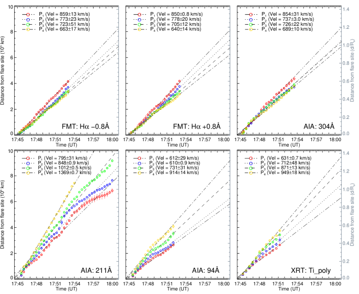
Figure 5: Time-distance plots of the Moreton wave and its associated coronal wave, measured from the flare site along paths P₁–P₄ shown in Figure 2. The top panels show H$\alpha$ $-0.8$ Å (blue-wing), H$\alpha$ $+0.8$ Å (red-wing) and He ii (304 Å), while the bottom panels show AIA 211 and 94 Å, and XRT Ti-poly filter. It is also shown the corresponding mean velocity of the wave front derived from linear-fitting, the uncertainty is estimated from the standard deviation. The right vertical axis in each panel highlighted with gray color are in units of solar radii ($1{\rm R_{s}}\approx 695,800~{}{\rm km}$).

On the other hand, we also estimated the propagating distances of the Moreton wave by tracking the leading edge of the wave front in successive images. The measurements are done along four great-circle paths (P₁–P₄), same trajectories for the time-distance diagrams, and assuming the flare site as the wave origin. The mean propagation velocity of the Moreton wave is calculated by applying the linear fitting to the time-distance plots. The results for H$\alpha$ $-0.8$ and $+0.8$ Å are presented in Figure 5 (top panels), along with the results of the wave progression derived from He ii line (304 Å). From the plots it can be seen that the Moreton wave moves faster along P₁ direction, both at H$\alpha$ $-0.8$ and $+0.8$ Å with a mean velocity of $859$ and $850~{}\rm{km~{}s}^{-1}$, respectively. It is observed that there is a tendency in the speed of the Moreton wave to slow-down as path changes from the trajectory P₁ to P₄. The derived mean velocities along paths P₂, P₃, and P₄ vary from $773$ to $663\rm~{}{km~{}s}^{-1}$ at H$\alpha$ $-0.8$ Å, and from $778$ to $640~{}\rm{km~{}s}^{-1}$ at H$\alpha$ $+0.8$ Å, respectively. The characteristics of the wave evolution at 304 Å are somewhat identical to that in H$\alpha$. Such identical features are clearly recognized by looking at the wave front speeds along paths P₁–P₄, which are comparable to the derived speeds from H$\alpha$ observations, showing also a tendency of reduction in the propagation speed as the wave moves apart from trajectory P₁ towards the northern-west. The similarities of the wave progression in He ii and H$\alpha$ lines, and also in morphology as described in section 3.1, is a clear indication that the plasma in the transition region and the chromosphere reacted in similar manner to the action of the large-amplitude disturbance in the corona.

Similar analysis is conducted using AIA coronal lines at 211 and 94 Å, as well as hotter coronal emission captured by XRT Ti-poly filter. Figure 5 (bottom panels) shows the time-distance plots derived from 211 Å, 94 Å, and Ti-poly observations, measured along paths P₁–P₄, same as for H$\alpha$ and He ii lines. It is shown that the wave in the corona develops in different manner in terms of speed and propagation direction. For example, at 211 Å the estimated values of the mean velocity extends from $795$ to $1369\rm~{}{km~{}s}^{-1}$, which increases as the wave travels in the northern-west direction (paths P₃, P₄). Same tendency shows the wave evolution at 94 Å and in Ti-poly filter, having a mean velocity from $612$ to $914\rm~{}{km~{}s}^{-1}$, and $631$ to $949\rm~{}{km~{}s}^{-1}$, respectively, although only the earlier stage of the wave front progression is identified in these hotter channels. Here it is worthwhile to point-out the following: because of the complex 3D dome-like expansion of the coronal wave and the projection effect, the results presented in the bottom panels of Figure 5 do represent the kinematics of the wave evolution at high altitudes rather than at the coronal base or the solar surface. In Table 1 a summary of the propagation speeds of the Moreton wave and the associated coronal wave calculated along the four paths are presented, including also the mean value for each wavelength domain.

Table 1: Propagation speeds of the Moreton wave and its associated coronal wave on 2014 March 29.

Path	H$\alpha$ $-0.8$ Å	H$\alpha$ $+0.8$ Å	304 Å	211 Å	94 Å	XRT/Ti-poly
P1	859 $\pm$ 13	850 $\pm$ 0.8	854 $\pm$ 30	795 $\pm$ 31	612 $\pm$ 29	631 $\pm$ 0.7
P2	773 $\pm$ 23	778 $\pm$ 20	737 $\pm$ 3.0	848 $\pm$ 0.9	610 $\pm$ 0.9	712 $\pm$ 48
P3	723 $\pm$ 51	705 $\pm$ 12	726 $\pm$ 22	1012 $\pm$ 0.5	731 $\pm$ 31	871 $\pm$ 13
P4	663 $\pm$ 17	640 $\pm$ 14	689 $\pm$ 10	1369 $\pm$ 0.7	914 $\pm$ 14	949 $\pm$ 18
Mean	754.50	743.25	751.50	1006.00	716.75	790.75

Note. — In units of ${\rm km~{}s^{-1}}$

4 Doppler Characteristics of the Moreton Wave

The Moreton wave is interpreted as a down-up swing disturbance in the chromosphere, as a result of the plasma being pushed downward by the globally expanding fast-mode wave or shock in the corona. This characteristic is regarded as compression followed by a relaxation process of the chromospheric material and induces the Doppler shift of H$\alpha$ line and brightness change in off-band images. In this section we investigate the Doppler characteristics of the Moreton wave.

4.1 H$\alpha$ intensity profiles

As a general picture, the signature of the Moreton wave in H$\alpha$ line appears as a dark front in absorption in the red-wing and as bright front in the blue-wing, followed by a wider reversed disturbance in brightening and darkening in the red and blue-wing, respectively. Since the FMT provides H$\alpha$ wing observations at two wavelength of equal distance from the line center, the absorption and brightening patterns of the wave front can be characterized by means of Doppler shift of the intensity profiles. To do so, we first normalized the H$\alpha$ $+0.8$ ($I_{red}$) and $-0.8$ Å ($I_{blue}$) intensity maps to the spatially averaged quiet-Sun level measured at disk center. Next, considering the flare site as the wave origin and the four individual trajectories (P₁–P₄), same as for the kinematics analysis described in section 3, intensity profiles as a function of distance $x$ and time $t$ are computed in red $I_{r}(x,t)$ and blue $I_{b}(x,t)$ wings by averaging the pixels intensities over consecutive areas of $\sim$$44$ arcsecs² ($1\times 11$ pixels) along each trajectory. Because the interest here is to determine the relative change of the intensity with respect to the unperturbed background, pre-event intensity profiles $I_{r}(x,t_{0})$, $I_{b}(x,t_{0})$ at 17:42:39 UT are obtained at the same positions of each corresponding trajectory, and subtracted from the intensity profiles; that is, $\Delta I_{r,b}=I_{r,b}(x,t)-I_{r,b}(x,t_{0})$.

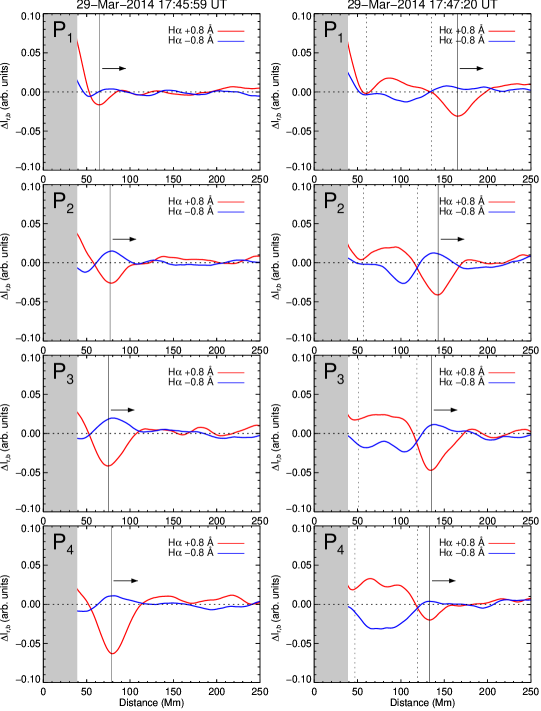
Figure 6: H$\alpha$ intensity profiles relative to the quiet-conditions at $+0.8$ Å (red-wing) and $-0.8$ Å (blue-wing), computed along trajectories P₁–P₄ at 17:45:59 and 17:47:20 UT, respectively. The gray area in each panel covers the contaminated signal by the scattered light of the flare. The profiles show perturbations as depression and enhanced patterns caused by the arrival of the coronal wave to the chromosphere (vertical solid lines). The profiles at $+0.8$ Å exhibit a strong dip (red-ward), while at the same time the profiles at $-0.8$ Å is slightly enhanced (blue-ward). This intensity changes is an indication that the H$\alpha$ spectral line is predominantly shifted red-ward. The intensity profiles also show subsequent disturbances to the wave passage (delimited by vertical dashed lines at 17:47:20 UT) showing a reversed pattern, i.e., enhancement in the red-wing and reduction of the intensity in the blue-wing. These delayed disturbances are related to the relaxation or recomposition state of the chromosphere.

In Figure 6 the obtained intensity profiles at H$\alpha$ $+0.8$ and $-0.8$ Å, computed along the four paths (P₁–P₄) for the time steps 17:45:59 and 17:47:20 UT are presented. The profiles reveal perturbations as depression and enhanced patterns caused by the arrival of the coronal wave to the chromosphere. This manifestation which is observed simultaneously as a strong depression in absorption in the red-wing and as a moderated enhancement in the blue-wing, corresponds to the downward motion of the chromospheric material caused by the collision between the coronal wave moving downward with the uppermost chromospheric layer. The characteristics observed in the profiles of H$\alpha$ wing suggests that the H$\alpha$ spectral line is predominantly shifted red-ward in the initial response. In Figure 6 it is also interesting to note that right after the downward motion the disturbed chromospheric layer exhibits a reversed pattern, i.e., brightening in the red-wing and darkening in the blue-wing (panels at 17:47:20 UT). This is because a restoration process takes place in the chromosphere after the plasma was forced to move downward, resulting in such a down-up swing disturbance.

4.2 Velocity amplitude

We further examine the strength of the disturbance in the chromosphere by computing the velocity amplitude of the chromospheric plasma. The combination of the normalized intensity maps performed previously allow us to produce Doppler signals. The following expression is applied to obtain the Doppler signal

$$DS=\frac{I_{r}(x,t)-I_{b}(x,t)}{I_{r}(x,t)+I_{b}(x,t)},$$ (1)

where $I_{r}$ and $I_{b}$ are H$\alpha$ intensity recorded at $+0.8$ (red-wing) and $-0.8$ Å (blue-wing) from the line center, respectively. Note that a positive Doppler signal corresponds to a blueshift (upward motion), and it is opposite to the convention.

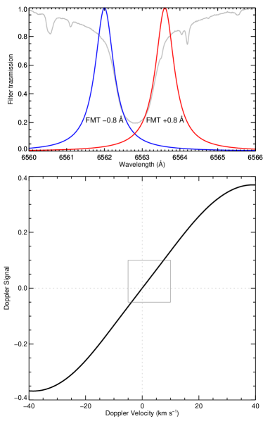
Figure 7: Upper: FMT filter-transmission profiles centered at $6562.0$ Å (blue) and $6563.6$ Å (red), respectively, both with a nominal FWHM of $0.6$ Å. The gray background profile is the atlas solar spectrum of the H$\alpha$ line normalized to the continuum. Lower: synthetic Doppler signal as a result of convolution of the FMT filter-transmission profiles with the solar spectrum. The inset box in the plot outlines the range of the Doppler signal obtained from our observation.

To quantify the Doppler signal obtained along paths P₁–P₄, we correlate them with a synthetic Doppler signal resulting from the convolution of the H$\alpha$ solar spectrum with the FMT filter-transmission profiles centered at $6562.0$ and $6563.6$ Å. Since the synthetic Doppler signal provides insights of the amount of wavelength shift $\Delta\lambda$ with respect to the core wavelength $\lambda_{0}$, we can have a direct determination of the Doppler velocity $v=(\Delta\lambda/\lambda_{0})c$, where $c$ is the speed of light. Representative profiles of the FMT filter-transmission together with the profile of the atlas solar spectrum are shown in Figure 7. Relation between the line-of-sight velocity and the Doppler signal is also shown in the lower panel of Figure 7.

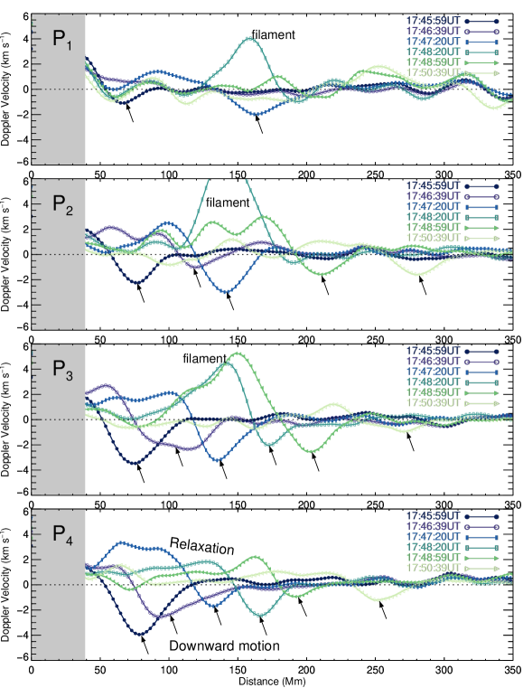
Figure 8: Doppler velocity of the Moreton wave on 2014 March 29 for six time steps along trajectories P₁–P₄. The velocity was estimated by correlating the obtained perturbation profiles with a synthetic Doppler signal (see the text). The profiles show the velocity amplitude of the moving mass at the front of the Moreton wave, wherein the arrows point-out the downward motion of the chromospheric plasma produced by the global disturbance in the corona. Also observed is a subsequent relaxation process of the chromospheric layer. At about 17:48:20 and 17:48:59 UT the profiles also exhibit strong steepness (upward motion) along paths P₁, P₂, and P₃, these features are due to the wave interaction with quiescent filaments standing in the propagation direction of the Moreton wave.

In Figure 8 we show the estimated Doppler velocity of the Moreton wave expressed as perturbation profiles, obtained along four trajectories (P₁–P₄) for six different time steps. The perturbation profiles show a clear evolution of the wave front progression, revealing downward motion and a subsequent relaxation process as upward motion of the local chromospheric plasma. This represents the velocity amplitude of the moving mass at the front of the Moreton wave. Carrying out an inspection to the perturbation profiles, we see a successive depletion (downward velocity) along P₂, P₃, and P₄ directions for the time interval between 17:45–17:50 UT, meaning that the chromospheric material is being pushed downward as the wave front hits and expands through the chromosphere. The maximum depletion caused by the wave front is observed along trajectory P₄ at 14:45:59 UT, it occurs relatively close to the source region (i.e, flare site) at a distance of $\sim$$80~{}{\rm Mm}$, reaching a highest value of about $-4~{}\rm{km~{}s}^{-1}$. At the same time and distance the perturbation profiles along P₂ and P₃ show that the plasma moves downward with a velocity of $-2.4$ and $-3.5~{}\rm{km~{}s}^{-1}$, respectively, whereas at this time the effect of the wave front along P₁ is less pronounced. Another strongest signature of plasma compression is noticed at 17:47:20 UT in P₂ and P₃ directions located at $\sim$$140~{}{\rm Mm}$ from the flare site with velocities of $-2.9$ and $-3.3~{}\rm{km~{}s}^{-1}$, respectively, and at 17:48:20 and 17:48:59 UT along trajectories P₄ and P₃ having velocities of about $-2.5$ and $-2.7~{}\rm{km~{}s}^{-1}$, respectively. It is noted that the amplitude of the velocity profiles decreases with increasing distance. For example, this effect is much more evident along P₂, P₃ and P₄ directions, suggesting that the strength of the large-amplitude coronal disturbance weakens as the time goes on.

The perturbation profiles in Figure 8 also exhibit strong steepness (upward motion) along paths P₁, P₂, and P₃, particularly at 17:48:20 and at 17:48:59 UT. These features are not due to the response of the local chromospheric plasma to the wave front passage, rather, due to the interaction with quiescent filaments laying down in the propagation direction of the Moreton wave.

4.3 Velocity map

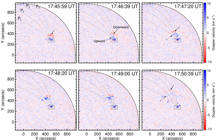
Figure 9: Doppler maps of the Moreton wave on 2014 March 29. The time period is the same to that shown in the perturbation profiles (Figure 8). The wave fronts highlighted in red and blue correspond to downward and upward motions of the chromospheric plasma (see the text). The leading edge of the Moreton wave observed in red may be related to plasma compression, while the trailing seen in blue is an indication of recovery or relaxation process of the chromosphere. The rectangles in each panel depict the flare site, and the dashed lines outlines the trajectories P₁–P₄ considered in our analysis. The online animated figure shows the Doppler characteristics of the Moreton wave from 17:44 to 18:00 UT.

The intensity maps described in section 4.1 are also used to characterize the mass motion of the local chromospheric material caused by the Moreton wave progression. Applying equation (1) we produced Doppler signal maps, then base-difference maps are obtained by subtracting a pre-event map taken at 17:42:39 UT. The subtraction essentially permit us to preserve the wave front signatures as residuals, as well as to enhance the wave contrast. Following the procedure to determine the velocity amplitude in section 4.2, by cross-correlating the base-difference maps with the synthetic Doppler signal, the line-of-sight velocity is calculated at every pixel of the map. The results are presented in Figure 9 as time-series Doppler maps, wherein it is revealed that the leading edge of the traveling wave front appears as downward motion of the chromospheric structure, followed closely by a much wider disturbance seen as the upward motion due to the restoration of the chromospheric layer. It can be noted that the wave fronts develop semicircular shapes, showing a preferential propagation direction north-east from its origin, possibly moving toward the regions of low Alfvén speed distribution (see discussion in section 6.1). As in the perturbation profiles (Figure 8), high downward velocity is observed in the initial stage of the wave propagation. It is also observed that the Moreton wave becomes progressively more diffuse and irregular, the wave signature is no longer recognized after 17:53:20 UT (see the animation of Figure 9).

5 Coronal Shock Diagnostic

In this section we focus on the characteristics of the coronal shock wave and its interaction with the underlying chromosphere. We explore the scenario in which the Moreton wave is created under the action of the MHD fast-mode wave propagation in the corona.

5.1 Corona-chromosphere interaction

In Figure 2c it is noted that the footprint of the dome-like expanding coronal wave morphologically and spatially corresponds to the wave front observed in He ii and H$\alpha$ lines (Figure 2c–f). The manifestation of the local plasma in these cooler lines is in response to the compression exerted by the downward-propagating disturbance in the corona, such as discussed in previous sections.

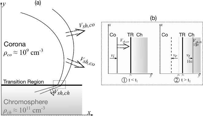
Figure 10: (a) Schematic picture of a globally propagating shock wave in the corona $V_{sh,co}$ intersecting the transition region and the chromosphere $V_{sh,ch}$. (b) Enlarged view of the interaction corona–chromosphere (dotted rectangle in panel (a), note the change of axis orientation). The illustration shows two instants of interaction: (1) shock wave propagating in the corona just before the collision with the transition region ($t<t_{1}$), and (2) subsequent period ($t>t_{1}$). At the time when the shock wave reaches the transition region, the downward motion of the plasma traveling behind the shock with a velocity $v_{i}$ (incident wave) leads to a downward shift the transition region from $y_{1}$ to $y_{2}$, this happens at $t>t_{1}$. As a consequence, the chromosphere is forced to move downward with a velocity $v_{t}$, this is the velocity amplitude of the transmitted wave from the corona to the chromosphere right after the collision and can be regarded as the velocity amplitude of the Moreton wave seen in H$\alpha$ line. Additionally, due to the density discontinuity at the boundary of corona–chromosphere, a reflected wave $v_{r}$ is also identified traveling in opposite direction in the corona.

The interaction of the corona and chromosphere can be treated as a discontinuity problem. In Figure 10a a schematic picture of a globally propagating shock in the corona intersecting the transition region and the chromosphere is presented. The illustration also shows two instants of interaction (Figure 10b), namely shock wave propagating in the corona just before the collision with the transition region ($t<t_{1}$), and the subsequent period ($t>t_{1}$). In this scheme the transition region acts as the interface layer between the corona and chromosphere, which in our analysis represents the contact discontinuity. Since the transition region is a thin layer, it is expected strong effects because the collision. At the time of shock arrival on the transition region, the downward motion of the plasma traveling behind the shock with a velocity $v_{i}$, this being the velocity amplitude of the incident wave, leads instantaneously to a downward motion of the local plasma pushing down the transition region and setting the motion in the chromosphere with a velocity $v_{t}$. This latter represents the velocity amplitude of the transmitted wave from the corona to the chromosphere right after the collision, and can be interpreted as the velocity amplitude of the chromosphere observed in H$\alpha$ line during the passage of the Moreton wave. In addition, because the sudden density jump between the corona and chromosphere, a reflected wave traveling in the corona in opposite direction is also expected and the velocity of the upward-moving plasma is denoted by $v_{r}$ in our analysis (see Figure 10b).

In one-dimensional discontinuity problem and with the aid of the conservation laws of momentum flux and energy flux, the shock wave transmission from the corona into the chromosphere can be related as follows

$$\rho_{co}(v_{i}-v_{r})c_{co}=\rho_{ch}v_{t}c_{ch}$$ (2)

$$\rho_{co}(v_{i}^{2}-v_{r}^{2})c_{co}=\rho_{ch}v_{t}^{2}c_{ch}.$$ (3)

In the above equations, $v$ is the velocity amplitude of the wave, where the subscripts denote the incident $i$, reflected $r$, and transmitted $t$ waves, as discussed above. The plasma density and the phase velocity of the MHD fast-mode wave in the corona $co$ and chromosphere $ch$ are denoted by $\rho_{co}$, $\rho_{ch}$ and $c_{co}$, $c_{ch}$, respectively. Similar to Takahashi et al. (2015) from equations (2) and (3), it is found a direct relation between the velocity amplitude of incident and transmitted waves

$$v_{i}=\left(\frac{1+\sqrt{a}}{2}\right)v_{t},$$ (4)

here $a=\rho_{ch}/\rho_{co}$ is the density ratio of chromosphere and corona. The velocity amplitude we derived from H$\alpha$ observation (Figure 8) is a direct indicator of $v_{t}$. The result of the velocity amplitude of incident wave $v_{i}$ calculated with equation (4) is listed in Table 2. The calculation is done assuming the density in the chromosphere and the corona to be $\rho_{ch}\approx 10^{11}$ and $\rho_{co}\approx 10^{9}\rm{cm^{-3}}$, respectively, and also taking as $v_{t}$ the highest downward velocity observed in the perturbation profiles of the Moreton wave.

Table 2: Velocity amplitude of incident $v_{i}$ and transmitted $v_{t}$ waves along trajectories P₁–P₄.

Time (UT)	P1			P2			P3			P4
	$v_{i}$	$v_{t}$		$v_{i}$	$v_{t}$		$v_{i}$	$v_{t}$		$v_{i}$	$v_{t}$
17:45:39	6.05	1.1		6.05	1.1		13.7	2.5		15.9	2.9
17:45:59	6.60	1.2		13.2	2.4		19.2	3.5		22.0	4.0
17:46:20	6.05	1.1		8.25	1.5		11.0	2.0		15.9	2.9
17:46:39	–	–		6.05	1.1		13.2	2.4		13.7	2.5
17:46:59	–	–		8.80	1.6		18.1	3.3		11.0	2.0
17:47:20	11.0	2.0		15.9	2.9		18.1	3.3		10.4	1.9
17:47:39	8.80	1.6		11.0	2.0		20.35	3.7		8.25	1.5
17:47:59	7.69	1.4		9.90	1.8		19.8	3.6		13.2	2.4
17:48:20	5.50	1.0		–	–		12.6	2.3		13.7	2.5
17:48:39	–	–		5.50	1.0		8.25	1.5		11.0	2.0
17:49:00	–	–		–	–		14.8	2.7		5.50	1.0
17:49:20	7.69	1.4		9.90	1.8		11.0	2.0		4.40	0.8
17:49:39	–	–		–	–		13.2	2.4		3.30	0.6
17:50:00	11.0	2.0		3.30	0.6		12.6	2.3		3.30	0.6
17:50:20	–	–		–	–		10.4	1.9		7.15	1.3
17:50:39	–	–		8.80	1.6		5.50	1.0		6.60	1.2
17:50:59	–	–		8.25	1.5		3.85	0.7		6.05	1.1

5.2 Shock strength in the corona based on the Moreton wave velocity amplitude

The purpose of this section is to show how our H$\alpha$ results can further be used to characterize the strength of the incident shock in the corona. By using the Rankine-Hugoniot relations and taking advantage of the weak shock approximation which states that the discontinuity in every quantity is small (cf. Landau & Lifshitz, 1987), that is, the shock speed is slightly larger than the sound speed, it is possible to relate the velocity amplitude of the shock in the corona to that of the velocity amplitude of the disturbance in the chromosphere, the latter being the H$\alpha$ velocity amplitude of the Moreton wave. The following expression summarize the above statements

$$v_{t}=-\frac{4}{\gamma+1}(M^{2}_{i}-1)\frac{c_{ch}}{1+c_{ch}/c_{co}},$$ (5)

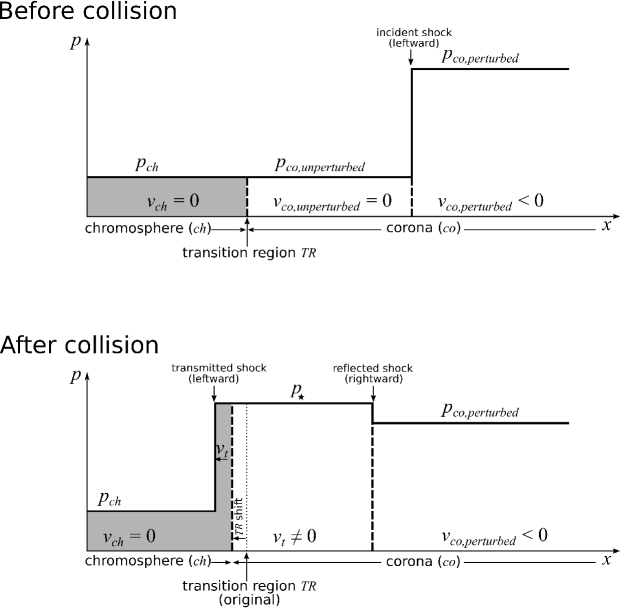
Figure 15: One-dimensional Riemann problem in hydrodynamical regime of shock interaction with the corona and chromosphere. In the illustration the transition region represents the contact discontinuity. The thick solid lines show the variation of the pressure distribution $p$ along the $x$-axis, that is, the change of the pressure in the corona and chromosphere before and after the collision of the shock with the contact discontinuity.

where $v_{t}$ is the velocity amplitude of the disturbance in the chromosphere, $M_{i}$ the Mach number of the incident shock in the corona, and $c_{ch}$, $c_{co}$ are the propagation speed of the shock in the chromosphere and corona, respectively. The derivation of this equation is presented in the Appendix A (see also Figure 15). Equation (5) allows to estimate the Mach number of the shock in the corona for a given value of the H$\alpha$ velocity amplitude.

Let us discuss equation (5) in more detail. Under the weak shock approximation, the propagation speed of the shock in the corona is the sound speed, under this condition the situation in the chromosphere may be also the same. For example, for a typical temperature in the chromosphere $T\approx 10^{4}~{}{\rm K}$, one finds the sound speed $c_{s}=\sqrt{(\gamma~{}k~{}T)/m_{p}}\approx 10~{}{\rm km~{}s^{-1}}$, where $k$ is the Boltzmann constant, $m_{p}$ the proton mass, and $\gamma$ the adiabatic index of the gas. In weak shock events this sound speed would be comparable to the speed of the shock in the chromosphere, as we noted above. Furthermore, because the sound speed in the corona is about one order of magnitude larger than that in the chromosphere, or even more, the term $c_{ch}/c_{co}$ in the equation can be neglected.

Taking into account the above considerations and making use of the derived velocity amplitude of the Moreton wave $v_{t}$ along with the adiabatic index $\gamma=5/3$, equation (5) can be now evaluated. The results are shown in Table 3. We stress that the calculation presented here is in one-dimensional regime and a pure hydrodynamic approach, no magnetic field effect is being considered. A future work will be devoted on this calculation including much more details.

Table 4: Mach number of the incident shock in corona along trajectories P₁–P₄, based on the Moreton wave velocity amplitude.

Time (UT)	P1	P2	P3	P4
17:45:39	1.04	1.04	1.08	1.09
17:45:59	1.04	1.08	1.11	1.12
17:46:20	1.04	1.05	1.06	1.09
17:46:39	–	1.04	1.08	1.08
17:46:59	–	1.05	1.10	1.06
17:47:20	1.06	1.10	1.11	1.06
17:47:39	1.05	1.07	1.11	1.05
17:47:59	1.05	1.06	1.11	1.08
17:48:20	1.03	–	1.07	1.08
17:48:39	–	1.03	1.05	1.06
17:49:00	–	–	1.08	1.03
17:49:20	1.04	1.06	1.06	1.03
17:49:39	–	–	1.08	1.02
17:50:00	1.06	1.02	1.07	1.02
17:50:20	–	–	1.06	1.04
17:50:39	–	1.05	1.03	1.04
17:50:59	–	1.05	1.02	1.03

Note. — ($v_{i}$ and $v_{t}$ in units of ${\rm km~{}s^{-1}}$). The blanks indicate the time where it is not possible to determine signatures of downward motion in the H$\alpha$ perturbation profiles.

Note. — The blanks indicate the time where it is not possible to determine signatures of downward motion in the H$\alpha$ perturbation profiles.

5.3 Shock characteristics in the corona

According to the MHD shock theory the jump relation that describes an oblique shock is defined as (Priest, 2000)

$$(v_{1}^{2}-Xv_{A1}^{2})^{2}\{Xc_{s1}^{2}+\frac{1}{2}v_{1}^{2}\cos^{2}\theta(X(\gamma-1)-(\gamma+1))\}$$

$$+\frac{1}{2}v_{A1}^{2}v_{1}^{2}\sin^{2}\theta~{}X$$

$$\times\{(\gamma+X(2-\gamma))v_{1}^{2}-Xv_{A1}^{2}((\gamma+1)-X(\gamma-1))\}$$

$$=0,~{}~{}~{}~{}$$ (6)

where $X\equiv\rho_{2}/\rho_{1}$ is the compression ratio or density jump at the front of the shock, $\theta$ is the angle between the upstream magnetic field and the shock normal, $c_{s}$ and $v_{A}$ are the sound and Alfvén speeds, respectively. Taking for the adiabatic index $\gamma=5/3$ and the sound speed $c_{s}^{2}=(\gamma\beta/2)v_{A}^{2}$, equation (6) can be rewritten in terms of the Alfvén Mach number $M_{A}$ as follows (see the Appendix B, also Vršnak et al., 2002b)

$$(M_{A1}^{2}-X)^{2}\{5\beta X+2M_{A1}^{2}\cos^{2}\theta(X-4)\}+M_{A1}^{2}\sin^{2}\theta~{}X$$

$$\times\{M_{A1}^{2}(5+X)+2X(X-4)\}=0.~{}~{}~{}~{}$$ (7)

Equation (7) depends on the inclination $\theta$, the compression ratio $X$, and also on the ratio of the plasma to the magnetic field pressure $\beta$. Under the assumption that the proton number density $n$ of the coronal emitting plasma is constant along the line-of-sight, the compression ratio may roughly be estimated from the emission measure $EM\simeq n^{2}l$, where $l$ is the depth of the emitting plasma along the line-of-sight. Since the coronal mass density is $\rho\simeq nm_{p}$, $m_{p}$ being the proton mass, it is reliable to express the following quantities as ${EM_{2}}/{EM_{1}}={\rho_{2}^{2}}/{\rho_{1}^{2}}$, here the subscripts 1 and 2 denote the emission measure and mass density ahead of and behind the shock front, respectively, and we assume that $l$ is common between them, therefore we can write

$$X\equiv\frac{\rho_{2}}{\rho_{1}}=\sqrt{\frac{EM_{2}}{EM_{1}}}.$$ (8)

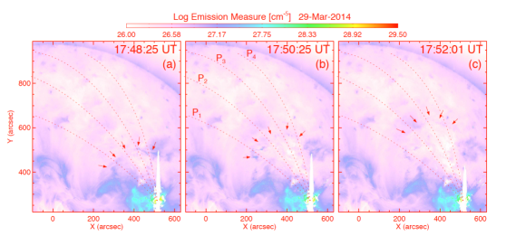
Figure 11: Differential emission measure (DEM) maps showing three instants of the coronal wave on 2014 March 29. We used the method of Cheung et al. (2015), which enabled us to obtain DEM maps for a set of temperature bins. The panels show DEM solutions for a temperature range of $6.1\leq\log T/{\rm K}\leq 6.4$ (see the text), wherein the manifestation of wave propagation (arrows) clearly can be distinguished traveling northeast. Based on these results, we calculate DEM perturbation profiles along trajectories P₁ to P₄ (dashed lines), which were used to derive the compression ratio $X$ presented in Figure 12.

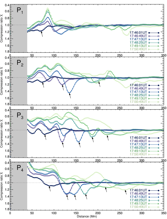
Figure 12: Compression ratio $X$ estimated from DEM maps along trajectories P₁–P₄ shown in Figure 11. We obtained the total emission measure by integrating over a temperature range the DEM perturbation profiles, then equation (8) is applied to estimate the compression ratio (see the text). The pre-shocked emission measure $EM_{1}$ in equation (8) is that resulting from DEM map at 17:42:37 UT. The compression ratio profiles along each trajectory correspond to the nearest time interval of the Moreton wave velocity amplitude presented in Figure 8. Note that the vertical axes are inverted, this for a better comparison of the observed characteristics (arrows) with those in the Moreton wave perturbation profiles. The online animation presents a synchronized time evolution of the compression ratio and the Moreton wave velocity amplitude along trajectory P₃, extending from 17:42 to 17:51 UT.

The emission measure is estimated from AIA observations by applying DEM inversion method of Cheung et al. (2015). As a first step we constructed DEM maps for a set of 21 temperature bins, spanning $\log T/{\rm K}=5.7$ to $7.7$. We notice that DEM solutions for $\log T/{\rm K}<6.1$ do not show clearly signatures of the wave front progression, and although solutions for $\log T/{\rm K}>6.4$ exhibit signs of the wave front, it is greatly influenced by the scattered light of the flare. Since our interest is to trace the wave propagation, we restrict the temperature grid to $6.1\leq\log T/{\rm K}\leq 6.4$, at which the coronal wave front in DEM maps is best observed (see Figure 11). Next, considering four trajectories from the flare site (P₁–P₄), same as for the Moreton wave (see section 4), we proceed to obtain perturbation profiles by spatially averaging the DEM solutions along each trajectory shown in Figure 11. Lastly, the computed DEM perturbation profiles in the temperature range $6.1\leq\log T/{\rm K}\leq 6.4$ were integrated to obtain the total emission measure $EM$, which enabled us to derive the compression ratio $X$ by applying equation (8). It should be noted that for the calculation of the compression ratio we have considered as $EM_{1}$ in equation (8) a pre-shocked emission measure at 17:42:37 UT. Figure 12 shows the obtained compression ratio distribution along four trajectories, corresponding to the nearest time interval of the Moreton wave velocity amplitude shown in Figure 8.

On the other hand, the pre-shocked plasma temperature in the corona was constrained by applying the XRT filter ratio method (Narukage et al., 2011) on two pairs of filters (Al-poly/Be-thin), which results in $T_{1}\simeq 2.5{\rm~{}MK}$. Considering this value the sound speed in the corona $c_{s}=\sqrt{(\gamma~{}k~{}T_{1})/m_{p}}$ is $185{\rm~{}km~{}s^{-1}}$. Moreover, based on XRT Ti-poly observations the speed of the fast-mode wave in the corona can be assumed to be $c_{f}\simeq 790~{}{\rm km~{}s^{-1}}$, corresponding to the mean value of the speeds along trajectories P₁–P₄ (see Table 1). In the case of perpendicular wave propagation ($\theta=90\arcdeg$), the Alfvén speed in the corona is defined as $v_{A}=\sqrt{c_{f}^{2}-c_{s}^{2}}$, which yields $v_{A}=768~{}{\rm km~{}s^{-1}}$. Finally, taking the obtained results of the sound speed and the Alfvén speed, the plasma-to-magnetic pressure ratio in the corona is estimated as $\beta=0.06$, allowing us now to evaluate equation (7) and find solutions for the Alfvén Mach number $M_{A}$ for given values of the inclination $\theta$. Furthermore, if we assume the velocity of the shock in the corona to be $v_{sh}$, it is straightforward to relate the Alfvén Mach number $M_{A}=v_{sh}/v_{A}$ along with the sound speed $c_{s}$ to the fast-mode (or fast magnetosonic) Mach number $M_{f}=v_{sh}/c_{f}$. Again, for a perpendicular case the following relation holds

$$M_{f}=\frac{M_{A}}{\sqrt{1+\gamma\beta/2}}.$$ (9)

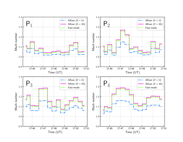
Figure 13: Alfvén and fast-mode Mach numbers of the coronal wave on 2014 March 29 along trajectories P₁–P₄. The Alfvén Mach number is based on the solution of equation (7) using the compression ratio derived from differential emission measure. The profiles in blue and magenta show solutions for horizontal ($\theta=0\arcdeg$) and perpendicular ($\theta=90\arcdeg$) shock propagation cases, respectively. For the calculation we take the highest values of the compression ratio profiles in each trajectory, those that are closely connected to the positions of large downward motion of the Moreton wave. On the other hand, the fast-mode Mach number (green profiles) are solutions of equation (9) taking the results of the Alfvén Mach number for the perpendicular case.

In Figure 13 solutions of equation (7) for the Alfvén Mach number are presented. The calculations are done by considering two scenarios of shock propagation: horizontal ($\theta=0\arcdeg$) and perpendicular ($\theta=90\arcdeg$) (see the Appendix B), and taking the highest possible values of the compression ratio profiles in the four trajectories; those that are closely connected to the positions of the most prominent downward motion of the Moreton wave at each instance. Figure 13 also compares the fast-mode Mach number estimated with equation (9), this based on the Alfvén Mach number derived for the perpendicular case.

6 Discussion

6.1 Morphology and propagation speed of the Moreton wave

The Moreton wave on 2014 March 29 has brought interesting insights into our picture of chromospheric disturbances associated with flares. Thanks to the multiwavelength coverage it was possible to reveal details of this wavelike phenomenon happening in the chromosphere in conjunction with its coronal counterpart. It is not surprising that the derived propagation speed of the Moreton wave is comparable to that of the propagation speed of the coronal wave obtained from AIA and XRT observations, and the morphology of the wave front seen in the chromosphere also shows a good correspondence in space and time with the footprints of the expanding dome-like structure in the corona (Figure 2). This scenario further confirms that Moreton waves are the chromospheric manifestation of an MHD fast-mode shock wave traveling through the corona, as theoretically anticipated by Uchida (1968). Furthermore, the multiwavelength time-distance diagrams presented in Figure 4 show that each region of the solar atmosphere reacts and evolves quasi-simultaneously, implying that a globally propagating shock in the corona is the triggering source of the observed disturbances.

We found that the mean velocity of the Moreton wave varies depending on the wave propagation direction (Figure 5, top panels). Similar behavior is also observed in the coronal wave propagation speed (Figure 5, bottom panels), although in the latter case the situation is much more complex due to the 3D expansion and the projection effect. The difference of the propagation velocity along the analyzed trajectories can be attributed to the plasma condition and the inhomogeneous topology through which the wave propagates. In the solar atmosphere both the density and the magnetic field change considerably along the vertical direction, i.e., the density starts to decrease rapidly in the low corona, while the magnetic field drops much faster in the outer corona. This aspect determine the ambient Alfvén speed, which is an important parameter to characterize wave propagation in the corona and their subsequent effects. The studied Moreton wave also exhibits a confined propagation direction to a certain sector, i.e., north-east from the flare site. The reason of this confinement is because the MHD fast-mode wave cannot re-enter the chromosphere in directions in which strong magnetic field does exist. Strong magnetic field also implies that high Alfvén velocity distribution dominates these regions; and because the wave front tends to propagate avoiding strong magnetic regions, the wave energy flux concentrates in directions of low Alfvén velocity. Therefore, the occurrence of this condition in the low corona favors to the appearance of the Moreton wave in a restricted direction (cf. Uchida et al., 1973). Indeed, the Moreton wave on 2014 March 29 was directed towards non-magnetic or weak-field regions, i.e., high latitudes from the flare site, but not in opposite direction or towards the equatorial zone, places where high concentration of magnetic field could exist because of the presence of magnetic structures and some active regions. Zhang et al. (2011) based on the analysis of a set of Moreton waves, also showed that the waves tend to propagate within a boundary of weak magnetic field regions.

6.2 Doppler velocity of the Moreton wave

The quantitative results of the perturbation in the chromosphere presented as Doppler velocity in Figure 8, provides a direct sign of the coronal disturbance exerted into the chromosphere. The perturbation profiles show that the arrival of the coronal wave to the chromosphere produces disturbances along the four trajectories (P₁–P₄). However, its effect differs from one trajectory to another, and there is no a clear correlation among them in terms of amplitude as a function of distance and time. The wave propagation along path P₁ causes a very weak disturbance, whereas in P₂, P₃, and P₄ directions the disturbances becomes gradually much more significant. It is also noted that in the earlier stage, i.e., at 17:45:59 – 17:47:20 UT, highest downward velocity is observed particularly along P₂, P₃ and P₄ trajectories, later on the velocity amplitude decreases. The difference of the velocity amplitude we found along each trajectory may be a consequence of the non-homogeneous layer (density and field strength) over which the wave propagates in the corona. In addition, because the downward component of the coronal wave interacts with a much more dense layer, i.e., the chromosphere, most of its energy is reflected back into the corona and only a small fraction of it is able to reach deeper layers triggering disturbances with strong effect in some localized regions, such as observed in the H$\alpha$ perturbation profiles. Furthermore, the wave fronts seen in the Doppler maps (see Figure 9 and the associated movie) progressively becomes wider and diffuse. This is indicative that the strength of the disturbance in the corona gets weaker at far distances from the source, meaning that some dissipative process undergoes and as a result damping of the wave takes place, similar to the perturbation profiles. Vršnak et al. (2016) in their simulation results showed that after a certain time the velocity amplitude of the chromospheric disturbance develops a small amplitude. The authors also reproduced the restoration process of the perturbed plasma, consistent with our observational results.

6.3 Characteristics of the coronal wave based on H$\alpha$ observation

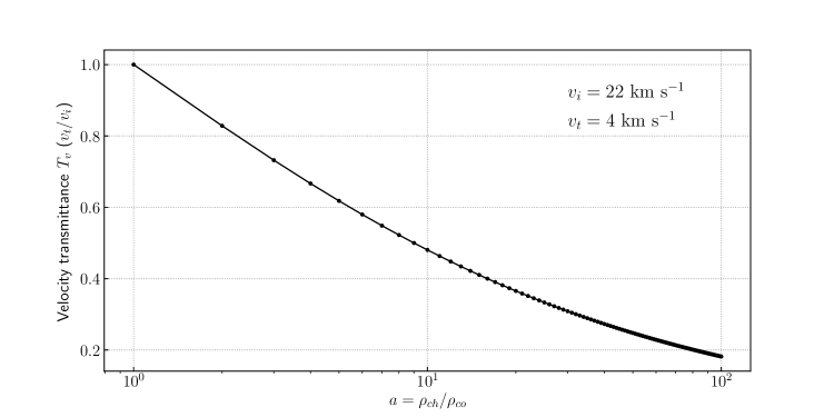
Figure 14: Velocity transmittance $T_{v}$ defined as the ratio of the velocity amplitude of transmitted $v_{t}$ and incident $v_{i}$ waves. This provides clues on how much fraction of the plasma velocity in the corona is transferred to the chromosphere during the shock wave propagation. For illustration, the density jump $a$ extends from $1$ to $100$, and we take $v_{t}=4~{}{\rm km~{}s^{-1}}$ and $v_{i}=22~{}{\rm km~{}s^{-1}}$ corresponding to the trajectory P₄ at 17:45:59 UT (see Table 2). In the plot it can be seen that as $a$ increases $T_{v}$ is significantly reduced.

We have shown in section 5.1 that the MHD linear theory and the H$\alpha$ velocity amplitude of the Moreton wave, this latter interpreted as the velocity amplitude $v_{t}$ of the transmitted wave from the corona to the chromosphere, allowed us to infer the velocity amplitude $v_{i}$ of the incident wave in the corona under the assumption that the density ratio of chromosphere and corona is $a\approx 100$. It is important to emphasize that our calculation of $v_{i}$ should be understood as the associated counterpart of $v_{t}$ acting at the base of the corona. Taking the ratio of the velocity amplitude of transmitted and incident waves, we define the velocity transmittance $T_{v}=v_{t}/v_{i}$. This provides clues on how much fraction of the plasma velocity in the corona is transferred to the chromosphere when the shock front surpasses a specific location of the dense chromospheric layer. To illustrate this point, we assume that $a$ extends from $1$ to $100$, and also we take $v_{t}=4~{}{\rm km~{}s^{-1}}$ and $v_{i}=22~{}{\rm km~{}s^{-1}}$, corresponding to the derived values along path P₄ at 17:45:59 UT (see Table 2). It is shown in Figure 14 that as $a$ increases $T_{v}$ is significantly reduced, so the effect of the density increase, e.g., corona–chromosphere density jump, plays an important role. Takahashi et al. (2015) (in their Figure 11) also found a similar tendency of velocity transmittance from one-dimensional simulation of shock transmission to a prominence.

From our findings we can further speculate that a wave traveling downward at the base of the corona with a velocity $\gtrsim 10~{}{\rm km~{}s^{-1}}$, this being the mean velocity amplitude of the incident wave calculated along trajectories P₃ and P₄ in Table 2, could be able to produce a noticeable disturbance in the chromosphere. We are aware that this is simply based on linear analytic solution, however, if the amplitude of the disturbance is so small, such as in the limit corona–chromosphere, the linear theory is applicable. Harra et al. (2011) and Veronig et al. (2011), based on Hinode/EIS observation of a coronal wave on 2011 February 16, reported a downward motion of the plasma in the corona with a velocity of about $20~{}{\rm km~{}s^{-1}}$. The authors argued that the coronal wave pulse moving with such a speed was not strong enough to produce disturbances in the chromosphere. Indeed there was no Moreton wave, but activation of filaments in H$\alpha$ line were identified associated with the referred coronal wave (cf. Cabezas et al., 2017). It should be mentioned that the reported downward motion was observed in Fe xii and Fe xvi spectral lines, which provide plasma diagnostics of coronal emission at $\log T/K\gtrsim 6.1$, whose formation region is believed to be located at low or mainly at intermediate corona, and it is likely that plasma moving downward with $20~{}{\rm km~{}s^{-1}}$ at such a place could not effectively travel deeper to overcome the inert chromosphere and produce a Moreton wave.

6.4 Shock strength in the corona based on DEM analysis

The compression ratio profiles shown in Figure 12 reveal that the coronal wave propagates by exhibiting an irregular pattern along the different trajectories. It is found that the compression ratio, which is directly related to the shock strength, varies non-uniformly as a function of distance and time. On the basis of the shock wave theory, the propagation and strength of the shock in the corona is governed by the action of the magnetic field and the ambient Alfvén speed distribution, and in the absence of strong magnetic field high compression ratio is expected. Therefore, the large values of the compression ratio observed along P₂, P₃, and P₄ directions, implying high Mach number (see Figure 13), suggests that these locations are more likely weak magnetic field regions. Consequently, the shock traveling along these directions could produce strong compression, resulting in relatively large amplitude chromospheric disturbance. In fact, strong downward motions in the chromosphere are observed along the referred trajectories. This can be seen by comparing Figures 8 and 12, in which highest values of the compression ratio along trajectories P₂, P₃, and P₄, approximately match in distance and time to the large downward motion caused by the Moreton wave (see the animation of Figure 12). Of course, a comparison between the compression ratio and the velocity amplitude of the Moreton wave cannot be done directly, since the compression ratio based on DEM ($6.1\leq\log T/{\rm K}\leq 6.4$) is a plasma diagnostic of the wave traveling above the low corona, we are missing information of the plasma in the lowest-part of the corona. Nevertheless, the compression ratio profiles and the velocity amplitude of the Moreton wave show a good correspondence.

The disturbance created by the wave propagation would also result in the increase of the local plasma temperature. As we pointed out in section 5.3, DEM solutions for $\log T/{\rm K}<6.1$ do not show clear signs of the wave propagation. In contrast, at much higher temperature range the disturbance seen as emission enhancement becomes more noticeable. Similar findings from DEM analysis of coronal waves were also reported by Vanninathan et al. (2015) and Liu et al. (2018). The emission increasing at high temperatures is an indication of plasma heating, enhanced locally due to plasma compression as a result of the wave propagation. The heating effect also causes intensity variation of much cooler emission lines. For example, at AIA 171 Å ($\log T$$\sim$$5.8$) coronal dimming (not shown here) is observed at the place of the wave front as a consequence of the plasma being heated to much higher temperatures (e.g., Wills-Davey & Thompson, 1999; Delannée, 2000; Liu et al., 2010; Nitta et al., 2013; Liu et al., 2018).

7 Summary and Conclusion

In this work we have studied in detail the Moreton wave on 2014 March 29 and its associated coronal counterpart. We combined multiwavelength observations, including H$\alpha$ $\pm 0.8$ Å, He ii ($304$ Å), coronal emission lines from AIA, and Hinode X-ray. This data set permitted us to further understand the nature of a globally wave propagation and their subsequent effects at different layers of the solar atmosphere. Such a global effect is clearly evidenced in Figure 4, wherein it is observed how the corona, transition region, and the chromosphere reacted to the large-scale disturbance. It is also noted a co-spatial evolution of the wave in the corona and the Moreton wave in the transition region and the chromosphere, particularly in the initial stage of the propagation, thus confirming a common origin.

Thanks to the observations in the wing of the H$\alpha$ line performed by the FMT, we discussed the Doppler characteristics of the Moreton wave. We have shown that it is possible to quantify the downward motion of the chromospheric material traveling at the front of the Moreton wave. The plasma at this location attains a maximum velocity of about $4~{}{\rm km~{}s^{-1}}$, which corresponds to the velocity amplitude of chromospheric motion associated with the Moreton wave. Our findings also showed that the chromospheric disturbance develops non-uniformly in terms of amplitude along the analyzed trajectories (see Figure 8). Furthermore, with the aid of the MHD linear theory we also related our results of the Moreton wave velocity amplitude with that of the plasma velocity in the corona, allowing us to infer the velocity amplitude of the incident wave from the corona to the chromosphere. Additionally, we showed that by using the weak shock approximation in conjunction with the velocity amplitude of the Moreton wave, the Mach number of the incident shock in corona could be estimated and obtained a consistent result with the AIA analysis. Very recently Long et al. (2019) attempted to characterize the perturbation caused by the Moreton wave studied in this paper, but the authors used H$\alpha$ line core observations only, in which the signature of the perturbation cannot easily be distinguished.

The compression ratio analysis led us to conclude that the wave in the corona develops in a complex manner. This may depend on the conditions in which the wave propagates through. As we noticed in Figure 12, the compression ratio profiles vary as a function of distance, time, and also from one trajectory to another. This aspect also has a direct consequence in the change of the Alfvén and fast-mode Mach numbers, such as presented in Figure 13. As for the Mach number, the values we calculated (i.e., $M_{A}\approx$1.06–1.28 and $M_{f}\approx$1.05–1.27) should be understood as representing the strength of the shock in a confined region of the solar corona, since we restricted the compression ratio analysis to a DEM temperature range $6.1\leq\log T/{\rm K}\leq 6.4$, the missed lowest-part of the corona should be taken into account for further conclusions.

Finally, an extension of the present work will be important especially focusing on the Doppler characteristics of the Moreton wave, a topic which is not fully understood and scarcely explored. More studies will help us to advance and clarify the direct connection between the downward propagating component of the coronal wave and the chromospheric reaction leading to a Moreton wave. To this end, a combination of numerical experiments and observational results will be crucial. As for the observational matter, it will be further constrained with the Solar Dynamics Doppler Imager (SDDI; Ichimoto et al., 2017), now in operation on SMART telescope at Hida Observatory, Kyoto University, which provides high resolution filtergrams with the spectral profiles in a wide spectral window around the H$\alpha$ line center.

Appendix A Mach number in terms of the Moreton wave velocity amplitude

In this section we present the derivation of equation (5) introduced in section 5.2. Here we discuss the one-dimensional Riemann problem in hydrodynamical regime (Landau & Lifshitz, 1987) based on the weak shock approximation. The three-dimensionality and the magnetohydrodynamic effects are not considered.

Figure 15 shows an illustration of shock interaction before and after the collision with the contact discontinuity (transition region). In the scheme the solid thick line represent the variation of the pressure $p$ along the $x$-axis. Before the collision, the initial pressure distribution in the chromosphere and corona are in equilibrium ($p_{0}=p_{ch}=p_{co}$, $v_{ch}=v_{co}=0$) and is separated by the contact discontinuity. In our analysis the coronal shock (incident shock) propagates from right to left, where its downstream region is characterized with enhanced pressure $p^{\prime}_{co}=p_{co,perturbed}$ and velocity $v^{\prime}_{co}=v_{co,perturbed}$. Note that in the following we take the direction from the chromosphere to corona as positive direction, and thus, $v^{\prime}_{co}=v_{co,perturbed}<0$. After the collision of the incident shock with the contact discontinuity, the pressure and the velocity distribution can be divided into three regions: $p=p_{0}$, $v=0$ in the leftmost region; $p=p^{\prime}_{co}$, $v=v^{\prime}_{co}$ in the rightmost; and an intermediate region characterized with $p_{\star}$ and $v_{t}$ (lower panel in Figure 15).

The Rankine-Hugoniot relations tells us about the jump conditions at the incident $i$, transmitted $t$, and reflected $r$ shocks, in which the Mach number of each shock can be expressed respectively as

$$M_{i}^{2}=1+\frac{\gamma+1}{2\gamma}\left(\frac{p^{\prime}_{co}}{p_{0}}-1\right),\quad M_{t}^{2}=1+\frac{\gamma+1}{2\gamma}\left(\frac{p_{\star}}{p_{0}}-1\right),\quad M_{r}^{2}=1+\frac{\gamma+1}{2\gamma}\left(\frac{p_{\star}}{p^{\prime}_{c0}}-1\right)$$ (A1)

$$0-v^{\prime}_{co}=\frac{2c_{co}}{\gamma+1}\frac{M_{i}^{2}-1}{M_{i}},\quad 0-v_{t}=\frac{2c_{ch}}{\gamma+1}\frac{M_{t}^{2}-1}{M_{t}},\quad(-v^{\prime}_{co})-(-v_{t})=\frac{2c^{\prime}_{co}}{\gamma+1}\frac{M_{r}^{2}-1}{M_{r}}$$ (A2)

where $c_{co}=\sqrt{\gamma p_{0}/\rho_{co,unperturbed}}$, $\quad c_{ch}=\sqrt{\gamma p_{0}/\rho_{ch,unperturbed}}$, $\quad c^{\prime}_{co}=\sqrt{\gamma p^{\prime}_{0}/\rho_{co,perturbed}}$ ; therefore

$$-v^{\prime}_{co}=\frac{2c_{co}}{\gamma+1}\frac{M^{2}_{i}-1}{M_{i}}=\frac{2c^{\prime}_{co}}{\gamma+1}\frac{\frac{\gamma+1}{2\gamma}\left(\frac{p_{\star}}{p^{\prime}_{co}}-1\right)}{\sqrt{1+\frac{\gamma+1}{2\gamma}\left(\frac{p_{\star}}{p^{\prime}_{co}}-1\right)}}+\frac{2c_{ch}}{\gamma+1}\frac{\frac{\gamma+1}{2\gamma}\left(\frac{p_{\star}}{p_{co}}-1\right)}{\sqrt{1+\frac{\gamma+1}{2\gamma}\left(\frac{p_{\star}}{p_{co}}-1\right)}}.$$ (A3)

Because $p^{\prime}_{co}$ can be described with $p_{0}$ for given $M_{i}$ in equation (A1), the second equality of equation (A3) determines the dependence of $p_{\star}$ on $p_{0}$ and $M_{i}$, and thus, $M_{t}$ and $v_{t}$ can be also determined as a function of $p_{0}$ and $M_{i}$ by equation (A2). Particularly, for weak shock $M^{2}_{i}-1\ll 1~{}(\Leftrightarrow\delta:=p^{\prime}_{co}/p_{0}-1\ll 1)$, $\delta_{\star}:=p_{\star}/p_{0}-1\ll 1$, then we have

$$M^{2}_{i}-1\approx\frac{\gamma+1}{2\gamma}\delta,\quad\frac{\frac{p_{\star}}{p^{\prime}_{co}}-1}{\sqrt{1+\frac{\gamma+1}{2\gamma}\left(\frac{p_{\star}}{p^{\prime}_{co}}-1\right)}}\approx\delta_{\star}-\delta,\quad\frac{\frac{p_{\star}}{p_{0}}-1}{\sqrt{1+\frac{\gamma+1}{2\gamma}\left(\frac{p_{\star}}{p_{0}}-1\right)}}\approx\delta_{\star}.$$ (A4)

The previous statements lead us to express equation (A3) as

$$\frac{c_{co}}{\gamma}\delta\approx\frac{c_{co}}{\gamma}(\delta_{\star}-\delta)+\frac{c_{ch}}{\gamma}\delta_{\star},$$ (A5)

which is reduced to

$$\delta_{\star}=\frac{2}{1+c_{ch}/c_{co}}\delta.$$ (A6)

Furthermore, we can relate the Mach numbers of incident and transmitted shock as

$$M^{2}_{t}-1\approx\frac{2}{1+c_{ch}/c_{co}}(M^{2}_{i}-1),$$ (A7)

then from equations in (A2) we arrive to an expression that relates $v_{t}$ to the Mach number of transmitted and incident shocks from the corona

$$v_{t}\approx-\frac{2c_{ch}}{\gamma+1}(M^{2}_{t}-1)\approx-\frac{4c_{ch}}{\gamma+1}(M^{2}_{i}-1)\frac{1}{1+c_{ch}/c_{co}}.$$ (A8)

It should be noted again that $v_{t}$ is the velocity in the intermediate region which appears after the collision between the shock and the contact discontinuity (Figure 15). In other words, the contact discontinuity starts to move leftward with the velocity of $v_{t}$, affecting also the chromosphere and could be observed as the Doppler shift of H$\alpha$ line.

Appendix B Alfvén Mach number from oblique shock jump relations

Here we show the solution of equation (6) in terms of Alfvén Mach number. As in section 5.3 the following notation describes an oblique shock (Priest, 2000)

$$(v_{1}^{2}-Xv_{A1}^{2})^{2}\{Xc_{s}^{2}+\frac{1}{2}v_{1}^{2}\cos^{2}\theta(X(\gamma-1)-(\gamma+1))\}+\frac{1}{2}v_{A1}^{2}v_{1}^{2}\sin^{2}\theta X$$

$$\times\{(\gamma+X(2-\gamma))v_{1}^{2}-Xv_{A1}^{2}((\gamma+1)-X(\gamma-1))\}=0.$$ (B1)

Assuming the adiabatic index $\gamma=5/3$ and expressing the sound speed as $c^{2}_{s}=(\gamma\beta/2)v^{2}_{A}$, the first and second part of equation (B9) can be written respectively as

$$\frac{1}{3}(v_{1}^{2}-Xv^{2}_{A1})^{2}\left\{\frac{5}{2}X\beta v_{A1}^{2}+v_{1}^{2}\cos^{2}\theta(X-4)\right\}+\frac{1}{3}v_{A1}^{2}v_{1}^{2}\sin^{2}\theta X$$

$$\times\left\{\frac{v_{1}^{2}}{2}(5+X)+v_{A1}^{2}X(X-4)\right\}=0,$$ (B2)

and multiplying by $1/v_{A1}^{2}$ allows to express in terms of Alfvén Mach number $M_{A1}$

$$(v_{1}^{2}-Xv_{A1}^{2})^{2}\left\{5\beta X+2M_{A1}^{2}\cos^{2}\theta(X-4)\right\}+v_{A1}^{2}v_{1}^{2}\sin^{2}\theta X$$

$$\times\left\{M_{A1}^{2}(5+X)+2X(X-4)\right\}=0.$$ (B3)

Finally, after some algebraic procedures one arrives to the following solution

$$(M_{A1}^{2}-X)^{2}\left\{5\beta X+2M_{A1}^{2}\cos\theta^{2}(X-4)\right\}+M_{A1}^{2}\sin\theta^{2}X$$

$$\times\left\{M_{A1}^{2}(5+X)+2X(X-4)\right\}=0,$$ (B4)

which is equation (7) presented in section 5.3. Vršnak et al. (2002b) also arrived to the same solution. We used equation (B12) to calculated the Alfvén Mach number assuming two cases, horizontal ($\theta=0$) and perpendicular ($\theta=90$) shock propagation. For a horizontal case equation (B12) is reduced to $M_{A}=\sqrt{X}$, while for a perpendicular situation to $M_{A}=\sqrt{\frac{X(5+X+5\beta)}{2(4-X)}}$.

References

- Anderson (1966) Anderson, G.F. 1966, University of Colorado, Boulder (Thesis)
- Asai et al. (2008) Asai, A., Hara, H., Watanabe, T., et al. 2008, ApJ, 685, 622
- Asai et al. (2012) Asai, A., Ishii, T. T., Isobe, H., et al. 2012, ApJ, 745, L18
- Aschwanden (2015) Aschwanden, M. 2015, ApJ, 804, L20
- Balasubramaniam et al. (2007) Balasubramaniam, K.S., Pevtsov, A.A., Neidig, D.F. 2007, ApJ, 658, 1379
- Balasubramaniam et al. (2010) Balasubramaniam, K.S., Cliver, E.W., Pevtsov, A., et al. 2010, ApJ, 723, 587
- Battaglia et al. (2015) Battaglia, M., Kleint, L., Krucker S., et al. 2015, ApJ, 813, 113
- Biesecker et al. (2002) Biesecker, D.A., Myers, D.C., Thompson, B.J., Hammer, D.M. & Vourlidas, A. 2002, ApJ, 569, 1009
- Cabezas et al. (2017) Cabezas, D.P., Martínez, L.M., Buleje, Y.J., et al. 2017, ApJ, 836, 33
- Chen et al. (2002) Chen, P.F., Wu, S. T., Shibata, K., Fang, C. 2002, ApJ, 572, L99
- Chen, Fang, & Shibata (2005) Chen, P.F., Fang, C., Shibata, K. 2005, ApJ, 622, 1202
- Chen et al. (2005) Chen, P.F., Ding, M.D., Fang, C. 2005, Space Sci. Rev., 121, 201
- Chen (2016) Chen, P.F. 2016, Low-Frequency Waves in Space Plasmas, Monograph Series, 216, 381
- Cheung et al. (2015) Cheung, M.C., Boerner, P., Schrijver, C.J. 2015, ApJ, 807, 143
- Delaboudinière et al. (1995) Delaboudinière, J.-P., Artzner, G. E., et al. 1995, Sol. Phys., 162, 291
- Delannée & Aulanier (1999) Delannée, C., Aulanier, G. 1999, Sol. Phys., 190, 107
- Delannée (2000) Delannée, C. 2000, ApJ, 545, 512
- Dodson & Hedeman (1968) Dodson, H.W., Hedeman, E.R. 1968, Sol. Phys., 4, 229
- Domingo et al. (1995) Domingo, V., Fleck, B., Poland, A. I. 1995, Sol. Phys., 162, 1
- Eto et al. (2002) Eto, S., Isobe, H., Narukage, N., et al. 2002, PASJ, 54, 481
- Francile et al. (2016) Francile, C., López, F.M., Cremades, H. 2016, Sol. Phys., 291, 3217
- Gilbert & Thomas (2004) Gilbert, H.R., Thomas, E.H. 2004, ApJ, 610, 572
- Golub et al. (2007) Golub, L., Deluca, E., Austin, G., et al. 2007, Sol. Phys., 243, 63
- Handy et al. (1999) Handy, B.N., Acton, L.W., Kankelborg, C.C., et al. 1999, Sol. Phys., 187, 229
- Harra & Sterling (2003) Harra, L.K., Sterling, A.C. 2003, ApJ, 587, 429
- Harra et al. (2011) Harra, L.K., Sterling, A.C., Gömöry P., Veronig, A. 2011, ApJ, 737, L4
- Hudson et al. (2003) Hudson, H., Khan, J.I., Lemen, J.R., Nitta, N.V., Uchida, Y. 2003, Sol. Phys., 212, 121
- Ichimoto et al. (2017) Ichimoto, K., Ishii, T.T., Otsuji K., Kimura, G., et al. 2017, Sol. Phys., 292, 63
- Kai (1970) Kai, K. 1970, Sol. Phys., 11, 310
- Khan & Aurass (2002) Khan, J.I., Aurass, H., 2002, A&A, 1018, 1031
- Klassen et al. (2000) Klassen A., Aurass, H., Mann, G., Thompson, B.J. 2000, A&AS, 141, 357
- Kleint et al. (2015) Kleint, L., Battaglia, M., Reardon, K., et al. 2015, ApJ, 806, 9
- Kosugi et al. (2007) Kosugi, T., Matsuzaki, K., Sakao, T., et al. 2007, Sol. Phys., 243, 3
- Kurokawa et al. (1995) Kurokawa, H., Ishiura, K., Kimura, G. et al., 1995, JGG, 47, 1043
- Landau & Lifshitz (1987) Landau, L.D., Lifshitz, E.M. 1987, Fluid Mechanics 2nd ed., (Pergamon Press)
- Lemen et al. (2012) Lemen, J. R., Title, A., Akin, D. J., et al. 2012, Sol. Phys., 275, 17
- Liu et al. (2010) Liu, W.L., Nitta, N.V., Schrijver, C.J., et al. 2010, ApJ, 723, L53
- Liu & Ofman (2014) Liu, W., Ofman. 2014, Sol. Phys., 289, 3233
- Liu et al. (2018) Liu, W., Jin, M., Downs, C., Ofman, L., et at. 2018, ApJ, 864, L24
- Long et al. (2017) Long, D.M., Bloomfield, D.S., Chen, P.F., et al. 2016, Sol. Phys., 297, 7
- Long et al. (2019) Long, D.M., Jenkins, J., & Valori, G. 2019, ArXiv e-prints
- Meyer (1968) Meyer, F. 1963, Structure and Development of Solar Active Regions, IUA Symp., 35, 485, (K.O. Kiepenhever)
- Moreton (1960) Moreton, G. E. 1960, AJ, 65, 494
- Moreton & Ramsey (1960) Moreton, G. E., Ramsey, H. E. 1960, PASP, 72, 357
- Morimoto & Kurokawa (2003a) Morimoto, T. & Kurokawa, H. 2003a, PASJ, 55, 503
- Morimoto & Kurokawa (2003b) Morimoto, T. & Kurokawa, H. 2003b, PASJ, 55, 1141
- Morimoto et al. (2010) Morimoto, T., Kurokawa, H., Shibata, K., Ishii, T. T. 2010, PASJ, 62, 939
- Muhr et al. (2010) Muhr, N., Vršnak, B., Temmer, M., Veronig, A.M., Magdalenić, J. 2010, ApJ, 708, 1639
- Muhr et al. (2014) Muhr, N., Veronig, A.M., Kienreich, I.W., Vršnak, B., Temmer, M., Bein, B.M. 2014, Sol. Phys., 289, 4563
- Narukage et al. (2002) Narukage, N., Hudson, H.S., Morimoto, T., et al. 2002, ApJ, 572, L109
- Narukage et al. (2004) Narukage, N., Moritmoto T., Kadota, M., et al. 2004, PASJ, 56, L5
- Narukage et al. (2008) Narukage, N., Ishii, T.T., Nagata, S., UeNo., S., et al. 2008, ApJ, 684, L45
- Narukage et al. (2011) Narukage, N., Sakao, T., Kano, R., et al. 2011, Sol. Phys., 269, 169
- Nitta et al. (2013) Nitta, N.V., Schrijver, C.J., Title, A.M., Liu, W. 2013, ApJ, 776, 58
- Nitta et al. (2014) Nitta, N.V., Aschwanden, M.J., Freeland, S.L. 2014, Sol. Phys., 289, 1257
- Pesnell et al. (2012) Pesnell, W. D., Thompson, B. J., Chamberlin, P. C. 2012, Sol. Phys., 275, 3
- Priest (2000) Priest, E. R. 2000, Solar Magnetohydrodynamics (Dordrecht: Reidel)
- Shibata et al. (2011) Shibata, K., Kitai, R., Katoda, M., et al., 2011, Solar Activity in 1992-2003, (Kyoto: Kyoto University Press)
- Švestka (1976) Švestka, Z. 1976, Solar Flares (Dordrecht: Reidel)
- Takahashi et al. (2015) Takahashi, T., Asai, A., Shibata, K. 2015,ApJ, 801
- Thompson et al. (1999) Thompson, B. J., Gurman, J. B., Neupert, W. M., et al. 1999, ApJ, 517, L151
- Thompson & Myers (2009) Thompson, B. J., Myers, D.C. 2009, ApJS, 183, 225
- Uchida (1968) Uchida, Y. 1968, Sol. Phys., 4, 30
- Uchida et al. (1973) Uchida, Y., Altschuler, M., Newkirk, G. 1973, Sol. Phys., 28, 495
- UeNo et al. (2007) UeNo, S., Shibata, K., Kimura, G., Nakatani, Y., Kitai, R., Nagata, S. 2007, Bull. Astr. Soc. India, 35, 697
- Vanninathan et al. (2015) Vanninathan, K., Veronig, A.M., Dissauer, K., et al., 2015, ApJ, 812, 173
- Veronig et al. (2006) Veronig, A.M., Temmer, M., Vršnak, B., Thalmann, J. 2006, ApJ, 647, 1466
- Veronig et al. (2011) Veronig, A. M., Gömöry P., Kienreich, I. W., ApJ, 743, L10
- Vršnak et al. (2002a) Vršnak, B., Warmuth, A., Brajša, R., Hanslmeier, A., 2002a, A&A, 394, 299
- Vršnak et al. (2002b) Vršnak, B., Magdalenić, J., Aurass, H., & Mann, G. 2002b, A&A, 396, 673
- Vršnak et al. (2005) Vršnak, B., Magdalenić, J., Temmer, T., et al., 2005, ApJ, 625, L67
- Vršnak et al. (2016) Vršnak, B., Žic, T., Lulić, S., Temmer, M., Veronig, A.M. 2016, Sol. Phys., 219, 89
- Warmuth et al. (2001) Warmuth, A., Vršnak, B., Aurass, H., Hanslmeier, A. 2001, ApJ, 560, L105
- Warmuth et al. (2004) Warmuth, A., Vršnak, B., Magdalenić, J., Hanslmeier, A., Otruba, W. 2004, A&A, 418, 1117
- Warmuth et al. (2005) Warmuth A., Mann, G., and Aurass, H. 2005, ApJ, 626, L121
- Warmuth (2015) Warmuth, A. 2015, LRSP, 12, 3
- Wills-Davey & Thompson (1999) Wills-Davey, M.J., Thompson, B.J., 1999, Sol. Phys., 190, 467
- Zhang (2001) Zhang, H. 2001, A&A, 372, 676
- Zhang et al. (2011) Zhang, Y., Kitai, R., Narukage, Y., et al. 2011, PASJ, 63, 685