Multi-View Broad Learning System
for Primate Oculomotor Decision Decoding

Abstract

Multi-view learning improves the learning performance by utilizing multi-view data: data collected from multiple sources, or feature sets extracted from the same data source. This approach is suitable for primate brain state decoding using cortical neural signals. This is because the complementary components of simultaneously recorded neural signals, local field potentials (LFPs) and action potentials (spikes), can be treated as two views. In this paper, we extended broad learning system (BLS), a recently proposed wide neural network architecture, from single-view learning to multi-view learning, and validated its performance in decoding monkeys’ oculomotor decision from medial frontal LFPs and spikes. We demonstrated that medial frontal LFPs and spikes in non-human primate do contain complementary information about the oculomotor decision, and that the proposed multi-view BLS is a more effective approach for decoding the oculomotor decision than several classical and state-of-the-art single-view and multi-view learning approaches.

I Introduction

Multi-view learning attempts to improve the learning performance by utilizing multi-view data, which can be collected from multiple data sources, or different feature sets extracted from the same data source. For example, in an invasive brain-machine interface (BMI) using electrodes [1], effective BMI cursor control can be achieved using action potentials (spikes), which are high-pass filtered neural signals, or local field potentials (LFPs), which are low-pass filtered neural signals measured from the same electrodes. The spikes and LFPs can represent two views of the same task.

There have been a few studies on applying multi-view learning to human brain state decoding. Kandemir et al. [2] combined multi-task learning and multi-view learning in decoding a user’s affective state, by treating different types of physiological sensors (e.g., electroencephalography, electrocardiography, etc.) as different views. Pasupa and Szedmak [3] used tensor-based multi-view learning to predict where people are looking in images (saliency prediction), by treating the image and the user’s eye movement as two views. Spyrou et al. [4] used multi-view learning to integrate spatial, temporal, and frequency signatures of electroencephalography signals for interictal epileptic discharges classification. However, to our knowledge, no one has applied multi-view learning to non-human primate brain state decoding using invasive signals like LFPs and spikes (more details can be found in in Section IV-G).

A broad learning system (BLS) [5] is a flexible neural network, which can incrementally adjust the number of nodes for the best performance. It has achieved comparable performance, with much less computational cost, to deep learning approaches in two applications [5]. The main difference between a BLS and a deep learning model is that BLS improves the learning performance by increasing the width, instead of the depth, of the neural network. This paper proposes a multi-view BLS (MvBLS), which extends BLS from traditional single-view learning to multi-view learning, and applies it to monkey oculomotor decision decoding from both LFP and spike features. By using features from different views in generating the enhancement nodes, the proposed MvBLS can significantly outperform some classical and state-of-the-art single-view and multi-view learning approaches.

The main contributions of this paper are:

1. We propose three different MvBLS architectures, which have comparable performances but different computational cost.

2. We apply MvBLS to monkey oculomotor decision decoding using neural signals recorded in the medial frontal cortex, and demonstrate that it outperformed some classical and state-of-the-art single-view and multi-view learning approaches.

3. We verify through extensive experiments that combining LFP and spike features can improve the decoding performance in monkey oculomotor decision classification. This shows that, at least in this context, LFPs and spikes in the medial frontal cortex contain complementary information about oculomotor decisions.

The remainder of this paper is organized as follows: Section II introduces the single-view BLS and our proposed MvBLS. Section III describes the neurophysiological dataset used in this work, and the experimental results. Section IV presents some additional discussions. Finally, Section V draws conclusions.

II BLS and MvBLS

This section introduces a single-view BLS and our proposed MvBLS for multi-class classification.

II-A Broad Learning System (BLS)

Single-layer feed-forward neural networks are universal approximators when the underlying function is continuous [6], and have been used in numerous applications. Random vector functional neural networks (RVFLNNs) accelerate single-layer feed-forward neural networks by randomly generating the weight matrix [7]. BLS is a further improvement of the RVFLNN.

In an RVFLNN, the input and output layers are directly connected. In a BLS, the input layer first passes through a feature extractor for dimensionality reduction and noise suppression. Due to the use of sparse auto-encoders, the extracted features are more diverse. This helps improve the generalization performance.

Let $\mathbf{X}\in\mathbb{R}^{N\times M}$ be the data matrix, where $N$ is the number of observations, and $M$ the feature dimensionality. Let $\mathbf{Y}\in\mathbb{R}^{N\times C}$ be the one-hot coding matrix of the labels of $\mathbf{X}$, where $C$ is the number of classes. The architecture of a BLS is shown in Fig. 1. It first constructs feature nodes $\mathbf{Z}$ from $\mathbf{X}$, and then enhancement nodes $\mathbf{H}$ from $\mathbf{Z}$. Finally, BLS estimates $\mathbf{Y}$ from both $\mathbf{Z}$ and $\mathbf{H}$.

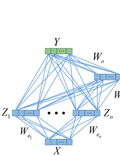
Figure 1: The architecture of a BLS [5]. Diverse linear de-noised features $\mathbf{Z}$ are extracted from data $\mathbf{X}$, and further mapped into nonlinear features $\mathbf{H}$. Linear features $\mathbf{Z}$ and nonlinear features $\mathbf{H}$ are then concatenated to predict $\mathbf{Y}$.

The steps to build a BLS are:

1. Construct the linear feature nodes $\mathbf{Z}$. Let $n$ be the number of groups of features nodes, and $m$ be the number of features nodes in each group. We first concatenate $\mathbf{X}$ with an all-one bias vector $\mathbf{1}\in\mathbb{R}^{N\times 1}$ to form the augmented data matrix $\mathbf{X}^{\prime}=[\mathbf{X}\ \mathbf{1}]$, then construct each of the $n$ groups of feature nodes, $\{\mathbf{Z}_{i}\}_{i=1}^{n}$, individually. For the $i$th group of feature nodes $\mathbf{Z}_{i}$, we first randomly generate uniformly distributed feature weights $\mathbf{W}_{r}\in\mathbb{R}^{(M+1)\times m}$ and compute the random feature nodes $\mathbf{Z}_{r_{i}}=\mathbf{X}^{\prime}\mathbf{W}_{r}$, then use least absolute shrinkage and selection operator (LASSO) to obtain sparse weights $\mathbf{W}_{e_{i}}\in\mathbb{R}^{(M+1)\times m}$:

   $$\mathbf{W}_{e_{i}} =\arg\min_{\mathbf{W}}(\frac{1}{2}||\mathbf{Z}_{r_{i}}\mathbf{W}-\mathbf{X}^{\prime}||_{F}^{2}+\lambda_{1}||\mathbf{W}||_{1,1})^{T},$$ (1)

   where $||\mathbf{W}||_{1,1}=\sum_{i=1}^{m}\sum_{j=1}^{M+1}\left|w_{ij}\right|$, and $\lambda_{1}$ is the L1 regularization coefficient. Alternating direction method of multipliers [8] is applied to solve (1). Then, we construct $\mathbf{Z}_{i}=\mathbf{X}^{\prime}\mathbf{W}_{e_{i}}$, and $\mathbf{Z}=[\mathbf{Z}_{1},...,\mathbf{Z}_{n}]$.

2. Construct the $k$ nonlinear enhancement nodes $\mathbf{H}$. Let $\xi$ be the hyperbolic tangent sigmoid function, i.e.,

   $$\xi(x)=\frac{2}{1+e^{-2x}}-1$$ (2)

   then

   $$\mathbf{H}^{\prime} =[\mathbf{Z},\mathbf{1}]\mathbf{W}_{h},$$ (3)

   $$\mathbf{H} =\xi\left(\frac{s\mathbf{H}^{\prime}}{\max(\operatorname{abs}(\mathbf{H}^{\prime}))}\right),$$ (4)

   where $\mathbf{W}_{h}\in\mathbb{R}^{(nm+1)\times k}$ is a matrix of the orthonormal bases of a randomly generated uniformly distributed weight matrix in $\mathbb{R}^{(nm+1)\times k}$, $s$ is a scalar normalization factor, and $\max(\operatorname{abs}(\mathbf{H}^{\prime}))$ is the maximum absolute value of all elements in $\mathbf{H}^{\prime}$. The goal of $\frac{s\mathbf{H}^{\prime}}{\max(\operatorname{abs}(\mathbf{H}^{\prime}))}$ is to constrain the input to $\xi$ to $[-s,s]$, i.e., it performs normalization.

3. Calculate $\mathbf{W}_{o}\in\mathbb{R}^{(nm+k)\times C}$, the weights from $[\mathbf{Z},\mathbf{H}]$ to $\mathbf{Y}$. Ridge regression is used to compute $\mathbf{W}_{o}$, i.e.,

   $$\mathbf{W}_{o} =\arg\min_{\mathbf{W}}(||[\mathbf{Z},\mathbf{H}]\mathbf{W}-\mathbf{Y}||_{F}^{2}+\lambda_{2}||\mathbf{W}||_{F}^{2})$$

   $$=(\lambda_{2}\mathbf{I}+[\mathbf{Z},\mathbf{H}]^{T}[\mathbf{Z},\mathbf{H}])^{-1}[\mathbf{Z},\mathbf{H}]^{T}\mathbf{Y},$$ (5)

   where $\lambda_{2}$ is the L2 regularization coefficient.

The pseudocode of BLS is given in Algorithm 1. Through $n$ random feature weight matrices $\mathbf{W}_{r}$ and L1 regularization, BLS extracts multiple sets of diverse linear de-noised features $\mathbf{Z}$ (which help increase its generalization ability). Then, orthogonal mapping and sigmoid functions are used to construct the enhancement nodes $\mathbf{H}$ to introduce more nonlinearity (which help increase its model fitting power). Finally, $\mathbf{Z}$ and $\mathbf{H}$ are concatenated as the features for predicting $\mathbf{Y}$.

Algorithm 1 The single-view BLS training algorithm [5].

0:  $\mathbf{X}\in\mathbb{R}^{N\times M}$, the training data matrix;         $\mathbf{Y}\in\mathbb{R}^{N\times C}$, the corresponding one-hot coding label matrix of $\mathbf{X}$;        $n$, the number of feature node groups;        $m$, the number of feature nodes in each group;        $k$, the number of enhancement nodes;        $s$, the normalization factor;        $\lambda_{1}$, the L1 regularization coefficient for determining $\mathbf{W}_{e_{i}}$;        $\lambda_{2}$, the L2 regularization coefficient for determining $\mathbf{W}_{o}$.

0:  BLS weight matrices $\mathbf{W}_{e_{i}}\in\mathbb{R}^{(M+1)\times m}$ ($i=1,...,n$), $\mathbf{W}_{h}\in\mathbb{R}^{(nm+1)\times k}$, and $\mathbf{W}_{o}\in\mathbb{R}^{(nm+k)\times C}$.

  Construct $\mathbf{X}^{\prime}=[\mathbf{X},\mathbf{1}]$

  for $i=1$ to $n$ do

     Initialize $\mathbf{W}_{r}$ randomly;

     Calculate $\mathbf{Z}_{r_{i}}=\mathbf{X}^{\prime}\mathbf{W}_{r}$;

     Calculate $\mathbf{W}_{e_{i}}$ using (1);

     Calculate feature nodes $\mathbf{Z}_{i}=\mathbf{X}^{\prime}\mathbf{W}_{e_{i}}$;

  end for

  Construct $\mathbf{Z}=[\mathbf{Z}_{1},...,\mathbf{Z}_{n}]$;

  Construct an orthonormal basis matrix $\mathbf{W}_{h}\in\mathbb{R}^{(nm+1)\times k}$ from a randomly generated matrix in $\mathbb{R}^{(nm+1)\times k}$;

  Calculate the enhancement nodes $\mathbf{H}$ using (3) and (4);

  Calculate $\mathbf{W}_{o}$ using (5).

II-B Multi-View Broad Learning System (MvBLS)

BLS has achieved comparable performance, with much less computational cost, with deep learning approaches on two single-view image datasets [5]. However, it is not optimized for multi-view data. This subsection extends single-view BLS to multi-view.

The architecture of the proposed MvBLS is shown in Fig. 2. Without loss of generality, we only consider two views. The extension to more than two views is straightforward. The general idea is to construct the linear de-noised feature nodes of each view separately, concatenate the feature nodes from all views to construct the nonlinear enhancement nodes, and finally fuse the feature nodes and enhancement nodes together for prediction. By separating the two views in the first layer of the MvBLS and optimizing $\mathbf{Z}^{A}$ and $\mathbf{Z}^{B}$ separately, we may obtain better features than optimizing $\mathbf{Z}=[\mathbf{Z}^{A}\ \mathbf{Z}^{B}]$ directly (as in the case that we concatenate $\mathbf{X}^{A}$ and $\mathbf{X}^{B}$ and feed them altogether into a single BLS), because $\mathbf{Z}$ may be too long to be optimized effectively.

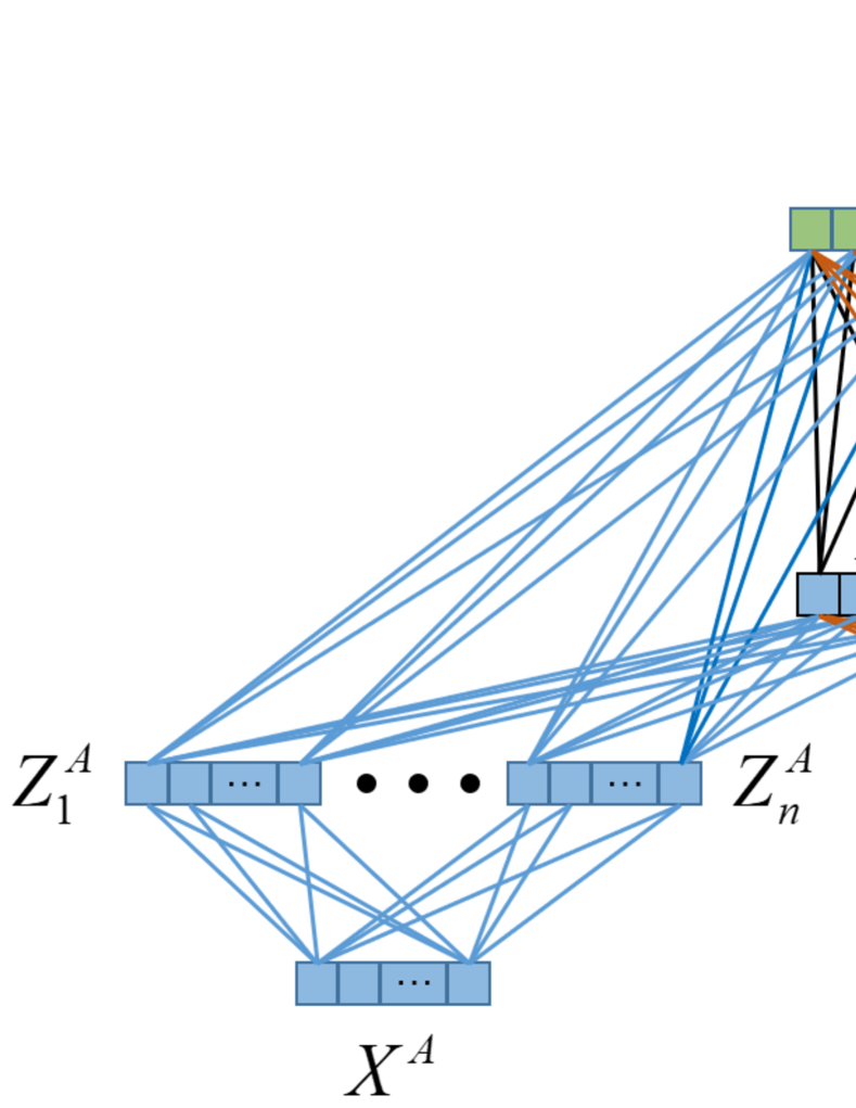
Figure 2: Architecture of the proposed MvBLS. Diverse linear de-noised features $\mathbf{Z}^{A}$ and $\mathbf{Z}^{B}$ are extracted from Views A and B, respectively. $\mathbf{Z}^{A}$ and $\mathbf{Z}^{B}$ are then mapped into nonlinear features $\mathbf{H}$. $\mathbf{Z}^{A}$, $\mathbf{Z}^{B}$ and $\mathbf{H}$ are next concatenated to predict $\mathbf{Y}$.

Let the two views be $A$ and $B$, the corresponding data matrices be $\mathbf{X}^{A}\in\mathbb{R}^{N\times M_{A}}$ and $\mathbf{X}^{B}\in\mathbb{R}^{N\times M_{B}}$ ($M_{A}$ and $M_{B}$ are the feature dimensionality of Views $A$ and $B$, respectively), and the shared label matrix be $\mathbf{Y}\in\mathbb{R}^{N\times C}$. The procedure for constructing the MvBLS is:

1. Construct the feature nodes $\mathbf{Z}^{A}=[\mathbf{Z}_{1}^{A},...,\mathbf{Z}_{n}^{A}]$ for View $A$, and $\mathbf{Z}^{B}=[\mathbf{Z}_{1}^{B},...,\mathbf{Z}_{n}^{B}]$ for View $B$, using Step (1) of Algorithm 1.

2. Construct the enhancement nodes $\mathbf{H}$, using the concatenated feature nodes $[\mathbf{Z}^{A},\mathbf{Z}^{B}]$ from both views and Step (2) of Algorithm 1.

3. Calculate $\mathbf{W}_{o}\in\mathbb{R}^{(2nm+k)\times C}$, the weights from $[\mathbf{Z}^{A},\mathbf{Z}^{B},\mathbf{H}]$ to $\mathbf{Y}$. Again, ridge regression is used to compute $\mathbf{W}_{o}$. Let $\mathbf{Z}^{\prime}=[\mathbf{Z}^{A},\mathbf{Z}^{B},\mathbf{H}]$. Then,

   $$\mathbf{W}_{o} =\arg\min_{\mathbf{W}}(||\mathbf{Z}^{\prime}\mathbf{W}-\mathbf{Y}||_{F}^{2}+\lambda_{2}||\mathbf{W}||_{F}^{2})$$

   $$=(\lambda_{2}\mathbf{I}+\mathbf{Z}^{\prime T}\mathbf{Z}^{\prime})^{-1}\mathbf{Z}^{\prime T}\mathbf{Y},$$ (6)

   where $\lambda_{2}$ is the L2 regularization coefficient.

The pseudocode for MvBLS is shown in Algorithm 2.

Algorithm 2 The proposed MvBLS for two views.

0:  $\mathbf{X}^{A}\in\mathbb{R}^{N\times M_{A}}$, the training data matrix for View $A$;         $\mathbf{X}^{B}\in\mathbb{R}^{N\times M_{B}}$, the training data matrix for View $B$;         $\mathbf{Y}\in\mathbb{R}^{N\times C}$, the corresponding one-hot coding label matrix;        $n$, the number of feature node groups;        $m$, the number of feature nodes in each group;        $k$, the number of enhancement nodes;        $s$, the normalization factor;        $\lambda_{1}$, the L1 regularization coefficient for determining $\mathbf{W}_{e_{i}}$;        $\lambda_{2}$, the L2 regularization coefficient for determining $\mathbf{W}_{o}$.

0:  MvBLS weight matrices $\mathbf{W}_{e_{i}}^{A}\in\mathbb{R}^{(M_{A}+1)\times m}$, $\mathbf{W}_{e_{i}}^{B}\in\mathbb{R}^{(M_{B}+1)\times m}$ ($i=1,...,n$), $\mathbf{W}_{h}\in\mathbb{R}^{(2nm+1)\times k}$, and $\mathbf{W}_{o}\in\mathbb{R}^{(2nm+k)\times C}$

  Calculate $\mathbf{W}_{e_{i}}^{A}$ and $\mathbf{W}_{e_{i}}^{B}$ using $\mathbf{X}^{A}$, $\mathbf{X}^{B}$, $\mathbf{Y}$, and Step (1) of BLS to construct the feature nodes $\mathbf{Z}^{A}$ and $\mathbf{Z}^{B}$;

  Calculate $\mathbf{W}_{h}$ using $\mathbf{Z}^{A}$, $\mathbf{Z}^{B}$, and Step (2) of BLS;

  Calculate $\mathbf{W}_{o}$ using (6).

III Experiment and Results

This section applies BLS and MvBLS to monkey oculomotor decision classification, and compares their performance with those using several classical and state-of-the-art single-view and multi-view learning approaches.

III-A The Neurophysiology Experiment

The invasive neurophysiological experimental setup used here and animal behavior were reported in [9]. All animal care and experimental procedures were in compliance with the US Public Health Service policy on the humane care and use of laboratory animals, and were approved by Johns Hopkins University Animal Care and Use Committee.

Two male rhesus monkeys (Monkey A: 7.5 kg; Monkey I: 7.2 kg) were trained to perform an oculomotor gambling task, as shown in Fig. 3. In each trial, the monkeys chose between two gamble options by making an eye movement (saccade) towards one of the visual cues. Two visual cues were randomly presented in two of four fixed locations (top right, bottom right, top left, and bottom left). Each cue was comprised of two colors (from a four-color library of cyan, red, blue, and green) and each color was associated with an amount of reward (1, 3, 5 to 9 units of water respectively, where 1 unit equaled 30 $\mu$L). The background color of a visual cue was cyan (small reward), and the foreground color was either red, or blue, or green (larger reward). The proportion of the two colors represented the probability of winning the corresponding reward. For the red/cyan target in Fig. 3, there was a 60% probability of having one unit of water (cyan color), and a 40% probability of having three units of water (red color). The expected reward value would then be $0.6\times 1+0.4\times 3=1.8$ units of water. There were a total of seven gamble options, representing three different expected reward values, as shown in Fig. 4.

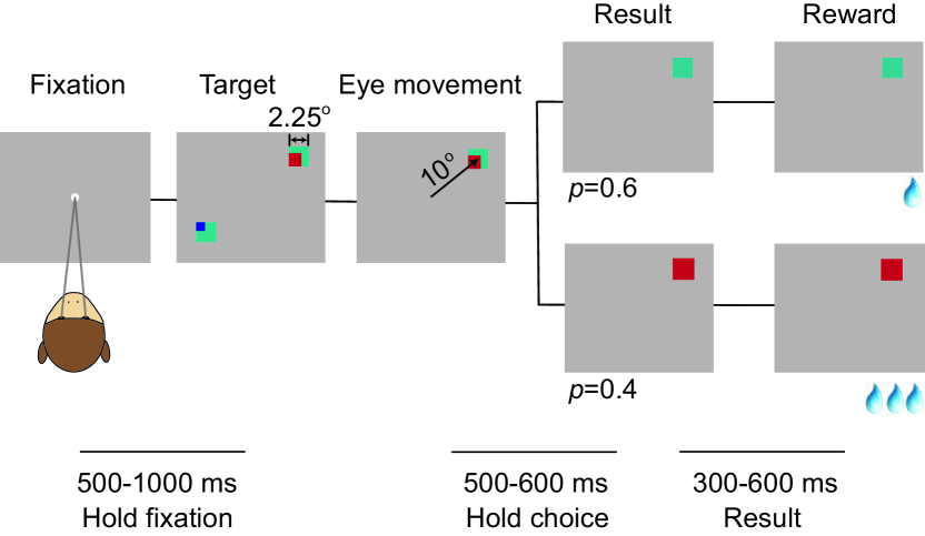
Figure 3: Sequence of events in the oculomotor gambling task. The figure is modified from Figure 2B in [9]. In the ‘target’ step, two visual cues appeared in two random directions. After the visual cues were presented, the monkey made a choice between the two options by making a saccade to the corresponding visual cue (‘saccade’ step), indicted by the black arrow (the black arrow was artificially added to the figure to better explain the experiment design, but it was not included in the actual visual cue displayed to the monkeys). The lines at the bottom indicate the duration of various time periods in the gambling task.

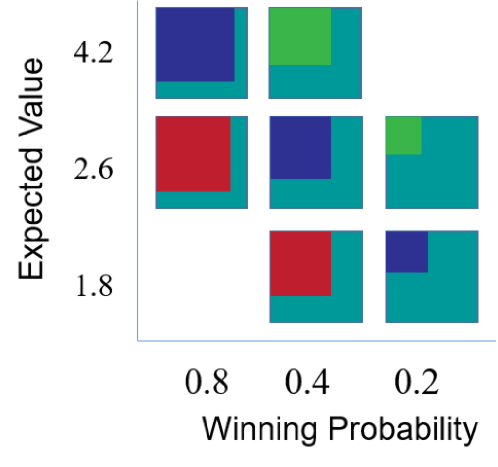
Figure 4: The seven visual cues used in the gambling task. The figure is modified from Figure 2A in [9]. Four different colors (cyan, red, blue, and green) indicated different amounts of reward (increasing from 1, 3, 5 to 9 units of water, where 1 unit equaled 30 $\mu$L). For example, the expected value of the right green/cyan target is: 9 units (reward amount) $\times$ 0.2 (reward probability) $+$ 1 unit (reward amount) $\times$ 0.8 (reward probability) $=$ 2.6 units.

Neural signals from the monkeys’ supplementary eye field in the medial frontal cortex were recorded with one or more tungsten electrodes, and the monkeys’ corresponding choices were recorded using an eye tracking system (Eye Link, SR Research Ltd, Ottawa, Canada).

The goal of our study was to investigate the task of decoding eye movements (choice intention) from neural signals in the primate medial frontal cortex, which are causally involved in risky decisions [10].

III-B Datasets

Forty-five datasets [9] were recorded from 45 experiment sessions from the two monkeys (33 from Monkey A, and 12 from Monkey I). Their statistics are shown in Table I, where $d_{1}$-$d_{4}$ denote the four different saccade directions (classes), $nE$ the number of electrodes in recording the LFPs, and $nU$ the number of units in recording the spikes.

For each recording, electrodes were lowered into the monkeys’ supplementary eye field using electric microdrives. While the monkeys were preforming the task, activity was recorded extracellularly using 1 to 4 tungsten microelectrodes with an impedance of 2-4 M$\Omega$s (Frederick Haer, Bowdoinham, ME, USA) spaced 1-3 mm apart. Neural activity was measured against a local reference, a stainless steel guide tube, which carried the electrode array and was positioned above the dura.

At the preamplifier stage, signals were processed with 0.5 Hz 1-pole high-pass and 8k Hz 4-pole low-pass anti-aliasing Bessel filters, and then divided into two streams for the recording of LFPs and spiking activity. The stream used for LFP recording was amplified (500-2000 gain), processed by a 4-pole 200 Hz low-pass Bessel filter, and sampled at 1000 Hz. The stream used for spike detection was processed by a 4-pole Bessel high-pass filter (300 Hz), a 2-pole Bessel low-passed filter (6000 Hz), and was sampled at 40k Hz. Up to four template spikes were identified using principal component analysis. The spiking activity was subsequently analyzed off-line. To maximize task related information in the spiking activity, all spike waveforms above the sorting threshold were used in the analysis. They included spiking activities from single units, multi-units, unsorted units, and units with very low firing rates.

Fig. 5 illustrates two single units, two multi-units and an unsorted units we identified in a representative recording. A single-unit is defined as a well-isolated unit (see Fig. 5(b)) whose interspike interval (ISI) violation rate (see Fig. 5(c)) is smaller than 0.02. A multi-unit is defined as a unit with a clear template waveform (online or offline); however, it is not well isolated from other clusters of waveforms (see Fig. 5(b)) and has a high ISI violation rate ($\geq 0.02$). An unsorted unit is defined by the Plexon Offline Sorter, whose spike waveforms do not belong to any category of sorted waveforms (see Figs. 5(b) and (e)) [11, 12, 13]. Finally, spikes were counted within each millisecond bin. Therefore, the temporal frequency of the spiking activity was 1000 Hz.

In the remainder of the paper, we refer both multi-units and unsorted units as multi-units for simplicity.

Figure 5: A representative recording (a-d) and population spike waveforms from all experimental sessions. (a) Average spike waveforms for unsorted unit, multi-units, and single-units recorded from the same electrode; (b) scatter plot of spike waveforms using the first two principal components; (c) ISI histogram of a single unit (bin width 1 ms); (d) cross-correlograms between two single-units; and (e) average spike waveforms of all recorded units (unsorted units are in grey).

TABLE I: Statistics of the 45 datasets.

Dataset	Number of trials						$nE$	$nU$	$nS$	$nM$
	$d_{1}$	$d_{2}$	$d_{3}$	$d_{4}$	Avg	Std
1	218	236	169	142	191	43.35	4	20	5	15
2	255	259	195	189	225	37.64	3	16	5	11
3	275	310	256	195	259	48.17	3	14	5	8
4	198	187	197	141	181	26.96	3	13	7	6
5	203	210	146	153	178	33.16	3	13	6	7
6	218	231	213	190	213	17.11	3	15	10	5
7	159	184	161	142	162	17.25	3	16	10	6
8	170	193	188	164	179	13.94	3	14	9	5
9	194	183	197	177	188	9.36	3	11	4	7
10	222	249	220	195	222	22.07	3	16	7	9
11	224	235	242	212	228	13.12	3	14	7	7
12	121	114	140	129	126	11.17	2	10	4	6
13	193	177	178	189	184	7.97	3	14	5	9
14	251	220	201	192	216	26.09	2	10	2	8
15	227	211	184	176	200	23.67	2	7	1	6
16	207	188	183	156	184	21.05	2	8	2	6
17	225	203	131	173	183	40.69	2	8	0	8
18	228	208	194	188	205	17.77	2	10	1	9
19	185	166	149	148	162	17.42	3	13	3	10
20	169	147	145	164	156	12.04	1	3	1	2
21	170	151	117	137	144	22.38	1	4	1	3
22	163	144	102	126	134	26.00	1	5	1	4
23	193	192	171	182	185	10.28	1	4	3	1
24	196	183	164	172	179	13.89	1	3	1	2
25	148	138	104	138	132	19.25	2	7	3	4
26	209	166	129	182	172	33.43	2	9	5	4
27	218	168	133	210	182	39.48	2	9	1	8
28	183	161	118	164	157	27.45	1	2	0	2
29	198	173	111	170	163	36.87	3	13	8	5
30	188	181	144	143	164	23.85	3	12	4	8
31	216	189	174	212	198	19.81	3	14	6	8
32	213	206	137	213	192	36.98	3	14	9	5
33	198	174	116	179	167	35.38	3	13	5	7
34	212	188	115	178	173	41.37	3	14	7	7
35	304	274	168	274	255	59.70	3	14	3	11
36	274	222	134	245	219	60.37	3	14	7	7
37	263	202	114	204	196	61.41	3	14	5	9
38	244	202	160	202	202	34.29	3	13	2	11
39	249	240	134	223	212	52.78	3	15	8	7
40	273	253	182	220	232	39.86	3	15	7	8
41	133	136	134	123	132	5.80	2	9	6	3
42	138	154	141	117	138	15.33	3	11	3	8
43	283	248	232	246	252	21.70	3	15	8	7
44	194	187	129	162	168	29.41	3	15	8	7
45	146	187	145	124	151	26.36	3	15	8	7
Avg	208	196	160	177	185	27.85	$-$	$-$	$-$	$-$

III-C LFP and Spike Feature Extraction

In this study, single-unit and multi-unit spikes were smoothed through 100-point moving average. The LFPs and processed spikes were then epoched to $[0,400)$ ms with 1 ms temporal resolution after target onset for each electrode/unit. The eye movement reaction times (the time between target onset and eye movement onset) for the monkeys ranged from 100 ms to 300 ms. Therefore, the monkeys finished their eye movement before the end of each trial.

Each trial had two views: the spike view and the LFP view. The spike view had $400\cdot nU$ features, where $nU$ is the number of units for spikes in Table I. For each LFP trial from each electrode, power spectrum density of the 400-ms signal was computed by the Welch’s method with a Hamming window of 88 ms and 50% overlap. Then, log-power in eight frequency bands (theta, 4-8 Hz; alpha, 8-12 Hz; beta 1, 12-24 Hz; beta 2, 24-34 Hz; gamma 1, 34-55 Hz; gamma 2, 65-95 Hz; gamma 3, 130-170 Hz; gamma 4, 170-200 Hz), as used in [14], were calculated and concatenated with the 400-ms signal as the features. Therefore, the LFP view had $408\cdot nE$ features, where $nE$ is the number of electrodes for LFPs in Table I. Finally, both spike and LFP features were $z$-normalized.

III-D Algorithms

We compared the performance of different decoding algorithms, including both single-view learning and multi-view learning approaches:

1. Support vector machine (SVM), which uses error-correcting output codes (ECOC) [15] for multi-class classification. SVM is a classical statistical machine learning approach, and has achieved outstanding performance in numerous applications. The box constraint $C$ was chosen from $\{10^{-6},10^{-4},\cdots,10^{6}\}$ by nested cross-validation. Each binary SVM classifier was solved by sequential minimal optimization (SMO) [16], and the optimization stopped if the gradient difference between upper and lower violators obtained by SMO was smaller than $0.001$.

2. Ridge classification (Ridge), which performs ridge regression to approximate the $\{0,1\}$ output of each class, and then classifies the input to the class with the largest output. The L2 regularization coefficient $\lambda_{2}$ was chosen from $\{10^{-6},10^{-4},\cdots,10^{6}\}$ by nested cross-validation.

3. BLS, which has been introduced in Section II-A. We used normalization factor $s=0.8$ and L1 regularization coefficient $\lambda_{1}=0.001$, and selected the number of feature node groups $n$ from $\{10,20\}$, the number of feature nodes in each group $m$ from $\{10,20\}$, the number of enhancement nodes $k$ from $\{100,500\}$, and the L2 regularization coefficient $\lambda_{2}$ from $\{10^{-6},10^{-4},\cdots,10^{6}\}$, using nested cross-validation. The alternating direction method of multipliers [8] used to solve (1) for feature nodes construction was iterative, and it terminated after 50 iterations.

4. Multi-view discriminant analysis with view-consistency (MvDA) [17], which extends classical single-view linear discriminant analysis to multi-view learning, and adds a regularization term to enhance the view-consistency.

5. Multi-view modular discriminant analysis (MvMDA) [18], which exploits the distance between class centers across different views.

6. MvBLS, which has been introduced in Section II-B. Its parameter tuning was the same as that for BLS.

Note that the first three algorithms can be used for both single-view learning and multi-view learning. When they were used in multi-view learning, we simply combined the features from different views as a single view input to the classifier. The last three approaches were used in multi-view learning only. The subspace dimensionality of MvDA and MvMDA was set to three (the number of classes minus one). After subspace alignment, the subspace features of all views were concatenated and fed into an ECOC-SVM classifier, where the same nested cross-validation was conducted as in the SVM approach. Linear kernel was employed in all SVMs.

We randomly partitioned each dataset into three subsets: 60% for training, 20% for validation, and the remaining 20% for test. We repeated this process 30 times on each of the 45 datasets, and recorded the test classification accuracies as our performance measure.

III-E 4-Class Classification Using only the LFPs

In the first experiment, we used only the LFPs in 4-class classification. The classification accuracies in the 45 sessions, each averaged over 30 cross-validation runs, are shown in the bar graph in the top panel of Fig. 6, and also in the box plot in the top-left panel of Fig. 7. The last group of the bar plot also shows the average accuracies across the 45 sessions, whose numerical values are given in Table II. Each standard deviation showed in Table II was computed from 30 average accuracies of the 45 sessions. On average BLS slightly outperformed SVM and Ridge, which was also true in 29 and 32 out of the 45 individual sessions, respectively.

To find out whether there were statistically significant differences between different algorithms, non-parametric multiple pairwise comparison tests using Dunn’s procedure [19], with a $p$-value correction using the False Discovery Rate method [20], were performed on the cross-validation accuracies. The null hypothesis in each pairwise comparison was the probability of observing a randomly selected value from the first group that is larger than a randomly selected value from the second group equals $0.5$, and it was rejected if $p\geq\alpha/2$, where $\alpha=0.05$. The $p$-values, when only the LFP features were used, are shown in the first part of Table III. There was no statistically significant difference between any pair of algorithms.

In summary, we have shown that when only the LFP features were used, SVM, Ridge and BLS achieved comparable classification performances (BLS may be slightly better, but there was no statistically significant difference).

III-F 4-Class Classification Using only the Spikes

In the second experiment, we used only the spikes in 4-class classification. The classification accuracies in the 45 sessions, each averaged over 30 cross-validation runs, are shown in the bar graph in the middle panel of Fig. 6, and also in the box plot in the top-right panel of Fig. 7. The last group of the bar graph shows the average accuracies across the 45 sessions, whose numerical values are also given in Table II. For all algorithms, using spikes only achieved better classification accuracy than using LFPs only. On average Ridge slightly outperformed BLS, which was also true in 32 individual sessions. Interestingly, the opposite held when the LFP features were used. This may indicate that LFPs and spikes encode non-identical information about the oculomotor decision.

Non-parametric multiple comparison tests were also performed, and the $p$-values are shown in the second part of Table III. There was no statistically significant difference between any pair of algorithms.

In summary, we have shown that when only the spike features were used, SVM, Ridge and BLS again achieved comparable classification performance (Ridge may be slightly better, but there was no statistically significant difference).

III-G 4-Class Classification Using both LFPs and Spikes

In the third experiment, we used both LFPs and spikes in 4-class classification. The classification accuracies of MvBLS in the 45 sessions, each averaged over 30 cross-validation runs, are shown in horizontal-axis of three scatter plots in the bottom panel of Fig. 6, and also the box plot in the bottom panel of Fig. 7. The average accuracies across the 45 sessions are given in Table II. Observe that:

1. The proposed MvBLS using LFPs+Spikes outperformed BLS using LFPs significantly, which is the best-performing approach using LFPs.

2. The proposed MvBLS using LFPs+Spikes outperformed Ridge using Spikes significantly, which is the best-performing approach using Spikes.

3. On average, the two subspace multi-view learning algorithms, i.e., MvDA and MvMDA, performed much worse than the three single-view algorithms, i.e., SVM, Ridge, and BLS.

4. On average, our proposed MvBLS outperformed the two subspace multi-view learning algorithms. This suggests that MvBLS can extract more discriminative features and better fuse them than the other two approaches.

5. On average, our proposed MvBLS also outperformed the three single-view learning algorithms. This suggests that fusing the two views in a more sophisticated way may be more advantageous than simply concatenating and feeding them into a single-view classifier.

Non-parametric multiple comparison tests were also performed, and the $p$-values are shown in Table IV, where the statistically significant ones are marked in bold. There was statistically significant difference between MvBLS and each of the other five algorithms.

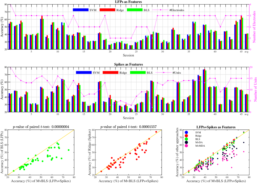
Figure 6: 4-class classification accuracies of different algorithms, when different features were used.

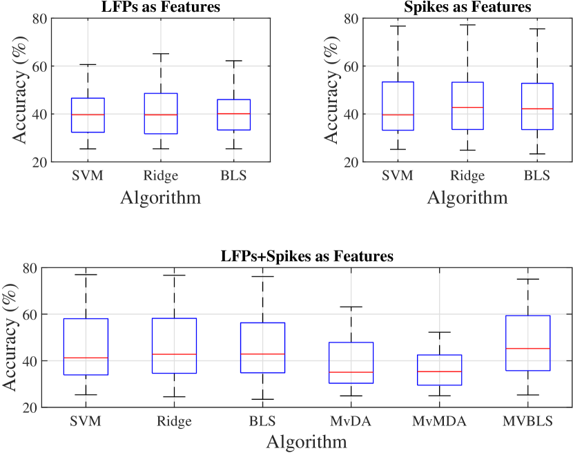
Figure 7: Boxplots of the 4-class classification accuracies of different algorithms, using different features. The red line in the box indicates the median, and the bottom and top edges of the box indicate the 25th and 75th percentiles, respectively. The whiskers extend to the most extreme data points, excluding outliers.

TABLE II: Mean and standard deviation of 4-class classification accuracies (%) when different classifiers and features were used.

	SVM	Ridge	BLS	MvDA	MvMDA	MvBLS
LFPs	40.57$\pm$0.70	40.85$\pm$0.70	41.24$\pm$0.62	$-$	$-$	$-$
Spikes	43.49$\pm$0.62	44.21$\pm$0.47	43.48$\pm$0.59	$-$	$-$	$-$
LFPs+Spikes	46.12$\pm$0.56	46.51$\pm$0.41	45.65$\pm$0.52	39.49$\pm$0.50	36.62$\pm$0.55	47.94$\pm$0.62

TABLE III: $p$-values of non-parametric multiple comparisons, when only the LFP features (first part) and the spike features (second part) were used in 4-class classification.

	LFP Features		Spikes Features
	SVM	Ridge	SVM	Ridge
Ridge	.4148		.1224
BLS	.2607	.1892	.3827	.1118

TABLE IV: $p$-values of non-parametric multiple comparisons, when both LFPs and spikes were used in 4-class classification.

	SVM	Ridge	BLS	MvDA	MvMDA
Ridge	.2054
BLS	.2652	.0772
MvDA	.0000	.0000	.0000
MvMDA	.0000	.0000	.0000	.0000
MvBLS	.0001	.0019	.0000	.0000	.0000

We also compared MvBLS with random guess in 4-class classification. The results are shown in Fig. 8. Note that the random guess approach obtained slightly different accuracies in different sessions (not always exactly 25% in 4-class classification), because different classes had different numbers of trials. On average the 4-class classification accuracy of MvBLS was about twice of that of random guess (47.94% vs 25.04%), suggesting that a sophisticated machine learning approach like MvBLS can indeed mine useful information from LFPs and spikes.

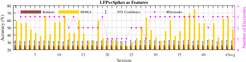
Figure 8: 4-class classification accuracies of permutation tests [9] with 95% confidence and MvBLS.

Finally, to validate if LFPs and spikes do contain complementary information in from another perspective, we counted the number of sessions that LFPs+Spikes achieved better performance than LFPs or spikes only, and show the results in Table V. Regardless of which classifier was used, LFPs+Spikes always outperformed LFPs or Spikes alone, in most sessions. Moreover, when MvBLS was used, LFPs+Spikes outperformed the best LFPs performance (among SVM, Ridge and BLS) in 40 sessions (88.89%), and the best Spikes performance in 32 sessions (71.11%).

TABLE V: Number and percentage of sessions (among the 45 sessions) that LFPs+Spikes outperformed a single modality of feature alone.

	Number of sessions LFP+Spikes outperformed
	LFPs	Spikes
SVM	31 (68.89%)	40 (88.89%)
Ridge	37 (82.22%)	28 (62.22%)
BLS	31 (68.89%)	35 (77.78%)

In summary, we have shown that LFPs and spikes contain complementary information about the brain’s oculomotor decision, and our proposed MvBLS can better fuse these features than several classical and state-of-the-art single-view and multi-view learning approaches.

IV Discussions

This section presents some additional discussions on the proposed MvBLS.

IV-A 4-Class Classification Accuracy versus the Number of Electrodes/Units

Figs. 6 and 8 show that sometimes the 4-class classification accuracy was very low, e.g., close to random guess (25.91%) or permutation tests [9] with 95% confidence (31.93%). The main reason is that the number of electrodes/units was small in these cases. For example, the top panel of Fig. 6 also shows the number of LFP electrodes in different sessions. It has a strong correlation with the classification accuracy, regardless of which classification algorithm was used. Particularly, the sessions with the lowest classification accuracy (Sessions 20-24) had the smallest number of electrodes. The middle panel of Fig. 6 shows the number of units in different sessions. Similar patterns can be observed.

Next, we performed a deeper investigation on how the number of electrodes in LFPs and the number of units in spikes affected the performance of BLS.

The LFPs were studied first. We identified all datasets with three or more electrodes, and considered each one separately. A dataset with three electrodes is used as an example to illustrate our experimental procedure. In the experiment, we randomly partitioned the dataset into 60% training, 20% validation, and 20% test. Then, we increased the number of chosen electrodes $k$ from one to two and then to three; for each $k$, we used LFPs from the corresponding electrodes to trained a BLS and compute its test accuracy. All possible combinations of $k$ electrodes were considered, and the average test accuracy was computed. After that, we repeated the data partition 30 times and computed the grand average test accuracies, as shown in Fig. 9. Intuitively, the classification accuracy increased with the number of electrodes. We would expect that higher classification accuracy could be obtained with more electrodes.

We next studied the decoding performance with spikes. The results are shown in Fig. 9. The experimental procedure was very similar to that for the LFPs, except one difference: the number of units associated with different electrodes were generally different, so the total number of units from $k$ electrodes could have different values. Take the first dataset with four electrodes (they had 4, 5, 5 and 6 units, respectively) as an example. All possible combinations of the 4 electrodes were considered. There were $C_{4}^{1}+C_{4}^{2}+C_{4}^{3}+C_{4}^{4}=15$ combinations, represented by the 15 blue circles in Fig. 9. We then connected these circles in the inclusive order, i.e., if two points $A$ and $B$ are on the same curve and $A$ is on the left of $B$, then the electrodes used to obtain $A$ were contained in the electrodes used to obtain $B$ (e.g., $A$ may be obtained from Electrodes 1 and 2, and $B$ from Electrodes 1, 2 and 3, or $B$ from Electrodes 1, 2, and 4). As a result, unlike in Fig. 9, where each dataset has only one curve, in Fig. 9 each dataset may have multiple branches leading to the same end-point. To make the curves more distinguishable, we only show the results for 10 datasets in Fig. 9. In general, the classification accuracy increased with the number of units, which is intuitive.

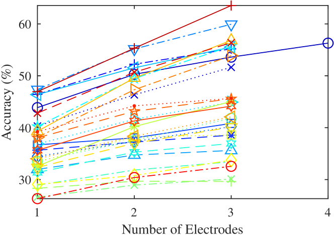
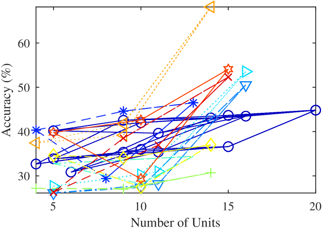
Figure 9: BLS classification (4-class) accuracy versus (a) the number of electrodes, and (b) the number of units. In (a), each curve represents a different dataset. In (b), curves with the same end-point are from the same dataset.

IV-B 4-Class Classification Using Single-Unit and Multi-Unit Spikes

We calculated the violation rate of the inter spike interval (ISI), which equalled the proportion of ISI shorter than three milliseconds. We defined a single-unit as a well isolated unit when the ISI violation rate is less than 0.02 [21]. The statistics are shown in Table I ($nU$ denotes the number of units, $nS$ the number of single units, and $nM$ the number of multi-units. Generally, $nU=nS+nM$, except in the third and 33rd datasets where one unit had almost no spikes and hence was removed).

We studied the 4-class classification performance with single-unit (denoted as sSpikes) and multi-unit (denoted as mSpikes) and combined units (single-unit + multi-unit, denoted as Spikes), respectively. For each condition, we performed single-view and multi-view 4-class classification on the 45 datasets for 30 times. The mean and standard deviation of the test classification accuracies are shown in Table VI. Observe that:

1. For classification using LFPs only, the features did not change, but the accuracies changed very slightly between three cases. This is because that the partition of training, validation and test sets were different in these three cases.

2. For classification using only spikes, Spikes had better performance than sSpikes and mSpikes. This indicates that Spikes contain more information than sSpikes and mSpikes, which is intuitive.

3. For classification using both LFPs and spikes, LFPs + Spikes had better performance than LFPs+sSpikes and LFPs+mSpikes. This again indicates that Spikes contain more information than sSpikes and mSpikes.

4. Combining LFP and spike features always improved the decoding performance.

5. Our proposed MvBLS achieved the best decoding performance in all conditions.

TABLE VI: Mean and standard deviation of 4-class classification accuracies (%) when different classifiers and features were used.

	SVM	Ridge	BLS	MvDA	MvMDA	MvBLS
LFPs	40.57$\pm$0.70	40.85$\pm$0.70	41.24$\pm$0.62	$-$	$-$	$-$
Spikes	43.49$\pm$0.62	44.21$\pm$0.47	43.48$\pm$0.59	$-$	$-$	$-$
LFPs+Spikes	46.12$\pm$0.56	46.51$\pm$0.41	45.65$\pm$0.52	39.49$\pm$0.50	36.62$\pm$0.55	47.94$\pm$0.62
LFPs	40.61$\pm$0.60	40.72$\pm$0.62	41.10$\pm$0.58	$-$	$-$	$-$
sSpikes	34.73$\pm$0.52	35.93$\pm$0.50	35.26$\pm$0.53	$-$	$-$	$-$
LFPs+sSpikes	41.46$\pm$0.62	41.54$\pm$0.63	41.20$\pm$0.58	36.41$\pm$0.63	32.92$\pm$0.79	43.37$\pm$0.77
LFPs	40.41$\pm$0.61	40.66$\pm$0.51	40.96$\pm$0.47	$-$	$-$	$-$
mSpikes	39.35$\pm$0.58	40.06$\pm$0.62	39.77$\pm$0.59	$-$	$-$	$-$
LFPs+mSpikes	43.92$\pm$0.47	44.04$\pm$0.64	43.36$\pm$0.51	38.64$\pm$0.58	35.05$\pm$0.69	45.16$\pm$0.57

IV-C Binary Classification Using Single-Unit and Multi-Unit Spikes

Four-class classification was considered in previous subsections, where we decoded one location out of all four possibilities. This subsection considers binary classification, where we decode one location out of the two available choices. Specifically, based on the classification confidences of the four possible locations, we calculated the binary test accuracies given the two locations available for choice. We performed single-view and multi-view classification on the 45 datasets for 30 times. The mean and standard deviation of binary test classification accuracies are shown in Table VII.

TABLE VII: Mean and standard deviation of binary classification accuracies (%) when different classifiers and features were used.

	SVM	Ridge	BLS	MvDA	MvMDA	MvBLS
LFPs	63.49$\pm$0.51	62.52$\pm$0.58	63.55$\pm$0.52	$-$	$-$	$-$
Spikes	67.47$\pm$0.63	67.14$\pm$0.66	67.25$\pm$0.67	$-$	$-$	$-$
LFPs+Spikes	69.13$\pm$0.56	68.45$\pm$0.60	68.24$\pm$0.53	62.67$\pm$0.66	60.84$\pm$0.63	69.51$\pm$0.56
LFPs	63.89$\pm$0.59	62.67$\pm$0.63	63.71$\pm$0.62	$-$	$-$	$-$
sSpikes	60.32$\pm$0.73	60.15$\pm$0.73	60.39$\pm$0.72	$-$	$-$	$-$
LFPs+sSpikes	64.83$\pm$0.68	63.92$\pm$0.58	64.16$\pm$0.56	60.27$\pm$0.68	57.57$\pm$0.66	65.71$\pm$0.59
LFPs	63.51$\pm$0.50	62.52$\pm$0.58	63.61$\pm$0.50	$-$	$-$	$-$
mSpikes	64.23$\pm$0.68	63.91$\pm$0.45	64.09$\pm$0.74	$-$	$-$	$-$
LFPs+mSpikes	67.28$\pm$0.53	66.39$\pm$0.54	66.28$\pm$0.55	62.05$\pm$0.60	59.35$\pm$0.59	67.58$\pm$0.53

The binary classification accuracies in Table VII are significantly above chance (50%). Intuitively, they are also much higher than their 4-class classification counterparts in Table VI. However, the observations made in the previous subsection still hold. Specifically, Spikes outperformed sSpikes and mSpikes, LFPs+Spikes outperformed LFPs+sSpikes and LFPs+mSpikes, combining LFP and spike features always improved the decoding performance, and our proposed MvBLS always achieved the best decoding performance.

IV-D MvBLS Parameter Sensitivity

MvBLS has three structural parameters and three nomalization/regularization parameters ($n$, $m$, $k$, $s$, $\lambda_{1}$ and $\lambda_{2}$ in Algorithm 2). It is important to know the sensitivity of MvBLS to them, which will provide valuable guidelines in selecting these parameters in future applications.

By default $n=15$, $m=15$, $k=300$, $s=0.8$, $\lambda_{1}=0.001$ and $\lambda_{2}=1$. When studying the sensitivity of MvBLS to $n$, we fixed $m$, $k$, $s$, $\lambda_{1}$ and $\lambda_{2}$ at their default values, and varied $n$ from $10$ to $100$. For each $n$ on each dataset, we trained 30 MvBLSs on 30 different partitions of the dataset (80% for training and 20% for test), and recorded the average test accuracy across the 30 runs. Finally we took the average of the 45 datasets, and show the results in the top-left panel of Fig. 10. Similarly, we varied $m$ from $10$ to $100$, $k$ from $50$ to $500$, $s$ from $0.25$ to $2.5$, $\lambda_{1}$ from $10^{-5}$ to $0.1$, and $\lambda_{2}$ from $0.01$ to $100$, and show the results in Fig. 10. Observe that:

1. As $n$ or $m$ increased, the training accuracy increased quickly, but the test accuracy slightly decreased. This suggests that smaller $n$ and $m$ should be used for better generalization performance, which is beneficial to the computational cost.

2. The training and test accuracies almost did not change with $k$ and $\lambda_{1}$. So, we can set $k$ to be a small value to save the computational cost, and choose $\lambda_{1}$ safely in $[0.00001,0.1]$.

3. As $s$ increased, the training accuracy increased slowly, but the test accuracy almost did not change. So, we can choose $s$ safely in $[0.25,2.5]$.

4. As $\lambda_{2}$ increased, the training accuracy decreased very quickly, but the test accuracy first increased slightly and then decreased slightly. This suggests that the regularization should not be too small or too large, which is a well-known fact in machine learning.

In general, we conclude that MvBLS is robust to its parameters.

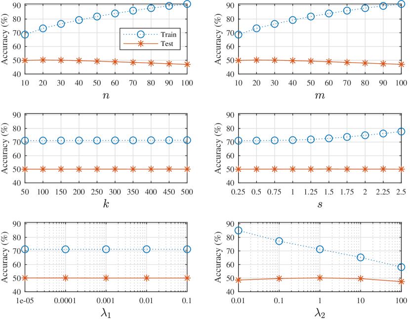
Figure 10: MvBLS classification (4-class) accuracy versus its parameters.

IV-E Computational Cost

Next, we compared the computational cost of different algorithms, as in practice a faster algorithm is preferred over a slower one, given similar classification accuracies.

We recorded the mean running time (including training, validation and test time) of 45 sessions for different classifiers, when different features were used. Since this process was repeated 30 times, we obtained 30 mean running time for each algorithm-feature combination. The mean and standard deviation for each combination were computed from these 30 numbers and shown in Table VIII. The platform was a Linux workstation with Intel Xeon CPU (E5-2699@2.20GHz) and 500GB RAM. SVM was the most efficient single-view learning algorithm, and MvBLS the most efficient multi-view learning algorithm. Particularly, MvBLS was several times faster than the other two state-of-the-art multi-view learning approaches, and it also achieved the best performance. In summary, our proposed MvBLS is both effective and efficient.

It is important to note that identifying the best model parameters in training is time-consuming, because a lot of cross-validations are needed; however, once the optimal model parameters are found, all models can be run very fast in test, which involves mostly matrix operations.

TABLE VIII: Mean and standard deviation of running time (seconds; including cross-validation to identify the best model parameters) when different classifiers and features were used in 4-class classification.

	SVM	Ridge	BLS	MvDA	MvMDA	MvBLS
LFPs	7.72$\pm$0.30	4.40$\pm$0.53	37.52$\pm$2.24	$-$	$-$	$-$
Spikes	19.05$\pm$2.92	585.54$\pm$52.87	85.77$\pm$5.42	$-$	$-$	$-$
LFPs+Spikes	24.84$\pm$3.19	1033.14$\pm$89.47	102.40$\pm$6.83	748.06$\pm$66.55	741.87$\pm$68.08	129.66$\pm$7.93

To better illustrate the above point, we removed the validation set and compared SVM and MvBLS when both LFPs and spikes were used as features. The box constraint of SVM was set to $10^{-4}$, which was the most frequently chosen value in Section III-G. The parameters of MvBLS were $n=15$, $m=15$, $k=300$, $s=0.8$, $\lambda_{1}=0.001$ and $\lambda_{2}=1$, which were the default values in Section IV-D. We also compared them with a multi-view deep learning approach, deep canonically correlated autoencoders (DCCAE) [22]. DCCAE aligned the two views of data in a common subspace and then used an ECOC-SVM classifier for classification. Its parameters were adjusted from the open source code by changing the mini-batch size for the correlation and the reconstruction error terms from 800 to 16, and the maximum number of epoches from 14 to 9, and the box constraint of SVM was set to $1$, as they gave higher classification accuracies. We ran the three models on each of the 45 sessions eight times. Each time we randomly partitioned the datasets into 80% training and 20% test. The platform was a laptop computer with AMD Ryzen 5 CPU (3550H@2.10GHz) and 16GB RAM, running Windows 10 x64 and Matlab 2020a. The mean and standard deviation of 4-class and binary classification accuracies on the test set, as well as the computing time (including both training and test on one dataset), are shown in Table IX. MvBLS achieved the highest classification accuracies, and was also the fastest.

TABLE IX: Mean and standard deviation of 4-class and binary classification accuracies, as well as the computing time, for different models, when both LFPs and Spikes were used as features.

	SVM	DCCAE	MvBLS
4-class accuracy (%)	46.77$\pm$0.05	39.20$\pm$0.07	50.35$\pm$0.08
Binary accuracy (%)	69.77$\pm$0.08	65.32$\pm$0.08	71.57$\pm$0.04
Computing time (s)	5.26$\pm$0.08	1409.20$\pm$1.31	1.99$\pm$0.04

IV-F Additional MvBLS Approaches

In addition to the MvBLS model in Fig. 2, other MvBLS architectures can also be configured, by constructing the inputs to $\mathbf{Y}$ differently. Two additional configurations are shown in Fig. 11, and denoted as MvBLS2 and MvBLS3, respectively. Compared with MvBLS in Fig. 2, MvBLS2 in Fig. 11 first constructs enhancement nodes $\mathbf{H}^{A}$ from $\mathbf{Z}^{A}$ and $\mathbf{H}^{B}$ from $\mathbf{Z}^{B}$, and then feeds all of them into $\mathbf{Y}$; so, it has more nodes and weights than MvBLS. Compared with MvBLS2, MvBLS3 in Fig. 11 further constructs enhancement nodes $\mathbf{H}$ from $\mathbf{Z}^{A}$ and $\mathbf{Z}^{B}$, and then feeds $\mathbf{H}$, $\mathbf{H}^{A}$, $\mathbf{H}^{B}$, $\mathbf{Z}^{A}$ and $\mathbf{Z}^{B}$ into $\mathbf{Y}$. So, MvBLS3 has even more nodes and weights than MvBLS2.

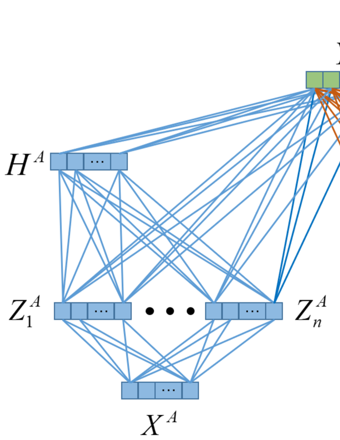
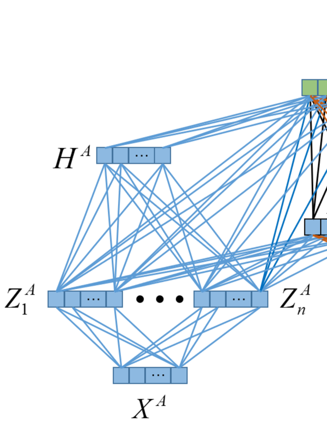
Figure 11: Two additional configurations of MvBLS. (a) MvBLS2; (b) MvBLS3.

The 4-class classification performances of MvBLS, MvBLS2 and MvBLS3 in the 45 sessions are shown in Fig. 12. Their classification accuracies were almost identical, which is interesting, considering that MvBLS2 and MvBLS3 had more parameters and connections. Indeed, non-parametric multiple comparisons showed that there was no statistically significant difference between any two of them. Since MvBLS has much simpler configuration and is easier to train, it is preferred in our application.

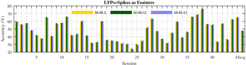
Figure 12: 4-class classification accuracies of the three different MvBLSs.

IV-G Related Work

Both LFPs and spikes contain information about the monkeys’ oculomotor decision, and there has been independent research on both. Spikes are high-pass filtered neural signals, which can be used to decode high-performance movement control signals [23, 24]. However, since spikes often deteriorate as electrodes degrade over time, more stable LFPs, which are low-pass filtered neural signals, are used in long term BMIs [25, 26, 27, 28, 29, 30].

Because LFPs and spikes can be recorded from the same electrodes [31], and convey complementary information [32, 33, 34, 35], a natural approach is to combine them for more accurate decoding [36, 37, 1, 38, 39, 14].

Bokil et al. [36] trained two macaque monkeys to perform a memory-saccade task and collected LFPs and spikes from the lateral intraparietal area. Two-dimensional Fourier transforms were performed to extract the features. Saccade prediction was achieved by maximizing the log-likelihood function of the observed neural activity. This approach was novel in that it did not use trial start time or other trial-related timing information. However, the performance degraded when switching from the preferred-or-anti-preferred binary classification to four-direction and eight-direction classifications.

Bansal et al. [39] trained two male macaque monkeys to perform reach-and-grasp tasks in three dimensions, and collected 192-channel LFPs and spikes from primary and ventral premotor areas. Linear Gaussian state-space representation and Kalman filter were then used to decode the reach-and-grasp kinematics. The decoding was first conducted for each channel, then about 30 channels were iteratively chosen based on the decoding performance (the Pearson correlation coefficient between the measured and the reconstructed kinematics). This approach required a large number of channels to be chosen from, which may not available in many human and non-human primate studies, including ours.

Hsieh et al. [14] trained one adult rhesus macaque to perform a center-out-and-back task and collected 137-channel LFPs and spikes from dorsal premotor cortex and ventral premotor cortex of both hemispheres. They then developed a multi-scale encoding model, a multi-scale adaptive learning algorithm, and a multi-scale filter for decoding the millisecond time-scale of spikes and slower LFPs. This approach solved a trajectory regression problem, whereas we focused on oculomotor decision classification.

Most studies, except [39] and [14] introduced above have not shown significant improvements in decoding performance, compared with using LFPs or spikes alone. Our research has shown that sophisticated machine learning approaches like MvBLS can better fuse LFPs and spikes, and hence achieve significant decoding performance improvements.

V Conclusion

Multi-view learning is beneficial for decoding oculomotor decisions using medial frontal neural signals from non-human primates. This is because these simultaneously recorded neural signals comprise both low-frequency LFPs and high-frequency spikes, which can be treated as two views of the brain state. In this paper, we have extended single-view BLS to MvBLS, and validated its performance in monkey oculomotor decision decoding from medial frontal LFPs and spikes. We demonstrated that primate medial frontal LFPs and spikes do contain complementary information about the oculomotor decisions, and that the proposed MvBLS is a more effective approach to use these two types of information in decoding the decision, than several classical and state-of-the-art single-view and multi-view learning approaches. Moreover, we showed that MvBLS is fast, and robust to its parameters. Therefore, we expect that MvBLS will find broader applications in other primate brain state decoding tasks, and beyond.

References

- [1] S. D. Stavisky, J. C. Kao, P. Nuyujukian, S. I. Ryu, and K. V. Shenoy, “A high performing brain-machine interface driven by low-frequency local field potentials alone and together with spikes,” Journal of Neural Engineering, vol. 12, no. 3, p. 036009, 2015.
- [2] M. Kandemir, A. Vetek, M. Gönen, A. Klami, and S. Kaski, “Multi-task and multi-view learning of user state,” Neurocomputing, vol. 139, pp. 97–106, 2014.
- [3] K. Pasupa and S. Szedmák, “Utilising Kronecker decomposition and tensor-based multi-view learning to predict where people are looking in images,” Neurocomputing, vol. 248, pp. 80–93, 2017.
- [4] L. Spyrou, S. Kouchaki, and S. Sanei, “Multiview classification and dimensionality reduction of scalp and intracranial EEG data through tensor factorisation,” Signal Processing Systems, vol. 90, no. 2, pp. 273–284, 2018.
- [5] C. P. Chen and Z. Liu, “Broad learning system: An effective and efficient incremental learning system without the need for deep architecture,” IEEE Trans. on Neural Networks and Learning Systems, vol. 29, no. 1, pp. 10–24, 2018.
- [6] M. Leshno, V. Y. Lin, A. Pinkus, and S. Schocken, “Multilayer feedforward networks with a nonpolynomial activation function can approximate any function,” Neural Networks, vol. 6, no. 6, pp. 861–867, 1993.
- [7] B. Igelnik and Y.-H. Pao, “Stochastic choice of basis functions in adaptive function approximation and the functional-link net,” IEEE Trans. on Neural Networks, vol. 6, no. 6, pp. 1320–1329, 1995.
- [8] S. Boyd, N. Parikh, E. Chu, B. Peleato, and J. Eckstein, “Distributed optimization and statistical learning via the alternating direction method of multipliers,” Foundations and Trends in Machine Learning, vol. 3, no. 1, pp. 1–122, 2010.
- [9] X. Chen and V. Stuphorn, “Sequential selection of economic good and action in medial frontal cortex of macaques during value-based decisions,” Elife, vol. 4, p. e09418, 2015.
- [10] X. Chen and V. Stuphorn, “Inactivation of medial frontal cortex changes risk preference,” Current Biology, vol. 28, no. 19, pp. 3114–3122.e4, 2018.
- [11] J. E. Chung, J. F. Magland, A. H. Barnett, V. M. Tolosa, A. C. Tooker, K. Y. Lee, K. G. Shah, S. H. Felix, L. M. Frank, and L. F. Greengard, “A fully automated approach to spike sorting,” Neuron, vol. 95, no. 6, pp. 1381–1394, 2017.
- [12] F. Kloosterman, S. P. Layton, Z. Chen, and M. A. Wilson, “Bayesian decoding using unsorted spikes in the rat hippocampus,” Journal of Neurophysiology, vol. 111, no. 1, pp. 217–227, 2014.
- [13] C. Trainito, C. von Nicolai, E. K. Miller, and M. Siegel, “Extracellular spike waveform dissociates four functionally distinct cell classes in primate cortex,” Current Biology, vol. 29, no. 18, pp. 2973–2982, 2019.
- [14] H.-L. Hsieh, Y. T. Wong, B. Pesaran, and M. M. Shanechi, “Multiscale modeling and decoding algorithms for spike-field activity,” Journal of Neural Engineering, vol. 16, no. 1, 2019.
- [15] T. G. Dietterich and G. Bakiri, “Solving multiclass learning problems via error-correcting output codes,” Journal of Artificial Intelligence Research, vol. 2, pp. 263–286, 1994.
- [16] R.-E. Fan, P.-H. Chen, and C.-J. Lin, “Working set selection using second order information for training support vector machines,” Journal of Machine Learning Research, vol. 6, no. Dec, pp. 1889–1918, 2005.
- [17] M. Kan, S. Shan, H. Zhang, S. Lao, and X. Chen, “Multi-view discriminant analysis,” IEEE Trans. on Pattern Analysis and Machine Intelligence, vol. 38, no. 1, pp. 188–194, 2016.
- [18] G. Cao, A. Iosifidis, K. Chen, and M. Gabbouj, “Generalized multi-view embedding for visual recognition and cross-modal retrieval,” IEEE Trans. on Cybernetics, vol. 48, no. 9, pp. 2542–2555, 2018.
- [19] O. Dunn, “Multiple comparisons using rank sums,” Technometrics, vol. 6, pp. 214–252, 1964.
- [20] Y. Benjamini and Y. Hochberg, “Controlling the false discovery rate: A practical and powerful approach to multiple testing,” Journal of the Royal Statistical Society, Series B (Methodological), vol. 57, pp. 289–300, 1995.
- [21] D. N. Hill, S. B. Mehta, and D. Kleinfeld, “Quality metrics to accompany spike sorting of extracellular signals,” Journal of Neuroscience, vol. 31, no. 24, pp. 8699–8705, 2011.
- [22] W. Wang, R. Arora, K. Livescu, and J. A. Bilmes, “On deep multi-view representation learning,” in Proc. 32nd Int’l Conf. on Machine Learning, Lille, France, July 2015, pp. 1083–1092.
- [23] D. R. Humphrey, E. Schmidt, and W. Thompson, “Predicting measures of motor performance from multiple cortical spike trains,” Science, vol. 170, no. 3959, pp. 758–762, 1970.
- [24] G. Santhanam, S. I. Ryu, B. M. Yu, A. Afshar, and K. V. Shenoy, “A high-performance brain-computer interface,” Nature, vol. 442, no. 7099, pp. 195–198, 2006.
- [25] R. A. Andersen, S. Musallam, and B. Pesaran, “Selecting the signals for a brain–machine interface,” Current Opinion in Neurobiology, vol. 14, no. 6, pp. 720–726, 2004.
- [26] J. Rickert, S. C. de Oliveira, E. Vaadia, A. Aertsen, S. Rotter, and C. Mehring, “Encoding of movement direction in different frequency ranges of motor cortical local field potentials,” Journal of Neuroscience, vol. 25, no. 39, pp. 8815–8824, 2005.
- [27] J. Zhuang, W. Truccolo, C. Vargas-Irwin, and J. P. Donoghue, “Decoding 3-D reach and grasp kinematics from high-frequency local field potentials in primate primary motor cortex,” IEEE Trans. on Biomedical Engineering, vol. 57, no. 7, pp. 1774–1784, 2010.
- [28] A. K. Bansal, C. E. Vargas-Irwin, W. Truccolo, and J. P. Donoghue, “Relationships among low-frequency local field potentials, spiking activity, and three-dimensional reach and grasp kinematics in primary motor and ventral premotor cortices,” Journal of Neurophysiology, vol. 105, no. 4, pp. 1603–1619, 2011.
- [29] R. D. Flint, E. W. Lindberg, L. R. Jordan, L. E. Miller, and M. W. Slutzky, “Accurate decoding of reaching movements from field potentials in the absence of spikes,” Journal of Neural Engineering, vol. 9, no. 4, p. 046006, 2012.
- [30] R. D. Flint, Z. A. Wright, M. R. Scheid, and M. W. Slutzky, “Long term, stable brain machine interface performance using local field potentials and multiunit spikes,” Journal of Neural Engineering, vol. 10, no. 5, p. 056005, 2013.
- [31] I. E. Monosov, J. C. Trageser, and K. G. Thompson, “Measurements of simultaneously recorded spiking activity and local field potentials suggest that spatial selection emerges in the frontal eye field,” Neuron, vol. 57, no. 4, pp. 614–625, 2008.
- [32] A. Belitski, A. Gretton, C. Magri, Y. Murayama, M. A. Montemurro, N. K. Logothetis, and S. Panzeri, “Low-frequency local field potentials and spikes in primary visual cortex convey independent visual information,” Journal of Neuroscience, vol. 28, no. 22, pp. 5696–5709, 2008.
- [33] G. Buzsaki, C. A. Anastassiou, and C. Koch, “The origin of extracellular fields and currents – EEG, ECoG, LFP and spikes,” Nature Reviews Neuroscience, vol. 13, pp. 407–420, 2012.
- [34] X. Chen, M. Zirnsak, and T. Moore, “Dissonant representations of visual space in prefrontal cortex during eye movements,” Cell Reports, vol. 22, no. 8, pp. 2039–2052, 2018.
- [35] G. T. Einevoll, C. Kayser, N. K. Logothetis, and S. Panzeri, “Modelling and analysis of local field potentials for studying the function of cortical circuits,” Nature Reviews Neuroscience, vol. 14, pp. 770–785, 2013.
- [36] H. S. Bokil, B. Pesaran, R. A. Andersen, and P. P. Mitra, “A method for detection and classification of events in neural activity,” IEEE Trans. on Biomedical Engineering, vol. 53, no. 8, pp. 1678–1687, 2006.
- [37] J. A. Perge, S. Zhang, W. Q. Malik, M. L. Homer, S. Cash, G. Friehs, E. N. Eskandar, J. P. Donoghue, and L. R. Hochberg, “Reliability of directional information in unsorted spikes and local field potentials recorded in human motor cortex,” Journal of Neural Engineering, vol. 11, no. 4, p. 046007, 2014.
- [38] K. Ibayashi, N. Kunii, T. Matsuo, Y. Ishishita, S. Shimada, K. Kawai, and N. Saito, “Decoding speech with integrated hybrid signals recorded from the human ventral motor cortex,” Frontiers in Neuroscience, vol. 12, p. 221, 2018.
- [39] A. K. Bansal, W. Truccolo, C. E. Vargas-Irwin, and J. P. Donoghue, “Decoding 3D reach and grasp from hybrid signals in motor and premotor cortices: spikes, multiunit activity, and local field potentials,” Journal of Neurophysiology, vol. 107, no. 5, pp. 1337–1355, 2011.