An optimized radio follow-up strategy for stripped-envelope core-collapse supernovae

Abstract

Several on-going or planned synoptic optical surveys are offering or will soon be offering an unprecedented opportunity for discovering larger samples of the rarest types of stripped-envelope core-collapse supernovae (SNe), such as those associated with relativistic jets, mildly-relativistic ejecta, or strong interaction with the circumstellar medium (CSM). Observations at radio wavelengths are a useful tool to probe the fastest moving ejecta, as well as denser circumstellar environments, and can thus help us identify the rarest type of core-collapse explosions. Here, we discuss how to set up an efficient radio follow-up program to detect and correctly identify radio-emitting stripped-envelope core-collapse explosions. We use a method similar to the one described in Carbone & Corsi 2018, and determine the optimal timing of GHz radio observations assuming a sensitivity comparable to that of the Karl G. Jansky Very Large Array. The optimization is done so as to ensure that the collected radio observations can identify the type of explosion powering the radio counterpart by using the smallest possible amount of telescope time. We also present a previously unpublished upper-limit on the late-time radio emission from supernova iPTF 17cw. Finally, we conclude by discussing implications for follow-up in the X-rays.

1. Introduction

How exactly massive stars die is still an open question as the zoo of supernova (SN) explosions is rather variegate (Filippenko, 1997; Gal-Yam, 2017). The most extreme and rare type of core-collapse, stripped-envelope SNe are the engine-driven ones associated with relativistic ejecta (gamma-ray bursts; GRBs). The link between broad-lined (BL) SNe of type Ib/c (i.e. stripped of their hydrogen and possibly helium envelopes) and long GRBs has been established long ago, with the first clear association being that of SN 1998bw and GRB 980425 (Galama et al., 1998; Kulkarni et al., 1998). While this link is solid (Woosley & Bloom, 2006), it remains unclear what makes some BL-Ic SNe launch ultra-relativistic jets (GRBs). In fact, while most SNe associated with GRBs are of type BL Ic, not all BL-Ic SNe are associated with GRBs (e.g., Berger et al., 2003; Soderberg et al., 2006b; Corsi et al., 2016). A notable example of a relativistic BL-Ic SN without a detected GRB is SN 2009bb (Soderberg et al., 2010), which showed a fast-evolving radio counterpart but no high-energy emission. Sources like this might represent a population of events with properties in between that of ordinary BL-Ic SNe (without ultra-relativistic jets) and GRBs (hosting ultra-relativistic jets).

The $\gamma$-ray energy of most GRBs with a spectroscopic SN association is lower than that of cosmological GRBs (Amati et al., 2002; Mazzali et al., 2014), suggesting that these GRBs may represent a distinct population of intrinsically lower-energy events (Bromberg et al., 2011; Waxman, 2004), or ordinary GRBs observed off-axis (Yamazaki et al., 2003; Eichler & Levinson, 1999). Although to date no unambiguous discovery of an off-axis long GRB has been reported, off-axis events are a natural expectation of the standard fireball model (e.g. Rhoads, 1997; Piran, 2004). An off-axis GRB jet harbored within a SN explosion may only become visible at late times in the radio (Perna & Loeb, 1998; Waxman, 2004), and could more generally represent a potential source of radio emission with peak timescales of about 10-100 d since explosion, depending on the GRB kinetic energy and obsever’s viewing angle.

In order to understand the link between low-luminosity GRBs and engine-driven SNe, larger statistical samples of BL-Ic SNe with radio observations are needed. In the past decade, population studies of BL-Ic SNe have been limited by the rarity of these events (see e.g. Soderberg et al., 2006a). Recently, we have begun to make progress toward carrying out a systematic study of BL-Ic SNe in the radio (Corsi et al., 2011, 2014, 2016), thanks to the much-increased rate of BL-Ic discoveries enabled by the intermediate Palomar Transient Factory (iPTF; Law et al., 2009), and its successor, the Zwicky Transient Facility (ZTF; Smith et al., 2014; Bellm, 2016; Ho et al., 2019). Future transient surveys such as the Large Synoptic Survey Telescope (LSST; LSST Science Collaboration et al., 2009) will dramatically increase the number of BL-Ic SNe discoveries in optical ($\sim\,10^{4}$ per year; Shivvers et al., 2017). It is thus reasonable to expect that several of these sources could be followed-up (and possibly detected) in the radio, allowing to more stringently constrain the fraction of radio-bright BL-Ic SNe related to long GRBs (Corsi et al., 2016).

Stripped-envelope core-collapse SNe with non-relativistic ejecta but interacting strongly with dense circumstellar medium (CSM), can also be accompanied by radio-loud emission and, with limited follow-up observations, may be confused with off-axis GRBs (Corsi et al., 2014; Palliyaguru et al., 2019; Salas et al., 2013). Indeed, because of the lower ejecta speeds, radio emission from strongly interacting SNe tends to peak at later times (generally speaking, for a given radio luminosity, the later the peak time, the smaller the ejecta speed; see e.g. Berger et al., 2003). The bright radio emission from the recently-discovered and much celebrated AT 2018cow may also have a CSM origin (Prentice et al., 2018; Margutti et al., 2019).

In light of the above considerations, in this paper we build a methodology for setting up an efficient radio follow-up program aimed at detecting and correctly identifying radio-emitting stripped-envelope core-collapse explosions with the Karl G. Jansky Very Large Array (VLA). Our paper is organized as follows. In Section 2 we present new observational results for the engine-driven SN iPTF 17cw, which will be used in our analysis. In Section 3 we summarize our simulation method; in Section 4 we discuss our results for an optimized radio follow-up strategy; in Section 5 we elaborate on the detectability of accompanying emission in the X-rays; finally, in Section 6 we conclude.

2. New VLA observation of iPTF 17cw

We observed the field of the BL-Ic SN iPTF 17cw (Corsi et al., 2017) with the VLA under our program VLA/18A-240 (PI: Corsi) on 2018 April 19 UT (at an epoch of about 467 days since iPTF 17cw optical discovery), when the array was in its A configuration. This observation was carried out in both C-band (nominal central frequency of $\approx 5$ GHz), and S-band (nominal central frequency of $\approx 3$ GHz). We used J0920+4441 as our phase calibrator, 3C48 as flux and bandpass calibrator. VLA data were reduced and calibrated using the VLA automated calibration pipeline which runs in the Common Astronomy Software Applications package (CASA; McMullin et al., 2007). When necessary, additional flags were applied after visual inspection of the data. Images of the observed field were formed using the CLEAN algorithm (Hogbom 1974), which we ran in interactive mode. iPTF 17cw is not detected in the formed images down to a 3$\sigma$ limit of 10 $\mu$Jy in C-band, and 15 $\mu$Jy in S-band.

We have incorporated the 5 GHz upper limit derived here in the radio light curve of iPTF 17cw used for this study (see Section 3.1 for further discussion). This data point is highlighted with a red star in Figure 1. The late-time non-detection of iPTF17cw is compatible with expectations that its radio light curve followed a temporal behavior similar to that of SN 1998bw (see Fig. 9 in Corsi et al., 2017).

3. Methods

To establish the optimal observational strategy for detecting and correctly identifying the nature of radio-bright BL-Ic SNe (relativistic explosion, off-axis GRB, or CSM-interacting event), we use a simulation method similar to the one presented in Carbone & Corsi 2018. We study the optimal observational strategy as a function of the type of explosion we aim to target (Figure 1; see Section 3.1 for more details).

Thus, we perform our simulations in three steps. First we adopt relativistic SNe as targets, and use CSM-interacting SNe and off-axis GRBs as “contaminants”. The last are radio counterparts that may all be found in association with stripped-envelope core-collapse SNe, and that we want our radio follow-up observations to distinguish from the radio light curve of our targets with the minimum possible number of observations. Next, we treat CSM-interacting SNe as targets, and relativistic SNe and off-axis GRBs as contaminants. Finally, we adopt off-axis GRBs as targets, and relativistic SNe and CSM-interacting SNe as contaminants.

For each target we assume a known position and distance since radio observations are assumed to follow optical identification, and the last is likely to provide accurate localization, host galaxy identification, and redshift measurement. We simulate our targets to have $0.01\lesssim z\lesssim 0.1$. The largest redshift we choose is motivated by the fact that it corresponds to the largest distance at which state-of-the-art optical telescopes can observe SNe Ibc, which have an absolute peak magnitude in $r$-band typically between $\approx-18$ mag and $\approx-19$ mag (for comparison, ZTF has a 5$\sigma$ detection limit of $\lesssim 20.5$ mag in $r$-band; Graham et al., 2019). We simulate three different redshift scenarios: one where all target sources have $z=0.01$, a second where all sources have $z=0.1$, and a third where sources are located at redshifts randomly selected between these boundaries.

As we describe in more detail in what follows, we simulate 10000 realizations of each target (Table 1) by randomizing the time of the first radio observation ($t_{\rm radio,0}$). We rescale and interpolate the fluxes from our templates where needed in order to match the times and redshifts we simulate. We then determine the minimum number of radio follow-up observations (and their corresponding epochs) required to maximize the probability of correctly and uniquely associating the observed fluxes with those expected from the correct target, when the observed fluxes are compared with our bank of radio light curves (including contaminants; see Table 1). We set a maximum of ten on the total number of radio observations that can be performed for each target. This is a reasonable assumption for a typical one-semester time allocation on the VLA, considering that each epoch in our simulations consists of a 2 hr-long observation.

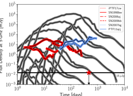
Figure 1.— Template and model 5 GHz light curves of relativistic SNe (red), CSM-interacting SNe (light blue), and off-axis GRBs (grey). All light curves are scaled to $z=0.01$. The red star represents the upper limit derived from the new VLA observation of iPTF17cw presented in Section 2.

Table 1 Summary of light curve templates and models used in this work. Data reported here are taken from: Foley et al. (2006) and Kulkarni et al. (1998) for SN 1998bw; Strauss et al. (1992) anf Soderberg et al. (2010) for SN 2009bb; Sollerman et al. (2006) and Soderberg et al. (2006c) for SN 2006aj; Corsi et al. (2017) for SN iPTF17cw; Adelman-McCarthy et al. (2006) and Corsi et al. (2014) for PTF11qcj; Salas et al. (2013) for SN 2007bg.

	Type	Redshift
SN 1998bw	Rel SN	0.00867
SN 2009bb	Rel SN	0.0099
SN 2006aj	RelSN	0.0331
iPTF 2017cw	Rel SN	0.093
PTF11qcj	CSM-Int SN	0.02811
SN 2007bg	CSM-Int SN	0.0346
E48_theta45	LGRB	-
E49_theta45	LGRB	-
E50_theta45	LGRB	-
E51_theta45	LGRB	-
E52_theta45	LGRB	-
E53_theta45	LGRB	-
E54_theta45	LGRB	-
E48_theta24	LGRB	-
E49_theta24	LGRB	-
E50_theta24	LGRB	-
E51_theta24	LGRB	-
E52_theta24	LGRB	-
E53_theta24	LGRB	-
E54_theta24	LGRB	-

3.1. Radio light curve models and templates

In order to simulate our targets, we use template radio light curves derived from real radio observations of relativistic and CSM-interacting SNe (rescaled at the simulated redshifts and interpolated to the simulated observation time), as well as models for off-axis GRB radio light curves.

For relativistic and CSM-interacting SNe, template and simulated fluxes at specific epochs are derived by performing a linear interpolation between the two closest available data points. If the simulated observing time falls after the time range covered by actual observations of the source, we perform a linear extrapolation of the flux using the last two available observations. This can potentially lead to major errors in the simulated flux if the simulated observing time is far from the last epoch of the actual observations, but we note that this does not happen in the optimized strategy we report in Section 4. Finally, we treat simulated observations at epochs earlier than the first actual observation of a given source in two different ways. First, we assume that these observations result is non detections (i.e., we assume that the simulated flux falls below our sensitivity; see Section 3.2). Next, given uncertainties in the early-time rising behavior of radio SN light curves, we perform early-time extrapolations by assuming a temporal behavior that mimics that of relativistic SNe for which earlier-time observations are actually available (see Section 4.1.1). Results from these two different methods for treating early-time epochs are compared and contrasted to explicitly assess the importance of early-time detections.

To build a set of relativistic SN templates as described above, we use the light curves of SN 1998bw (Kulkarni et al., 1998), SN 2006aj (Soderberg et al., 2006c), SN 2009bb (Soderberg et al., 2010), and iPTF 17cw (Corsi et al., 2017). We choose the first two because they are GRB-associated SNe with well-sampled radio light curves, SN 2009bb because it may represent an event in between GRBs and engine-driven SNe, and iPTF2017cw because it is a relativistic SN located much farther away than the others. SN 1998bw and SN 2009bb were very bright, nearby events visible from few days up to hundreds of days after explosion. They were observed in several radio bands, and here we focus on their detectability at 5 GHz. SN 2006aj was much fainter, it was detected early on, and decayed rapidly until it became too dim after 20 days since explosion. It was observed in several radio bands, but the most complete radio light curve is the one at 8 GHz. For consistency, in our simulations we extrapolated the 8 GHz light curve of SN 2006aj to 5 GHz using a spectral index $\beta$=0.7, typical of optically thin synchrotron emitting sources (e.g., Kellermann, 1964), where we use the convention $F_{\nu}\propto\nu^{-\beta}$. Actual spectral index measurements of SN 2006aj are compatible with this value within large uncertainties (Soderberg et al., 2006c). iPTF 17cw was detected 12 days after explosion, and its 5 GHz light curve also decayed rapidly, with the source becoming undetectable after 30 days. Template radio light curves of relativistic SNe at 5 GHz are plotted in red in Figure 1.

Similarly, we use the measured light curves of PTF 11qcj (Corsi et al., 2014) and SN 2007bg (Salas et al., 2013) as templates for our CSM-interacting SNe. We note that AT 2018cow may be an interesting member of this class of SNe (Margutti et al., 2019). Unfortunately, at the time of writing only a small number of GHz radio detections have been published for this event, so we do not include it here. Template radio light curves of CSM-interacting SNe at 5 GHz are plotted in light blue in Figure 1.

Finally, we simulate 5 GHz radio light curves of off-axis high- and low-luminosity long GRBs using BOXFIT v2 (van Eerten et al., 2012). The BOXFIT light curves depend on several parameters: the luminosity distance ($d_{L}$); the jet half-opening angle ($\theta_{j}$); the viewing angle ($\theta_{v}$); the total explosion energy ($E_{\rm iso}$); the interstellar medium density ($n_{\rm ISM}$); the power-law index of the shocked electrons’ energy distribution $(p)$; and the fraction of the energy converted into magnetic fields and elections ($\epsilon_{B}$ and $\epsilon_{E}$). Here we set $\epsilon_{B}=10^{-2}$, $\epsilon_{E}=10^{-1}$, $\theta_{j}$=12 deg, $p$=2.5 (Ghirlanda et al., 2005; Goldstein et al., 2016; Beniamini & van der Horst, 2017), and $n_{\rm ISM}=1$ cm^-3 (which is the average value found in long GRBs; Chandra & Frail, 2012; Granot & van der Horst, 2014). We create models both using $\theta_{v}=45$ deg, and $\theta_{v}=24$ deg, and varied $E_{\rm iso}$ between $10^{48}$ and $10^{54}$ erg (Frail et al., 2001; Ghirlanda et al., 2004; Amati, 2006; Nava et al., 2012; Perley et al., 2014; Goldstein et al., 2016). These parameters cover both cosmological, more energetic GRBs, and low luminosity ones that are more common in our cosmic neighborhood. The resulting light curves are plotted in grey in Figure 1 (where we neglect redshift corrections).

3.2. Monte Carlo simulations

For each of the targets, we generate 10000 observed light curves drawing from Gaussian distributions with mean equal to the model/template flux at each epoch, and standard deviation equal to the quadrature sum of the error in the template/model and the flux error affecting the simulated observations, $\sqrt{\sigma^{2}_{\rm model/template}+\sigma^{2}_{\rm obs}}$. In the above, $\sigma_{\rm model/template}$ is set to the interpolated measurement errors for our template SN light curves, and to a nominal 10% of the flux for off-axis GRB models; $\sigma_{\rm obs}$ is set to $5\,\mu$Jy, comparable to the image RMS achievable at 5 GHz with the JVLA in its most compact configuration (which provides a conservative estimate of the sensitivity) for a total observing time (including overhead) of 2 hrs per epoch, with $\approx$ 15% bandwidth loss on a nominal 4 GHz bandwidth (3 bit) due to RFI. At any epoch when the simulated model flux is below our detection threshold of $3\times$RMS, the measured flux is set to zero and the error on it is set equal to the noise RMS.

3.3. Optimizing the radio follow-up campaign

We assume that the first radio observation is always carried out as soon as possible, at $t_{\rm radio,0}=t_{\rm opt,0}+\Delta T_{0}$ (having assumed $t=0$ as the time of the SN explosion). Here $t_{\rm opt,0}$ accounts for delay between the SN explosion and the optical discovery. We randomize $t_{\rm opt,0}$ uniformly in the range $1\,{\rm h}-30$ d. $\Delta T_{0}$ allows for a possible further delay between the optical discovery and the earliest radio observation. We tested three different ranges: $\Delta T_{0}=1\,{\rm hr}-2$ d (hereafter dubbed high-urgency follow up), $\Delta T_{0}=3-5$ d (hereafter referred to as medium-urgency follow up), and $\Delta T_{0}=7-15$ d (low urgency).

The ultimate goal of our simulations is to determine the minimum number of radio follow-up observations, $n_{\rm min}$ (where 1$\leq n\leq$10), and their corresponding epochs $\Delta T_{n}=t_{\rm n}-t_{\rm radio,0}=M_{n}\times 2$ d (where $M_{n}$ is an integer in the range $1\leq M_{n}\leq 183$, and its maximum value of 183 is chosen so that all observations happen within one year), required to maximize a figure of merit which we refer to as the number of unique and correct associations, computed as follows.

For each of the simulated observations of target light curves, we determine which templates/models (both targets and contaminants) predict fluxes that at $t_{\rm radio,0}$ agree with the simulated observation within $3\times\sqrt{\sigma^{2}_{\rm model/template}+\sigma^{2}_{\rm obs}}$. These models/templates are considered positive associations for the first epoch, and carried forward to the next observing epoch.

The second epoch can happen with any time delay, $\Delta t_{2}=M_{2}\times 2$ d where $M_{2}=1,2,3,...$, with respect to the first observation. In general, only a subset of the models that represented positive associations for epoch one will also be positive associations for epoch two (i.e. will show agreement between observed flux and predicted model/template flux at that epoch within $3\times\sqrt{\sigma^{2}_{\rm model}+\sigma^{2}_{\rm obs}}$). Thus, we optimize the value of $M_{2}$ by maximizing the number of associations that in epoch two become unique (only one model/template fits the observed target in both epochs) and correct (the model/template that fits the observations uniquely is also the correct one, i.e. it is the same template/model from which the observations were simulated).

We then add a third observing epoch, keeping the two already analyzed in place. As before, the third epoch can happen with any time delay, $\Delta t_{3}=M_{3}\times 2$ d where $M_{3}=1,2,3,...$, with respect to the first observation. So we optimize $M_{3}$ by maximizing the number of associations that, after being positive in both epoch one and two, become unique and correct identifications in epoch three.

We keep repeating this process until we reach a maximum of ten epochs. Naturally, adding more observational epochs will progressively increase the fraction of unique and correct associations up to that epoch. Note that it may happen that in the optimization process $M_{n}$ turns out to be larger than $M_{n+1}$. Thus, the times of the optimized observational epochs are ordered in increasing delays since first epoch once the optimization process is completed, as presented in Tables 2, 3, and 4.

4. Results

4.1. Discovering relativistic SNe

Our goal here is to optimize the observational strategy to detect relativistic, engine-driven SNe in the radio. For this reason, we treat the relativistic SN templates listed in Table 1 as our targets, while CSM-interacting SNe and off-axis GRBs are treated as contaminants. Targets that are not detectable because always too faint at the considered redshift are excluded from this analysis (i.e., they are not considered when calculating the efficiency of our strategies) A summary of our results is reported in Table 2. We find that five observations are required in order to maximize the number of unique and correct associations. In terms of urgency, we find the largest number of unique and correct associations when adopting a high-urgency strategy, i.e., minimum interval between the optical discovery and the first radio observation (see Section 3.3).

At $z=0.01$, 95% of the simulated targets are detectable, and 97% of the detectable targets are uniquely and correctly associated. All targets simulated from the templates of SN 1998bw, SN 2009bb and iPTF 17cw, and 80% of SN 2006aj are detectable. 100% of the detectable targets simulated from the templates of SN 1998bw, SN 2009bb and iPTF 17cw, and 84% of SN 2006aj are uniquely and correctly associated. Missed associations are due the fact that SN 2006aj is very faint and faded away quickly.

For sources at $z=0.1$, we have much fewer unique and correct associations, especially for targets whose peak flux was close to our detection limit at $z=0.01$ (e.g., SN 2006aj-like sources). In fact, the fraction of detected sources drops to 72%, and 78% of those sources is uniquely and correctly associated. In particular, 100% of the targets simulated from the templates of SN 1998bw and SN 2009bb, 19% of SN 2006aj, and 71% of iPTF 17cw are detectable. Of those, 100% of the targets simulated from the templates of SN 1998bw and SN 2009bb, 0% of SN 2006aj, and 36% of iPTF 17cw are uniquely and correctly associated. For sources at $z=0.1$ the difference between different urgency strategies is negligible. This is likely due to the fact that at this distance the early, rising part of the light curve falls below our detection threshold, thus having early observations would not particularly affect the results. Missed associations in this case are due the fact that the light curve iPTF 17cw is not well sampled at early times. Our discussion in Section 4.1.1 clarifies this point.

In the case of sources with redshift randomly distributed between 0.01 and 0.1 our results are, as expected, in between the two previously described cases. Specifically, 92% of all simulated sources are detected, and 87% of the detected sources are uniquely and correctly associated. In particular, 100% of the targets simulated from the templates of SN 1998bw and SN 2009bb, 69% of SN 2006aj, and 99% of iPTF 17cw are detected. Of those detected sources, 100% of the targets simulated from the templates of SN 1998bw and SN 2009bb, 48% of SN 2006aj, and 88% of iPTF 17cw are uniquely and correctly associated.

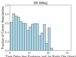
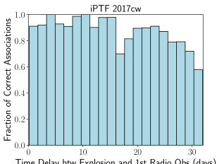
Figure 2.— Fraction of targets that are uniquely and correctly associated as a function of the total delay between the SN explosion and the first radio observation for sources with $z=0.01-0.1$.

For completeness, in Figure 2 we also plot the the efficiency of the optimized observing campaign as a function of total time delay for SN 2006aj-like and PTF17cw-like targets, with redshifts randomly distributed between 0.01 and 0.1. The total time delay is calculated as the sum of the delay between the explosion and the optical detection, and the delay between the optical detection and the first radio observation (which defines the urgency of the radio observing campiagn; see Section 3.3). In this Figure the efficiency (fraction of unique and correct associations) is calculated relative to the number of simulated sources that are detected in each delay bin. We note that for SN 1998bw-like and SN 2009bb-like targets, the efficiency is 100% regardless of the total time delay (and thus, regardless of the adopted observing urgency strategy in the radio). In the case of SN 2006aj-like targets, we completely miss those that are observed with total delays $\gtrsim 22$ d, when SN 2006aj was undetected.

Table 2 Summary of our results for relativistic SNe. The efficiency quoted here is the average among all relativistic SNe listed in Table 1, for a high-urgency follow-up strategy. Targets that are not detectable have been excluded from this analysis. See text for discussion.

$z$	Efficiency	days since 1st obs.
0.01	97%	2, 8, 18, 30
0.1	78%	2, 6, 18, 34
Mix	87%	4, 10, 22, 30

4.1.1 Relevance of early-time radio observations for relativistic SNe

In this Section we assess the importance of early-time radio observations for correctly and uniquely associating relativistic SNe via an optimized radio follow-up campaign. To this end, we extrapolate the template light curves of SN 2009bb and iPTF 17cw using the early-time behavior of the much better sampled radio light curves of SN 1998bw and SN 2006aj, respectively. We choose to use SN 1998bw to extrapolate the light curve of SN 2009bb, and SN 2006aj to extrapolate the light curve of iPTF 17cw, because they are the most similar to each other. In fact, both SN 1998bw and SN 2009bb were nearby explosions that resulted in a very bright radio signal. On the other hand, both SN 2006aj and iPTF 17cw were very dim and faded away very rapidly.

We repeat the simulations and optimization procedure described in the previous Section including these early-time extrapolations. Since all sources simulated based on the template of SN 2009bb were both detected and correctly and uniquely associated without this early-time extrapolation, we do not expect significant changes in the results for SN 2009bb-like sources. On the other hand, we do expect an improvement in the results for iPTF 17cw-like SNe, specifically for the cases of $z=0.1$ and mixed redshifts (since all iPTF 17cw-like sources were detected, and correctly and uniquely associated, at $z=0.01$).

A summary of the results from this analysis, averaged over all the relativistic SN templates, is reported in Table 3, and confirm our expectations. Specifically for iPTF 17cw-like targets at $z=0.1$, 95% are detected, and 64% of those are correctly and uniquely associated. For mixed redshifts, all of the iPTF 17cw-like sources are detected, and 95% of them are correctly and uniquely associated. These results highlight the need for early-time radio observations of newly-discovered relativistic SNe. Not only a high-urgency strategy is indeed favored for triggering the first radio observation, but all of the follow-up campaign should be conducted within the first 2-3 weeks since explosion.

Table 3Summary of our results for relativistic SNe when extrapolating the light curves of SN 2009bb and iPTF 17cw to early times, as explained in Section 4.1.1. The efficiency quoted here is the average among all relativistic SNe listed in Table 1, for a high-urgency follow-up strategy. Targets that are not detectable have been excluded from this analysis. See text for discussion.

$z$	Efficiency	days since 1st obs.
0.01	97%	4, 8, 14, 22
0.1	83%	2, 6, 14, 18
Mix	91%	2, 4, 8, 10

4.2. Discovering CSM-interacting SNe

Our goal here is to optimize the observational strategy to detect CSM-interacting SNe in the radio. For this reason, we treat the CSM-interacting SN templates listed in Table 1 as our targets, while relativistic SNe and off-axis GRBs are treated as contaminants.

The earliest detection for both our CSM-interacting templates happened around 30 d after the explosion. It is therefore expected that, in terms of urgency, we would find the highest number of positive identifications when adopting a low-urgency radio follow-up, i.e., the largest interval between the optical discovery and the first radio observation (see Section 3.1 for how we extrapolate template fluxes at epochs preceding the earliest detection). Moreover, as evident from Figure 1, the radio light curves of CSM-interacting SNe start diverging from the light curves of other contaminants around 40-70 d after the explosion, so one can already expect that observations after these epochs (which correspond to about 30-60 d after the first radio observation) would be optimal.

We run our simulations with the same redshift intervals as for relativistic SNe in Section 4.1. Results are reported in Table 4. In this case, we find that three epochs of radio follow-up observations are sufficient to correctly and uniquely identify all of the simulated sources, and that using a low-urgency strategy suffices. Overall, the optimal radio follow-up strategy for CSM-interacting SNe requires observations at later times than relativistic SNe. However, we also stress that the results reported here are subject to uncertainties related to the limited number of radio-emitting, CSM-interacting BL-Ic SNe we know of so far. More discoveries of this type of explosions in the future will enable us to better refine radio follow-up strategies.

Table 4Summary of our results for CSM-interacting SNe. The efficiency quoted here is the average among all CSM-interacting SNe listed in Table 1, for a low-urgency follow-up strategy. Targets that are not detectable have been excluded from this analysis. See text for discussion.

$z$	Efficiency	days since 1st obs.
0.01	100%	6, 90
0.1	100%	22, 90
Mix	100%	6, 90

4.3. Discovering Off-Axis GRBs

In this last Section our goal is to optimize the observational strategy to detect off-axis long GRBs. We therefore treat the off-axis GRB models listed in Table 1 as our targets, while relativistic SN and the CSM-interacting SN templates are treated as contaminants. As can be seen from Figure 1, off-axis GRB models span a variety of fluxes and timescales, and by construction are much better sampled than our other SN templates at early and late times. Thus, we generally expect that a large fraction of the detectable sources will also be be uniquely and correctly identified. However, we note that not all off-axis GRB models are detectable at all distances. In particular, the peak flux of the E48_theta45 model is below the radio detection threshold even at $z=0.01$. Moreover, the peak fluxes of the E49_theta45 and the E48_theta24 models are barely above the radio detection threshold for a short time, so the radio follow-up efficiency is largely dominated by the delay between explosion and optical discovery.

Results of our simulations are reported in Table 5. We find that five epochs are necessary to maximize the amount of correct and unique associations, and that a high-urgency strategy is preferable, especially for the low luminosity GRBs ($E_{\rm iso}<10^{51}\,$erg).

At $z=0.01$, overall 82% of sources are detected. In particular, 3% of E48_theta24, 23% of E49_theta24, and 39% of E49_theta45 are detected. The fact, for sources with $E_{\rm iso}=10^{49}\,$erg, the case $\theta_{v}$=45 deg yields to more detections than $\theta_{v}$=24 deg is explained by the faster evolution of E49_theta24 which, in spite of having a peak flux brighter than E49_theta45, becomes quickly undetectable after less than 6 days since explosion. For all other GRB model parameters, all sources are detected at $z=0.01$. Overall, 99% of the off-axis GRBs detected at $z=0.01$ are uniquely and correctly associated. Specifically, unique and correct association efficiencies are 100% for $E_{\rm iso}>10^{51}\,$erg, 81% for E48_theta24, 90% for E49_theta24, 99% for E50_theta24, 96% for E49_theta45, and 100% for E50_theta45.

At $z=0.1$, overall 63% of off-axis GRBs are detected. All explosions with $E_{\rm iso}>10^{51}\,$erg are always detectable; 25% of E50_theta24 are detectable; while sources with $E_{\rm iso}\leq 10^{50}\,$erg and $\theta_{v}$=45 deg, and sources with $E_{\rm iso}\leq 10^{49}\,$erg and $\theta_{v}$=24 deg are never detectable at this redshift. Overall, of the detectable sources at $z=0.1$, 96% are uniquely and correctly associated. Specifically, unique and correct association efficiencies are of 100% for all detectable sources with $\theta_{v}$=45 deg, 4% for E50_theta24, 91% for E51_theta24, and 100% for explosions with $E_{\rm iso}>10^{52}\,$erg.

Finally, in the case of sources with redshift randomly distributed between 0.01 and 0.1 our results are, as expected, in between the two previously described cases. Overall, 73% of the off-axis GRBs are detected. More specifically, 100% of $E_{\rm iso}>10^{51}\,$erg, 0.4% of E48_theta24, 9% of E49_theta24, 58% of E50_theta24, 9% of E49_theta45, and 70% of E50_theta45 are detected. Overall, 96% of the detectable off-axis GRBs with mixed redshifts are uniquely and correctly associated. In particular, unique and correct association efficiencies are as follows: 100% for $E_{\rm iso}>10^{52}\,$erg, 77% for E48_theta24, 73% for E49_theta24, 73% for E50_theta24, 98% for E51_theta24, 68% for E49_theta45, 78% for E50_theta45, and 100% for E51_theta45.

Table 5Summary of our results for off-axis GRBs. The efficiency quoted here is the average among all off-axis GRB models listed in Table 1, for a high-urgency strategy. Targets that are not detectable have been excluded from this analysis. See text for discussion.

$z$	Efficiency	days since 1st obs.
0.01	99%	6, 22, 26, 82
0.1	96%	10, 14, 26, 82
Mix	96%	4, 10, 26, 82

5. Detectability in X-rays

Hereafter we consider the benefits of X-ray follow-up observations of both relativistic SNe and CSM-interacting SNe, and the potential for X-ray detections. Radio and X-ray observations both probe the fastest component of the SN ejecta. Combining radio and X-ray data one can independently constrain the density of the medium ($n_{\rm ISM}$) and the fraction of ejecta energy converted in magnetic fields ($\epsilon_{\rm B}$; Chevalier & Fransson, 2006).

We estimate the X-ray flux of our targets at the time of the radio peak, assuming the X-rays are produced via synchrotron emission with radio-to-X-ray spectrum defined as follows:

$$F_{X}=F_{\rm radio}\times\left(\frac{\nu_{X}}{\nu_{\rm radio}}\right)^{-\beta},$$ (1)

where $F_{X}$ and $F_{\rm radio}$ are the fluxes in the X-ray and radio bands respectively, $\nu_{\rm X}$ and $\nu_{\rm radio}$ are the frequencies of the X-ray and radio observations respectively, and $\beta\approx 0.7-1$ is the spectral index.

We test the detectability of the X-ray emission from our sources with both Swift and Chandra. For what concerns X-ray observations with Swift, in a $\sim$10 ks-long observation one can reach a 3$\sigma$ sensitivity of $\sim$2.5$\times$10^-14 erg cm^-2 s^-1 (unabsorbed flux; Gehrels et al., 2004). With $\beta$=1, all sources would be too dim to be detectable. On the other hand, with $\beta$=0.7, all sources would be detectable at $z=0.01$, but none would be detectable at $z=0.1$. With a 20 ks-long observation with Chandra one could reach a 3$\sigma$ sensitivity of $\sim$3$\times$10^-15 erg cm^-2 s^-1 (unabsorbed flux; Burrows et al., 2005). In this case, with $\beta$=1, only SN 1998bw, SN 2009bb, PTF 2011qcj, and SN 2007bg would be detectable at $z=0.01$, while none would be at $z=0.1$. With $\beta$=0.7, all sources would be detectable even at $z=0.1$, although SN 2006aj and PTF 2017cw would be very close to the detection threshold.

We also calculate for how long the X-ray emission would be detectable by Chandra. Our results are reported in Table 6. These results assume that, during the whole time, the X-ray emission is produced via synchrotron radiation with a constant radio-to-X-ray spectral index as in Equation 1. We note that for all sources, with $\beta$=0.7 and $z$=0.01, the X-ray emission would be visible at least as long as we have radio observations of the sources.

We finally calculate the distance limit (i.e. the distance at which the flux would be equal to the sensitivity limit of Chandra) for each source. Our results are reported in Table 7. We highlight that the distance limits derived for SN 2006aj-like and iPTF17cw-like SNe in the case $\beta$=1 are closer than the actual distance to these sources, despite both of them were detected in X-rays (Campana et al., 2006; Corsi et al., 2017). This is explained by the fact that evidence for a flattening of the radio-to-X-ray spectral index, possibly related to cosmic-ray dominated shocks, has been observed in these events (Ellison et al., 2000; Chevalier & Fransson, 2006; Vink, 2017). The distance limit we obtain for SN 2007bg is also closer than the source’s actual distance (152 Mpc), in agreement with the fact that no X-ray detection was reported ($F_{X}<2.6\times 10^{-15}$ erg cm^-2 s^-1; Salas et al., 2013).

Table 6 Maximum time after explosion at which X-ray emission would be detectable in a 20 ks-long observation with Chandra. We assume X-rays are produced via synchrotron emission with constant radio-to-X-ray spectral index in the range $\beta\approx 0.7-1$ over these timescales. The first entry corresponds to the case $\beta=0.7$, while the second to $\beta=1$. A forward slash indicates that a source is never detectable. A greater than ($>$) symbol indicates that the source is detectable at least until the time of the latest radio observation we considered. See text for discussion.

Source	$\Delta t_{{\rm max},z=0.01}$	$\Delta t_{{\rm max},z=0.1}$
	(days)	(days)
SN 1998bw	$>250-\sim 70$	$\sim 90-/$
SN 2009bb	$>150-\sim 70$	$\sim 100-/$
SN 2006aj	$>22-/$	$\sim 5-/$
iPTF 17cw	$>31-/$	$\sim 16-/$
PTF 11qcj	$>600->600$	$>600-/$
SN 2007bg	$>860->860$	$>860-/$

Table 7Distance at which the X-ray flux of both relativistic and CSM-interacting SNe would be equal to the $3\sigma$ sensitivity limit of a 20 ks-long observation with Chandra, assuming the radio-to-X-ray emission is synchrotron radiation with no spectral breaks and $\beta\approx 0.7-1$. The first entry corresponds to the case $\beta=0.7$, while the second to $\beta=1$. See text for discussion.

Source	Horizon
	(Mpc)
SN 1998bw	1634-104
SN 2009bb	950-60
SN 2006aj	525-33
iPTF 17cw	567-36
PTF11qcj	1853-117
SN 2007bg	1467-93

6. Summary and conclusion

We have presented an analysis aimed at identifying an optimal strategy for detecting and characterizing various types of radio-emitting stripped-envelope core-collapse SNe with the VLA.

Our results show how early-time ($<$7 days after the explosion) radio observations are key to identifying relativistic, engine-driven SNe, whose radio emission peaks early and fades away quickly. This is clearly demonstrated by our results for SN 2009bb-like and iPTF 17cw-like explosions. Radio emission from CSM-interacting SNe is typically longer-lived, and can successfully be identified via later times observations, around 40-90 days after the explosion, although this conclusion is affected by uncertainties related to the limited number of radio-emitting, CSM-interacting BL-Ic SNe we know of so far. For radio afterglows of off-axis long GRBs, early-time observations are required in order to maximize the probability of correctly interpreting their origin and physical properties.

Finally, we discussed the detectability of relativistic and CSM-interacting SNe in X-rays. We found that, if their X-ray emission is due to synchrotron radiation, most of them are only detectable when they are relatively nearby ($<$100 Mpc) for spectral indices greater than unity, while they may be detected up to about 1 Gpc for spectral indices of about 0.7.

In the near future, LSST will discover about $10^{4}$ BL-Ic SNe per year (LSST Science Collaboration et al., 2009; Shivvers et al., 2017), providing a fantastic resource to investigate the fraction of these events linked to long GRBs. Utilizing an optimized strategy to follow-up BL-Ic SNe in the radio will be crucial to investigate as many events as possible, and put tighter constraints on the open question of the nature of their progenitors. At the time LSST will be starting operations (mid-late 2020s), a next generation Very Large Array (ngVLA) will likely be starting operations as well (Murphy et al., 2018). ngVLA is a proposed next generation radio interferometer with $\approx 10\times$ the sensitivity of the current VLA, which will enable discovery of sources $\approx 3\times$ as far, therefore enlarging the number of possible detections by about a factor of 30, and dramatically expanding the capabilities to discover new radio-loud SNe of the rarest types.

References

- Adelman-McCarthy et al. (2006) Adelman-McCarthy, J. K., Agüeros, M. A., Allam, S. S., et al. 2006, ApJS, 162, 38
- Amati (2006) Amati, L. 2006, MNRAS, 372, 233
- Amati et al. (2002) Amati, L., Frontera, F., Tavani, M., et al. 2002, A&A, 390, 81
- Bellm (2016) Bellm, E. C. 2016, PASP, 128, 084501
- Beniamini & van der Horst (2017) Beniamini, P., & van der Horst, A. J. 2017, MNRAS, 472, 3161
- Berger et al. (2003) Berger, E., Kulkarni, S. R., Frail, D. A., & Soderberg, A. M. 2003, ApJ, 599, 408
- Bromberg et al. (2011) Bromberg, O., Nakar, E., & Piran, T. 2011, ApJ, 739, L55
- Burrows et al. (2005) Burrows, D. N., Hill, J. E., Nousek, J. A., et al. 2005, Space Sci. Rev., 120, 165
- Campana et al. (2006) Campana, S., Mangano, V., Blustin, A. J., et al. 2006, Nature, 442, 1008
- Carbone & Corsi (2018) Carbone, D., & Corsi, A. 2018, ApJ, 867, 135
- Chandra & Frail (2012) Chandra, P., & Frail, D. A. 2012, ApJ, 746, 156
- Chevalier & Fransson (2006) Chevalier, R. A., & Fransson, C. 2006, ApJ, 651, 381
- Corsi et al. (2011) Corsi, A., Ofek, E. O., Frail, D. A., et al. 2011, ApJ, 741, 76
- Corsi et al. (2014) Corsi, A., Ofek, E. O., Gal-Yam, A., et al. 2014, ApJ, 782, 42
- Corsi et al. (2016) Corsi, A., Gal-Yam, A., Kulkarni, S. R., et al. 2016, ApJ, 830, 42
- Corsi et al. (2017) Corsi, A., Cenko, S. B., Kasliwal, M. M., et al. 2017, ApJ, 847, 54
- Eichler & Levinson (1999) Eichler, D., & Levinson, A. 1999, ApJ, 521, L117
- Ellison et al. (2000) Ellison, D. C., Berezhko, E. G., & Baring, M. G. 2000, ApJ, 540, 292
- Filippenko (1997) Filippenko, A. V. 1997, ARA&A, 35, 309
- Foley et al. (2006) Foley, S., Watson, D., Gorosabel, J., et al. 2006, A&A, 447, 891
- Frail et al. (2001) Frail, D. A., Kulkarni, S. R., Sari, R., et al. 2001, ApJ, 562, L55
- Gal-Yam (2017) Gal-Yam, A. 2017, Observational and Physical Classification of Supernovae, 195
- Galama et al. (1998) Galama, T. J., Vreeswijk, P. M., van Paradijs, J., et al. 1998, Nature, 395, 670
- Gehrels et al. (2004) Gehrels, N., Chincarini, G., Giommi, P., et al. 2004, ApJ, 611, 1005
- Ghirlanda et al. (2005) Ghirlanda, G., Ghisellini, G., & Firmani, C. 2005, MNRAS, 361, L10
- Ghirlanda et al. (2004) Ghirlanda, G., Ghisellini, G., & Lazzati, D. 2004, ApJ, 616, 331
- Goldstein et al. (2016) Goldstein, A., Connaughton, V., Briggs, M. S., & Burns, E. 2016, ApJ, 818, 18
- Graham et al. (2019) Graham, M. J., Kulkarni, S. R., Bellm, E. C., et al. 2019, PASP, 131, 078001
- Granot & van der Horst (2014) Granot, J., & van der Horst, A. J. 2014, PASA, 31, e008
- Ho et al. (2019) Ho, A. Y. Q., Goldstein, D. A., Schulze, S., et al. 2019, arXiv e-prints, arXiv:1904.11009
- Kellermann (1964) Kellermann, K. I. 1964, ApJ, 140, 969
- Kulkarni et al. (1998) Kulkarni, S. R., Frail, D. A., Wieringa, M. H., et al. 1998, Nature, 395, 663
- Law et al. (2009) Law, N. M., Kulkarni, S. R., Dekany, R. G., et al. 2009, PASP, 121, 1395
- LSST Science Collaboration et al. (2009) LSST Science Collaboration, Abell, P. A., Allison, J., et al. 2009, arXiv e-prints, arXiv:0912.0201
- Margutti et al. (2019) Margutti, R., Metzger, B. D., Chornock, R., et al. 2019, ApJ, 872, 18
- Mazzali et al. (2014) Mazzali, P. A., McFadyen, A. I., Woosley, S. E., Pian, E., & Tanaka, M. 2014, MNRAS, 443, 67
- McMullin et al. (2007) McMullin, J. P., Waters, B., Schiebel, D., Young, W., & Golap, K. 2007, in Astronomical Society of the Pacific Conference Series, Vol. 376, Astronomical Data Analysis Software and Systems XVI, ed. R. A. Shaw, F. Hill, & D. J. Bell, 127
- Murphy et al. (2018) Murphy, E. J., Bolatto, A., Chatterjee, S., et al. 2018, in Astronomical Society of the Pacific Conference Series, Vol. 517, Science with a Next Generation Very Large Array, ed. E. Murphy, 3
- Nava et al. (2012) Nava, L., Salvaterra, R., Ghirlanda, G., et al. 2012, MNRAS, 421, 1256
- Palliyaguru et al. (2019) Palliyaguru, N. T., Corsi, A., Frail, D. A., et al. 2019, ApJ, 872, 201
- Perley et al. (2014) Perley, D. A., Cenko, S. B., Corsi, A., et al. 2014, ApJ, 781, 37
- Perna & Loeb (1998) Perna, R., & Loeb, A. 1998, ApJ, 509, L85
- Piran (2004) Piran, T. 2004, Reviews of Modern Physics, 76, 1143
- Prentice et al. (2018) Prentice, S. J., Maguire, K., Smartt, S. J., et al. 2018, ApJ, 865, L3
- Rhoads (1997) Rhoads, J. E. 1997, ApJ, 487, L1
- Salas et al. (2013) Salas, P., Bauer, F. E., Stockdale, C., & Prieto, J. L. 2013, MNRAS, 428, 1207
- Shivvers et al. (2017) Shivvers, I., Modjaz, M., Zheng, W., et al. 2017, PASP, 129, 054201
- Smith et al. (2014) Smith, R. M., Dekany, R. G., Bebek, C., et al. 2014, in Proc. SPIE, Vol. 9147, Ground-based and Airborne Instrumentation for Astronomy V, 914779
- Soderberg et al. (2006a) Soderberg, A. M., Chevalier, R. A., Kulkarni, S. R., & Frail, D. A. 2006a, ApJ, 651, 1005
- Soderberg et al. (2006b) Soderberg, A. M., Nakar, E., Berger, E., & Kulkarni, S. R. 2006b, ApJ, 638, 930
- Soderberg et al. (2006c) Soderberg, A. M., Kulkarni, S. R., Nakar, E., et al. 2006c, Nature, 442, 1014
- Soderberg et al. (2010) Soderberg, A. M., Chakraborti, S., Pignata, G., et al. 2010, Nature, 463, 513
- Sollerman et al. (2006) Sollerman, J., Jaunsen, A. O., Fynbo, J. P. U., et al. 2006, A&A, 454, 503
- Strauss et al. (1992) Strauss, M. A., Huchra, J. P., Davis, M., et al. 1992, ApJS, 83, 29
- van Eerten et al. (2012) van Eerten, H., van der Horst, A., & MacFadyen, A. 2012, ApJ, 749, 44
- Vink (2017) Vink, J. 2017, X-Ray Emission Properties of Supernova Remnants, ed. A. W. Alsabti & P. Murdin, 2063
- Waxman (2004) Waxman, E. 2004, ApJ, 602, 886
- Woosley & Bloom (2006) Woosley, S. E., & Bloom, J. S. 2006, ARA&A, 44, 507
- Yamazaki et al. (2003) Yamazaki, R., Yonetoku, D., & Nakamura, T. 2003, ApJ, 594, L79