A Symbolic Neural Network Representation and its Application to Understanding, Verifying, and Patching Networks

Abstract.

Analysis and manipulation of trained neural networks is a challenging and important problem. We propose a symbolic representation for piecewise-linear neural networks and discuss its efficient computation. With this representation, one can translate the problem of analyzing a complex neural network into that of analyzing a finite set of affine functions. We demonstrate the use of this representation for three applications. First, we apply the symbolic representation to computing weakest preconditions on network inputs, which we use to exactly visualize the advisories made by a network meant to operate an aircraft collision avoidance system. Second, we use the symbolic representation to compute strongest postconditions on the network outputs, which we use to perform bounded model checking on standard neural network controllers. Finally, we show how the symbolic representation can be combined with a new form of neural network to perform patching; i.e., correct user-specified behavior of the network.

1. Introduction

1.1. Introduction to Neural Networks

The past decade has seen the rise of deep neural networks (DNNs) (Goodfellow et al., 2016) to solve a variety of problems, including image recognition (Szegedy et al., 2016; Krizhevsky et al., 2017), natural-language processing (Devlin et al., 2018), and autonomous vehicle control (Julian et al., 2018). Typically, DNNs are trained using large data sets, validated on a test set, and then deployed. As they permeate more and more systems, there is growing need for tools to more deeply analyze and modify such networks once they have been trained. This paper presents techniques for understanding, verifying, and patching (correcting) trained neural networks. These various applications rely on a new symbolic representation of neural networks introduced in this paper.

In this work, we focus on the major class of piecewise-linear neural networks, which can be decomposed into a set of affine functions (Definition 1). For example, the function $\max(x,0)$ is piecewise-linear; when $x\leq 0$ it takes the affine form $x\mapsto 0$, and when $x>0$ it takes the affine form $x\mapsto x$. Although this may seem like a restrictive definition, we will show in Section 3 that neural networks using the most common building blocks (like 2DConvolution, ReLU, and MaxPool layers) are in fact piecewise-linear. Notably, this work deals with trained networks (we assume that the training has been already been completed), and makes no restriction on the training process.

1.2. Contributions

A symbolic representation for deep neural networks.  In Section 3, we propose a symbolic representation for neural networks which expresses a complex, highly-non-linear neural network in terms of a set of affine functions, each of which fully captures the behavior of the network for a particular subspace of the input domain. We refer to this subspace as the restriction domain of interest, and consider in this work two-dimensional restriction domains of interest, which we show in Section 8 leads to many important applications. Fundamentally, this representation allows us to translate questions about the highly-non-linear neural network into a series of questions about finitely-many affine functions, which are one of the best-studied class of functions in modern mathematics. As we will see, this symbolic representation enables understanding, verifying, and patching trained neural networks.

Understanding network behavior using weakest precondition.  In Section 5, we show how the symbolic representation can be used to compute weakest preconditions on neural networks; i.e., all points in the input space which are mapped to a particular subset of the output space by the network. We show that prior work can be adapted to compute preconditions, but they are not guaranteed to produce the weakest precondition (i.e., they produce a subset of the points). This weakest-precondition primitive allows us to understand the behavior of a neural network by exactly visualizing decision boundaries. In particular, we apply this technique to the aircraft collision avoidance system ACAS Xu (Julian et al., 2018), comparing the use of the proposed symbolic representation to prior work based on an (over-approximating) abstraction of the network function.

In Section 8.1 we use the preconditions to plot network decision boundaries, and compare against the preconditions found using a representation from prior work. We find that the representations in prior work are not precise enough to compute particularly useful preconditions, whereas the representation used in this work can find weakest preconditions in a matter of seconds.

Bounded model checking of safety properties using strongest postcondition.  In Section 6, we show how the symbolic representation can be adapted to compute strongest post-conditions on the network output, i.e. all outputs reachable by the network from a set of inputs.

In Section 8.2, we use this to perform bounded model checking (Biere et al., 2009) on three reinforcement learning controller models, comparing against the state-of-the-art neural network SMT solver ReluPlex (Katz et al., 2017). We find that the ability to directly handle disjunctions as well as re-use information across multiple verification steps allows the proposed technique to verify significantly more steps in the same time limit (including finding a counter-example to the safety specification for one of the models).

Patching deep neural networks.  In Section 7, we consider the problem of patching a neural network: changing a small number of weights in the network to precisely manipulate the network decision boundaries (eg. to fix erroneous or undesired behavior). Three features in particular make this a challenging problem:

1. Neural networks are usually high-dimensional and highly non-linear, pushing the bounds of traditional SMT solvers such as Z3 (de Moura and Bjørner, 2008).

2. The behavior we would like to patch occurs over entire polytopes (containing infinitely many points) in the input region, making it difficult to apply gradient-descent-based methods which assume a finite set of training points.

3. One may not have the original training or test data for a network (eg. due to user privacy concerns), making it difficult to ensure that applying a patch to fix one set of erroneous behavior does not result in corrupting the behavior for another set of inputs.

We discuss prior work that relies on over-approximations and/or differentiable relaxations, but find them sub-optimal for this particular problem. We then define a new class of neural networks termed Masking Networks (Section 7.2), and show how standard networks can be transformed into equivalent Masking Networks. Finally, we show how our symbolic representation can be used on such networks to lower the problem of patching on polytopes to that of patching on a finite set of vertices, intuitively similar to how the simplex algorithm lowers optimization over a polytope to optimization over a finite set of vertices. These changes allow us to rephrase the problem of patching as solving a finite MAX SMT problem. We discuss a number of approaches to this problem, including using the Z3 theorem prover (de Moura and Bjørner, 2008), which we find to be too slow for our purposes. We then discuss an algorithm that can exactly and efficiently solve such problems when only a single weight is changed. Finally, we greedily apply that solver to find better solutions by changing multiple weights.

In Section 8.3 we test this network patching technique on an aircraft collision-avoidance network with three patch specifications. We show quantitatively and qualitatively that patching is effective even with relatively few iterations. We also find that patches made to one restriction domain of interest can have beneficial effects on others (i.e., patches generalize).

Section 2 presents an overview of the symbolic representation and its applications, while Section 9 describes related work and Section 10 summarizes the main results of this paper.

2. Overview

2.1. Deep Neural Networks and Piecewise-Linear Functions

Deep neural networks (Goodfellow et al., 2016) generally consist of multiple layers (which are themselves vector-valued functions) applied sequentially to an input vector. Thus, a DNN can be thought of as a function $f=f_{n}\circ f_{n-1}\circ\cdots\circ f_{1}$, where $f_{i}$ is function representing the $i$th layer. Four layer types are particularly common in feed-forward neural networks:

1. FullyConnected layers correspond to arbitrary affine maps, where the particular map is determined by the weight matrix of the layer.

2. 2DConvolution layers correspond to a restricted subset of affine maps particularly well-suited to image recognition and parameterized by a filter tensor.

3. ReLU layers effectively enforce a lower-bound on the value of each coefficient in the output vector. If the output of the previous layer was $x$, then $\textsc{ReLU}{}(x)_{i}=0$ when $x_{i}\leq 0$ and $x_{i}$ when $x_{i}>0$ (where $\textsc{ReLU}{}(x)_{i}$ is the $i$th component of the layer’s output vector). For example, $\textsc{ReLU}{}((10,-2))=(10,0)$.

4. MaxPool layers condense their input vectors by taking only the maximum value in each of a number of coefficient groups.

5. BatchNorm layers normalize each component given a fixed mean and variance.

Of particular importance to our paper, all of these layers are examples of piecewise-linear functions:

Definition 1.

A function $f:A\to B$ is referred to as a piecewise-linear function if its input domain $A$ can be partitioned by a finite set of (possibly unbounded) convex polytopes $\{P_{1},P_{2},\ldots,P_{n}\}$ such that, within any partition $P_{i}\subseteq A$, there exists an affine map $F_{i}:P_{i}\to B$ satisfying $f(x)=F_{i}x$ for any $x\in P_{i}$.

In other words, each layer function can be broken up into finitely many affine functions, with one of those functions being applied depending on the location in the input space of $x$. For example, the ReLU function, when restricted to any one orthant (i.e., where the signs of all input coefficients are constant), corresponds to a single affine map that zeros out entries with a non-positive sign. Because (1) there are finitely many orthants that together partition the input space, (2) each orthant can be expressed as a convex polytope, and (3) within each orthant $\textsc{ReLU}{}(x)$ is affine, we can say that ReLU is a piecewise-linear function.

2.2. Restriction Domains of Interest

Figure 1. An illustration of restriction domain of interest. The function $f$ has a three-dimensional domain and ${f}_{\restriction X}$ is $f$ restricted to a particular two-dimensional restriction domain of interest $X$.

One particular insight which we will utilize throughout the paper is that, when analyzing networks, one is usually only interested in a particular domain of interest. For example, suppose a network $f:\mathbb{R}^{2}\to\mathbb{R}^{1}$ predicts the probability of acquiring cancer in the next five years, taking as input a vector with two components, $x=(x_{1},x_{2})$, with $x_{1}$ being the age of the patient and $x_{2}$ being the percent of their immediate family that has died of cancer. Then, although $f$ is theoretically able to make predictions about, say, $1,000$-year-old individuals with $110\%$ of their immediate family having died of cancer, such scenarios are in practice impossible. Furthermore, in particular scenarios, we may be concerned with an even smaller subspace of the input domain, for example if we only want to understand how the network classifies children under the age of $10$.

We call such restricted subsets of the input domain the restriction domain of interest for the particular analysis being performed, usually denoted by $X$, and to indicate that we only intend to consider the behavior over the restriction domain of interest, we will often write ${f}_{\restriction X}$ (read “$f$ restricted to the restriction domain of interest $X$”). This is illustrated in Figure 1, where a function with a three-dimensional domain is restricted to a particular two-dimensional restriction domain of interest. In Section 4.3 we will focus on two-dimensional restriction domains of interest, which we will show can help significantly improve the efficiency of our analysis.

Definition 2.

A function $f:A\to B$ restricted to a particular restriction domain of interest $X\subseteq A$, denoted ${f}_{\restriction X}$, is a new function ${f}_{\restriction X}:X\to B$ such that ${f}_{\restriction X}(x)=f(x)$ for any $x\in X$.

2.3. A Symbolic Representation for Deep Neural Networks

In this work, we develop a symbolic representation for a deep neural network $f=f_{n}\circ f_{n-1}\circ\cdots\circ f_{1}$, denoted $\widehat{f}$, that enables precise and efficient analyses of $f$. The symbolic representation partitions the input domain of $f$ such that, within each partition, the output of $f(x)$ is affine with respect to $x$. That is, $\widehat{f}=\{(P_{1},F_{1}),(P_{2},F_{2}),\ldots,(P_{n},F_{n})\}$, where the set $\{P_{1},P_{2},\ldots,P_{n}\}$ partitions the domain of $f$ and each $F_{i}$ is an affine map that exactly matches the output of $f$ on any points in $P_{i}$. The existence of such a partitioning is guaranteed for most common neural networks by Theorem 5 and the fact that compositions of piecewise-linear functions are themselves piecewise-linear.

Our key insight is that the symbolic representation $\widehat{f}$ allows us to translate problems related to a single highly-non-linear network $f$ into a series of problems dealing with finitely-many affine functions. The efficiency of this symbolic representation can be further improved by noting that we are usually only concerned about ${f}_{\restriction X}$ for some restriction domain of interest $X$ (Definition 2). Thus, instead of computing the full $\widehat{f}$, we only need to compute $\widehat{{f}_{\restriction X}}$. In this paper, we consider two-dimensional restriction domains of interest $X$.

Consider the following neural network $N_{1}$ defined as:

(1) $$f(x)=\begin{bmatrix}-2&1&1&1\\ 1&2&-1&2\\ \end{bmatrix}\textsc{ReLU}{}\left(\begin{bmatrix}-1&0.25&1\\ 1&0.5&1\\ 0&1&0\\ 0.5&0.5&2\\ \end{bmatrix}\begin{bmatrix}x_{1}\\ x_{2}\\ x_{3}\\ \end{bmatrix}+\begin{bmatrix}1\\ -1\\ -1\\ -5\\ \end{bmatrix}\right)+\begin{bmatrix}1\\ 0\\ \end{bmatrix}$$

This network $N_{1}$ transforms points in a three-dimensional space (coordinates $x_{1},x_{2},x_{3}$) to points in a two-dimensional space (coordinates $y_{1},y_{2}$). The output of this network may be interpreted, perhaps, to be a prediction as to whether a particular insect can survive in a certain spot. We define two classification regions, the first is $H=\{y\mid y_{2}>y_{2}\}$, which we may interpret as the network predicting a spot is “habitable,” while the second is $U=\{y\mid y_{1}>y_{2}\}$, which we might interpret as the network predicting a spot as “uninhabitable.” Note that, in general, classification regions need not span the entire output space—for example, in this scenario, we do not define the classification of the network when $y_{1}=y_{2}$. Such a network might have been trained using gradient descent and a set of labeled training points collected by surveying a number of points in the (“real-world”) space of interest.

Suppose we are interested in how the network $N_{1}$ behaves on a particular plot of land at sea-level, $X=\textnormal{{ConvexHull}}(\{(0,0,0),(0,3,0),(3,0,0),(3,3,0)\})$, where $\textnormal{{ConvexHull}}(S)$ is the smallest convex set that contains the set of points $S$. We can compute $\widehat{{f}_{\restriction X}}$ for the $f$ in Equation 1, which is visualized in Figure 2(a). Each colored region in Figure 2(a) shows a partitions $P_{i}$ of $X$ such that ${f}_{\restriction P_{i}}=F_{i}$ can be written as an affine map. The particular $\widehat{{f}_{\restriction X}}=\{(P_{1},F_{1}),(P_{2},F_{2}),\ldots,(P_{6},F_{6})\}$ is listed below:

$$\widehat{{f}_{\restriction X}}=\biggr{\{}\biggr{(} \textnormal{{ConvexHull}}(\{(0.5,1,0),(1,0,0),(1.25,1,0)\}),\hskip 3.87498ptx\mapsto\begin{bmatrix}3&0&-1\\ 1&1.25&3\\ \end{bmatrix}x+\begin{bmatrix}-2\\ -1\\ \end{bmatrix}\biggr{)},$$

$$\biggr{(} \textnormal{{ConvexHull}}(\{(0,2,0),(0,3,0),(0.5,1,0),(1.25,1,0),(1.75,3,0)\}),\hskip 3.87498ptx\mapsto\begin{bmatrix}3&1&-1\\ 1&0.25&3\\ \end{bmatrix}x+\begin{bmatrix}-3\\ 0\\ \end{bmatrix}\biggr{)},$$

$$\biggr{(} \textnormal{{ConvexHull}}(\{(0,1,0),(0,2,0),(0.5,1,0)\}),\hskip 3.87498ptx\mapsto\begin{bmatrix}2&0.5&-2\\ -1&-0.75&1\\ \end{bmatrix}x+\begin{bmatrix}-2\\ 2\\ \end{bmatrix}\biggr{)},$$

$$\biggr{(} \textnormal{{ConvexHull}}(\{(0,0,0),(0,1,0),(0.5,1,0),(1,0,0)\}),\hskip 3.87498ptx\mapsto\begin{bmatrix}2&-0.5&-2\\ -1&0.25&1\\ \end{bmatrix}x+\begin{bmatrix}-1\\ 1\\ \end{bmatrix}\biggr{)},$$

$$\biggr{(} \textnormal{{ConvexHull}}(\{(1,0,0),(1.25,1,0),(3,0,0),(3,1,0)\}),\hskip 3.87498ptx\mapsto\begin{bmatrix}1&0.5&1\\ 2&1&2\\ \end{bmatrix}x+\begin{bmatrix}0\\ -2\\ \end{bmatrix}\biggr{)},$$

$$\biggr{(} \textnormal{{ConvexHull}}(\{(1.25,1,0),(1.75,3,0),(3,1,0),(3,3,0)\}),\hskip 3.87498ptx\mapsto\begin{bmatrix}1&1.5&1\\ 2&0&2\\ \end{bmatrix}x+\begin{bmatrix}-1\\ -1\\ \end{bmatrix}\biggr{)}\biggr{\}}$$

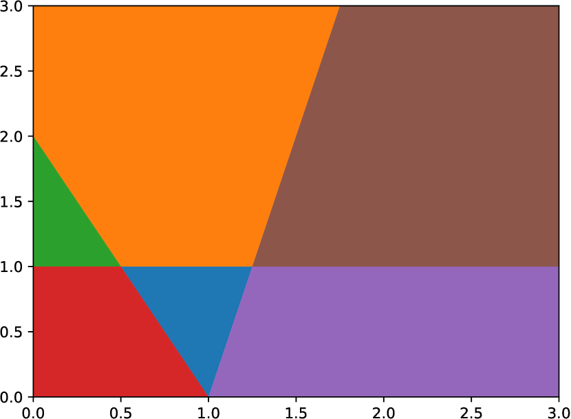
(a) Linear partitions in $\widehat{{f}_{\restriction X}}$ for the network

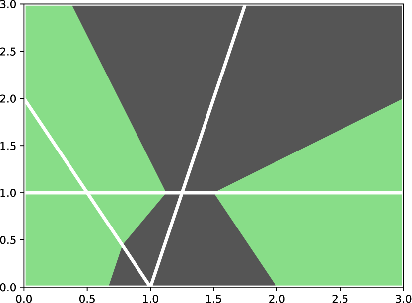
(b) Classification regions of the network

Figure 2. Symbolic representation of neural network $N_{1}$ defined by function $f$ in Equation 1

2.4. Understanding Network Behavior using Weakest Precondition

A first natural question to ask about a neural network is what inputs result in a particular set of outputs?Answering such questions corresponds to computing the weakest precondition, i.e. all points in $X$ that are mapped to $Y$ by ${f}_{\restriction X}$: $\textsc{WPre}({f}_{\restriction X},Y)=\{x\in X\mid f(x)\in Y\}$. Section 5.3 shows how $\widehat{{f}_{\restriction X}}$ can be used to efficiently compute this set, which may in general be non-convex.

For example, in our running scenario, we may wish to ask: which areas does the network $N_{1}$ predict will be habitable? The polytope $H=\{y\mid y_{2}>y_{1}\}$ denotes the set of output points that are habitable, similarly $U$ for uninhabitable points. Using $\widehat{{f}_{\restriction X}}$ (Figure 2(a)), we can compute $\textsc{WPre}({f}_{\restriction X},H)$ and $\textsc{WPre}({f}_{\restriction X},U)$, which represent the set of all habitable and uninhabitable points in $X$, respectively. Figure 2(b) plots these precondition sets on a two-dimensional axis with each set assigned a different color. Thus, we can precisely and exactly visualize the decision boundaries of a deep neural network using $\textsc{WPre}({f}_{\restriction X},Y)$.

Effectively, within each linear partition in Figure 2(b) (delineated with white borders), the network’s output is affine, and thus the decision boundary is linear — notice that the decision boundary is a single straight line in any given linear partition in Figure 2(b), even though the overall decision boundaries have “corners.” This allows us to quickly and precisely determine decision boundaries within each linear partition using standard linear algebra techniques (Section 5.3). An evaluation of $\textsc{WPre}({f}_{\restriction X},Y)$ on a large network is presented in Section 8.1, where we produce figures like Figure 3(a) that show how the advisory made by an aircraft collision-avoidance network depends on the location of an intruder.

2.5. Bounded Model Checking of Safety Properties using Strongest Postcondition

Consider another neural network, which controls a motor attached to an inverted pendulum which is in turn described by its current position $\theta$ and angular velocity $\omega$. The network takes $\theta$ and $\omega$ as inputs, and produces as output the angular acceleration to apply to the pendulum by the motor. The network is trained to keep the pendulum inverted, but it has not been formally verified that the network correctly accomplishes this goal for all valid starting conditions.

In Section 6, we address the problem of bounded model checking for such control networks. In particular, we show how the symbolic representation enables us to compute the strongest postcondition, i.e. the set of all possible outputs given that the input is in a particular region: $\textsc{SPost}(f,X)=\{f(x)\mid x\in X\}$. Consequently, we show how to verify the following claim for the inverted pendulum controller: Starting from any valid initial condition and applying the network controller to the system for $K$ time-steps, there is no timestep for which the pendulum becomes non-inverted (i.e., dips below the horizontal).

In Section 8.2, we evaluate our approach against one using ReluPlex (Katz et al., 2017) on the pendulum model and two other standard neural network controller models from Zhu et al. (2019).

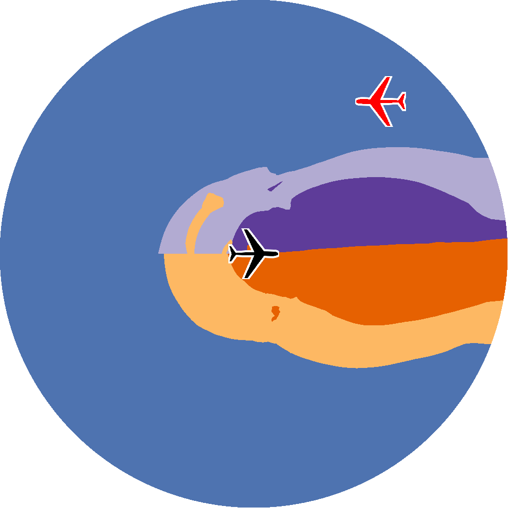
(a) Network visualization.

(b) Patched network visualization (plane icons removed to better show decision boundaries).

Figure 3. Visualizing preconditions for and patching an aircraft collision avoidance network.

Legend:   Clear-of-Conflict,   Weak Right,   Strong Right,   Strong Left,   Weak Left.

2.6. Patching Deep Neural Networks

Finally, we introduce the problem of patching a neural network. Patching a network $N$ entails fixing the behavior of $N$ in a particular region $R$ of the input space by modifying the weights of $N$. For example, in Figure 3(a), we see a visualization of the actions suggested by an aircraft collision avoidance system when an intruder is at different places relative to the ownship. For the most part, the network’s outputs seem reasonable; when the intruder is reasonably far away, it reports that the plane is “clear of conflict” (blue), when the intruder is nearby but on the left of the plane it instructs to make a “hard right” (dark purple), etc. However, we can also see that there are a number of regions in the input space where the network seems to make unsafe suggestions, eg. when the intruder is behind-and-to-the-left of the plane, we see a “band” of light orange that indicates the network has instructed a “weak left turn,” which would actually turn the ownship towards the intruder. We may want to patch this behavior, i.e. modify the weights of the network such that the network instead instructs “weak right,” which would turn the plane away from the intruder. A patch specification describes which regions of the input space we want to change the classification over and which we want the classification to stay the same.

With this patch specification in hand, we can formulate the problem as a MAX-SMT instance that can, in theory, be solved with an SMT solver such as Z3 (de Moura and Bjørner, 2008). However, the inherently non-linear and high-dimensional nature of our networks makes this infeasible. To remedy this, we transform the network into an equivalent Masking Network, described in Section 7.2. Then, we show in Theorem 3 how to use $\widehat{f}$ to translate this patch specification into a set of (finitely many) key points in the input space, for which patching on the key points is equivalent to patching on the regions. This allows us to lower the problem of patching on infinite regions to patching on finitely-many points, similar to how the simplex algorithm lowers optimization on polytopes to optimization on vertices. If we utilize these key points and restrict the number of weights we change at any one iteration, we show how to translate the previously-non-linear MAX-SMT instance into a linear one. Finally, we discuss a greedy MAX-SMT solver that can quickly find updates to individual weights that will maximize the number of key points with the correct classification. The result of this process is shown in Figure 3(b), where after changing only five weights the offending region has been removed.

In Section 8.3, we perform this process for the ACAS Xu network for a variety of different patch specifications, finding that it is able to effectively patch network behavior and that behavior patched in one region of the input space generalizes well to other regions.

3. A Symbolic Representation for Deep Neural Networks

In this section, we will introduce our symbolic function representation and discuss a number of immediate theoretical results relating to its definition.

In all below discussion, we will use the term “polytope” or “(bounded) polytope” to refer to the convex hull of finitely many points while we will use “(potentially unbounded) polytope” to refer to the intersection of finitely many half-spaces.

Given a function $f:A\to B$ where $A\subseteq\mathbb{R}^{a},B\subseteq\mathbb{R}^{b}$, we represent our symbolic representation $\widehat{f}$ as a set $\widehat{f}=\{(P_{1},F_{1}),(P_{2},F_{2}),\ldots,(P_{n},F_{n})\}$, where:

1. The set $\{P_{1},P_{2},\ldots,P_{n}\}$ should have each $P_{i}\subseteq A$ and, further, should partition $A$ (the domain of $f$), except possibly for overlapping boundaries.

2. Given any such $(P_{i},F_{i})$ pair, with $F_{i}:P_{i}\to B$, the following holds: $\forall x\in P_{i}:f(x)=F_{i}(x)$.

These two requirements describe a symbolic representation of $f$ by breaking its input into regions $P_{i}$ where the behavior of $f$ is captured by a (possibly simpler) function $F_{i}$.

However, as described, there is no reason to believe that the constituent $F_{i}$s will be more analysis-friendly than the original function $f$; indeed, $\widehat{f}=\{(A,f)\}$ meets the constraints listed above but clearly gives us no additional insight into $f$.

To remedy this, we further restrict our description to a form which noticeably improves our ability to analyze $f$:

1. Each $P_{i}$ is a convex polytope.

2. Each $F_{i}:P_{i}\to B$ is affine.

Indeed, the first condition ensures that the partitioning is efficiently representable and manipulatable, while the second condition ensures that we can use standard linear algebra techniques and algorithms to perform the desired analysis within any given partition.

Definition 1.

Given a function $f:A\to B$ where $A\subseteq\mathbb{R}^{a}$ and $B\subseteq\mathbb{R}^{b}$, we define the symbolic representation of $f$, written $\widehat{f}$, to be a set of tuples $\widehat{f}=\{(P_{1},F_{1}),\ldots,(P_{n},F_{n})\}$, such that:

1. The set $\{P_{1},P_{2},\ldots,P_{n}\}$ partitions the domain of $f$, except possibly for overlapping boundaries.

2. Given any such $(P_{i},F_{i})$ pair, the following holds: $\forall x\in P_{i}:f(x)=F_{i}(x)$.

3. Each $P_{i}$ is a convex polytope.

4. Each $F_{i}:P_{i}\to B$ is affine.

As discussed in Section 2.2, we can often improve the efficiency of the symbolic representation by only computing it over the restricted domain $X$, which we call the symbolic representation of $f$ restricted to $X$ and write $\widehat{{f}_{\restriction X}}$. Notably, Definition 1 still holds; we have simply explicitly stated that the domain $A$ is the set we have defined as $X$. Thus, in definitions we will usually only use the explicit syntax $\widehat{{f}_{\restriction X}}$ when we wish to place restrictions on the possible values of the domain $X$ (for example, to state that an algorithm only works when the domain is bounded).

Finally, we define another primitive, denoted by the operator $\otimes$ and sometimes referred to as Extend, such that $\textsc{Extend}{}(h,\widehat{g})=h\otimes\widehat{g}=\widehat{h\circ g}$. This is the primitive which we will implement in our algorithms, as it enables easy composition across multiple layers in a neural network. For example, suppose one wishes to compute $\widehat{{f}_{\restriction X}}$ where $f=f_{n}\circ f_{n-1}\circ\cdots\circ f_{1}$, and has access to algorithms for computing $\textsc{Extend}{}(f_{i},\cdot)$ for each composed function $f_{i}$.

Then, we can initially define the identity map $I:x\mapsto x$, which is affine across its entire input space, so we always have $\widehat{{I}_{\restriction X}}=\{(X,I)\}$ Then, by the definition of $\textsc{Extend}{}(f_{1},\cdot)$, we can compute: $f_{1}\otimes\widehat{{I}_{\restriction X}}=\widehat{{(f_{1}\circ I)}_{\restriction X}}=\widehat{{f_{1}}_{\restriction X}}$ (The final equality holds as, by the definition of the identity map $I$, $g\circ I=g$ holds for any function $g$.)

We can then iteratively apply this procedure to inductively compute $\widehat{{(f_{i}\circ f_{i-1}\circ\cdots f_{1})}_{\restriction X}}$ from $\widehat{{(f_{i-1}\circ\cdots f_{1})}_{\restriction X}}$ like so: $f_{i}\otimes\widehat{{(f_{i-1}\circ\cdots\circ f_{1})}_{\restriction X}}=\widehat{{(f_{i}\circ f_{i-1}\circ\cdots\circ f_{1})}_{\restriction X}}$ until we have computed $\widehat{{(f_{n}\circ f_{n-1}\circ\cdots\circ f_{1})}_{\restriction X}}=\widehat{{f}_{\restriction X}}$.

A number of properties follow immediately from these definitions, which we summarize here and prove in full in Appendices A—F. First, we find a number of negative results, describing functions (or classes of functions) for which $\widehat{f}$ and $\widehat{{f}_{\restriction X}}$ cannot be computed.

Theorem 2.

There exists a continuous, fully-differentiable function $f$ such that $\widehat{f}$ does not exist.

Theorem 3.

There exists a continuous, fully-differentiable function $f$ such that $\widehat{{f}_{\restriction X}}$ does not exist for any non-singleton and non-empty choice of $X$.

Both of these theorems can be understood by considering the function $f(x)=x^{2}$. The key insight is that $f$ behaves non-linearly on its entire input domain; there are no two $x_{1}<x_{2}$ such that $f(x+x^{\prime})=f(x)+f(x^{\prime})$ and $f(cx)=cf(x)$ for all $x_{1}\leq x,x^{\prime}\leq x_{2}$. However, as the next theorem shows, sometimes restricting the function to a particular input domain can make the symbolic representation computable.

Theorem 4.

There exists a continuous, fully-differentiable function $f$ and a non-singleton, non-empty polytope $X$ such that $\widehat{f}$ does not exist but $\widehat{{f}_{\restriction X}}$ does.

An example for this theorem can be seen in the function $f(x_{1},x_{2})=\sin^{2}{x_{1}}+\cos^{2}{x_{2}}$, which in general behaves non-linearly, but when restricted to input points where $x_{1}=x_{2}$, it satisfies the affine relation $f(x_{1},x_{2})=1$. A similar example is the function $f(x_{1},x_{2})=(x_{1}+x_{2})(x_{1}-x_{2})$, which is non-linear except when $x_{1}-x_{2}$ equals a constant.

Next, we have a number of positive results, showing that $\otimes$ both exists and is computable for functions that are commonly composed to create neural networks.

Theorem 5.

For any piecewise-linear function $f$, $f\otimes\widehat{g}$ is computable for any $\widehat{g}$.

Corollary 0.

$\textsc{FullyConnected}{}\otimes\widehat{g}$ is computable for any $\widehat{g}$.

Corollary 0.

$\textsc{2DConvolution}{}\otimes\widehat{g}$ is computable for any $\widehat{g}$.

Corollary 0.

$\textsc{BatchNorm}{}\otimes\widehat{g}$ is computable for any $\widehat{g}$.

Corollary 0.

$\textsc{ReLU}{}\otimes\widehat{g}$ is computable for any $\widehat{g}$.

Corollary 0.

$\textsc{MaxPool}{}\otimes\widehat{g}$ is computable for any $\widehat{g}$.

Corollary 0.

$f\otimes\widehat{g}$ is computable for any $\widehat{g}$ and neural network $f$ consisting of sequentially-applied FullyConnected, 2DConvolution, BatchNorm, ReLU, and MaxPool layers.

4. Algorithms for Computing $\widehat{{f}_{\restriction X}}$

In this section, we discuss algorithms for computing $\widehat{{f}_{\restriction X}}$ for piecewise-linear functions (see Definition 1). Recall the primitive Extend, where $\textsc{Extend}{}(h,\widehat{g})=h\otimes\widehat{g}=\widehat{h\circ g}$. We showed in Section 3 that, as long as you can compute Extend for each layer type in a network, you can compute $\widehat{f}$ for the entire network. Thus, we focus in this section on algorithms for computing Extend for common neural network layers.

In Section 4.1 we define a number of standard functions that we will use in the algorithms. In Section 4.2, we describe the rectified linear unit, a common piecewise-linear function used in deep neural networks. In Section 4.3, we present an efficient algorithm for the case when the restriction domain of interest is two-dimensional. In Section 4.4 we generalize the ReLU algorithm to arbitrary piecewise-linear functions with two-dimensional restriction domain of interest. Finally, in Section 4.5, we discuss the benefits of the polytope representation used by our algorithm.

4.1. Definitions and Common Functions

Here we define a number of functions which we will use in our algorithms:

1. Given a (bounded) polytope $X$, Vert($X$) returns a list of its vertices in counter-clockwise order, repeating the initial vertex at the end.

2. Given a set of points, ConvexHull($X$) computes their convex hull (i.e., smallest bounded polytope containing all points in $X$).

3. Given a scalar value $x$, Sign($x$) computes the sign of that value (i.e., $-1$ if $x<0$, $+1$ if $x>0$, and $0$ if $x=0$).

4. Given a polytope $X$ which must lie in a single orthant, OrthantSign($X$) computes the per-coefficient sign corresponding to that orthant.

   For example, if $X=\textnormal{{ConvexHull}}(\{(1,-1),(2,-3),(4,-2)\})$, then OrthantSign($X$) $=(1,-1)$.

5. Given a polytope $X$ and affine map $A$, $A^{\#}(X)$ represents the polytope formed by applying $A$ to every point in $X$.

4.2. A case study in PWL Functions: The Rectified Linear Unit

The Rectified Linear Unit function, ReLU, is one of the standard neural network non-linearities used today. Recall from Section 2.1 that it can be defined as a piecewise-linear function taking in vector $x=(x_{1},x_{2},\ldots,x_{n})$ and computing $\textsc{ReLU}{}(x)=(\textsc{ReLU}{}(x)_{1},\ldots,\textsc{ReLU}{}(x)_{n})$ where:

$$\textsc{ReLU}{}(x)_{i}=\begin{cases}0&x_{i}\leq 0\\ x_{i}&x_{i}>0\end{cases}$$

Geometrically, the ReLU function can be thought of as projecting points onto the faces of the positive orthant by zeroing-out negative coefficients. Notably, if a set of points all lie in the same orthant (i.e., all have the same sign), then applying ReLU to all of them corresponds to applying a single affine projection to all of them (namely, the identity map with non-positive entries on the diagonal zeroed out). Thus, intuitively the computation can be broken down into multiple affine projections, one for the portion of the polytope in each orthant.

4.3. Input-Aware, Rectified Linear Units in Two Dimensions

We now present an efficient algorithm for computing $\textsc{ReLU}{}\otimes\widehat{g}$ when $\widehat{g}$ involves only bounded, two-dimensional polytopes. This algorithm strives to display both efficient best- and worst-case execution time. The key insight is that, when a polytope is all in a single orthant, the application of ReLU is an affine function. We read each polytope as a counter-clockwise set of vertices, following around the edges between vertices until the edge of the polytope intersects an orthant boundary. At that point, we split the polytope in two, such that each half lies on only one side of the orthant boundary. Repeating this process recursively ensures that the resulting polytopes lie on only one side of all orthant boundaries, i.e. each lies completely in a single orthant.

Input: $V$, the vertices of the polytope in the input space of $g$. $F$, the affine map that corresponds to $g$ within $\textnormal{{ConvexHull}}(V)$. $i$ is the index of the last vertex lying on the same side of the orthant face as $V_{1}$. $j$ is the index of the last vertex lying on the opposite side of the orthant face as $V_{1}$. $d$ is the index of the orthant face, i.e. the face is $x_{d}=0$.

Output: $\{P_{1},P_{2}\}$, two sets of vertices whose convex hulls form a partitioning of $V$ such that each lies on only one side of the $x_{d}=0$ hyperplane.

1 $p_{i}\leftarrow V_{i}-\frac{F(V_{i})_{d}}{F(V_{i+1})_{d}-F(V_{i})_{d}}(V_{i+1}-V_{i})$

2 $p_{j}\leftarrow V_{j}-\frac{F(V_{j})_{d}}{F(V_{j+1})_{d}-F(V_{j})_{d}}(V_{j+1}-V_{j})$

3 $A\leftarrow\{p_{i},p_{j}\}\cup\{v\in V\mid\textnormal{{Sign}}(v_{d})=\textnormal{{Sign}}({V_{i}}_{d})\}$

4 $B\leftarrow\{p_{i},p_{j}\}\cup\{v\in V\mid\textnormal{{Sign}}(v_{d})=\textnormal{{Sign}}({V_{j}}_{d})\}$

return $\{A,B\}$

Algorithm 1 SplitPlane$(V,F,i,j,d)$

Input: $\widehat{g}=\{(P_{1},F_{1}),\ldots,(P_{n},F_{n})\}$.

Output: $\widehat{{\textsc{ReLU}{}\circ g}_{\restriction X}}$

1 $W\leftarrow$ ConstructQueue($\widehat{{g}_{\restriction X}}$)

2 $Y\leftarrow\emptyset$

3 while $W$ not empty do

4       $P,F\leftarrow$ Pop($W$)

5       $V\leftarrow\textnormal{{Vert(}}\textnormal{\emph{$P$}}\textnormal{{)}}$

6       $K\leftarrow\{k\mid\exists i,j:\textnormal{{Sign}}(F(V_{i})_{k})>0\wedge\textnormal{{Sign}}(F(V_{j})_{k})<0\}$

7       if $K=\emptyset$ then

8             $Y\leftarrow Y\cup\{(P,\textsc{ReLU}{}[\textnormal{{OrthantSign}}(F^{\#}(P))]\circ F)\}$

9             continue

10      $k\leftarrow$ any element from $K$

11       $i\leftarrow\operatorname*{arg\,max}_{i}\{\textnormal{{Sign}}(F(V_{i})_{d})=\textnormal{{Sign}}(F(V_{1})_{d})\}$

12       $j\leftarrow\operatorname*{arg\,max}_{j}\{\textnormal{{Sign}}(F(V_{j})_{d})\neq\textnormal{{Sign}}(F(V_{i})_{d})\}$

13       for $V^{\prime}\in\textnormal{{SplitPlane}}(V,F,i,j,d)$ do

14             $W\leftarrow$ Push($W,(\textnormal{{ConvexHull}}(V^{\prime}),F)$)

15            

16      

return $Y$

Algorithm 2 $\textsc{ReLU}{}\otimes\widehat{g}$ for two-dimensional $\widehat{g}$ partitions.

Notably, in the best-case scenario where each partition is in a single orthant, the algorithm never calls SplitPlane() at all — it simply iterates over all of the $n$ input partitions, checks their $v$ vertices, and appends to the resulting set (for a best-case complexity of $O(nv)$). In the worst case, it splits each polytope in the queue on each face, resulting in exponential time complexity. In practice, however, we find that this algorithm is very efficient and can be applied to real-world networks effectively (see Section 8).

The proofs of the following theorems can be found in Appendices G—H:

Theorem 1.

Algorithm 1 correctly splits a 2D polytope $\textnormal{{ConvexHull}}(V)$ by the hyperplane $x_{d}=0$.

Theorem 2.

Algorithm 2 correctly computes $\widehat{{\textsc{ReLU}{}\circ g}_{\restriction X}}$.

4.4. Arbitrary Piecewise-Linear Function in Two Dimensions

We can generalize Algorithm 2 to arbitrary piecewise-linear functions $f$. We let the domain of $f$ be partitioned by a finite number of polytopes stored in H-representation (i.e., as a conjunction of half-spaces). We then take the set of all hyperplanes defining the partitioning polytopes, defined by affine maps $\{A_{1},A_{2},\ldots,A_{m}\}$. The insight is now essentially the same: subdividing the input polytope such that each sub-divided polytope lies entirely on one side of each hyperplane $A_{i}$ ensures that it lies entirely within a particular linear region of $f$. Effectively, the only difference between these algorithms and those specialized to ReLU is that we replace the particular affine map $v_{d}$ (i.e., projection onto the $d$ dimension) with ones specified by the function $f$ from the set of $A_{i}$s.

4.5. Representing Polytopes

Finally, we close this section with a discussion of implementation concerns when representing the convex polytopes that make up the partitioning of $\widehat{{f}_{\restriction X}}$. In standard computational geometry, bounded polytopes can be represented in two equivalent forms:

1. The half-space or H-representation, which encodes the polytope as an intersection of finitely-many half-spaces. (Each half-space being defined as one side of a hyperplane, which can in turn be defined by an affine map $Ax\leq 0$.)

2. The vertex or V-representation, which encodes the polytope as a set of finitely many points; the polytope is then taken to be the convex hull of the points (i.e., smallest convex shape containing all of the points.)

However, choosing a particular representation can make certain problems significantly easier or more challenging. Finding the intersection of two polytopes in an H-representation, for example, can be done in linear time by simply concatenating their representative half-spaces, but the same is not possible in V-representation.

In our algorithms, there are two main operations we need to do with polytopes in our algorithms: splitting a polytope with a hyperplane and applying an affine map to all points in the polytope. In general, the first is more efficient in an H-representation, while the latter is more efficient in a V-representation. However, when restricted to two-dimensional polygons, the former is also efficient in a V-representation, as demonstrated by Algorithm 1, helping to motivate our use of the V-representation in our algorithms.

Furthermore, the representations differ as to their resiliency to floating-point operations. In particular, H-representations for polytopes in $\mathbb{R}^{n}$ are notoriously difficult to achieve high-precision with, as the error introduced from using floating point numbers gets arbitrarily large as one goes in a particular direction along any hyperplane face. Ideally, we would like the hyperplane to be most accurate in the region of the polytope itself, which corresponds to choosing the magnitude of the norm vector correctly. Unfortunately, to our knowledge, there is no efficient algorithm for computing the ideal floating point H-representation of a polytope, although libraries such as APRON (Jeannet and Miné, 2009) are able to provide reasonable results for low-dimensional spaces. However, as neural networks utilize extremely high-dimensional spaces (i.e., thousands of dimensions) and we wish to iteratively apply our analysis, we find that errors from using floating-point H-representations can quickly multiply and compound to become infeasible. By contrast, floating-point inaccuracies in a V-representation are directly interpretable as slightly misplacing the vertices of the polytope; no “localization” process is necessary to penalize inaccuracies close to the polytope more than those far away from it.

Another difference is in the space complexity of the representation. In general, H-representations can be more space-efficient for common shapes than V-representations, however, when the polytope lies in a low-dimensional subspace of a larger space, the V-representation is usually significantly more efficient.

Thus, V-representations are a good choice for low-dimensionality polytopes embedded in high-dimensional space, which is exactly what we need for analyzing neural networks with two-dimensional restriction domains of interest. This is why we designed our algorithms to rely on $\textnormal{{Vert}}(X)$, so that they could be directly computed on a V-representation.

5. Understanding network behavior using weakest precondition

In this section, we investigate one of the most immediate questions one might ask when analyzing a neural network: what inputs lead to a particular set of outputs?

5.1. The $\textsc{Pre}({f}_{\restriction X},Y)$ Primitive

5.1.1. Preconditions

This problem is formalized by the notion of preconditions; subsets of the input space which, when $f$ is applied, map to a particular set of outputs. We now introduce a primitive that describes the notion of such preconditions for a neural network $f:A\to B$ and output polytope $Y\subseteq B$: $\textsc{Pre}({f}_{\restriction X},Y)\subseteq\{x\in X\mid f(x)\in Y\}$. $\textsc{Pre}({f}_{\restriction X},Y)$ always satisfies the following properties:

1. $\textsc{Pre}({f}_{\restriction X},Y)\subseteq X$

2. For any $x\in\textsc{Pre}({f}_{\restriction X},Y)$, $f(x)\in Y$ holds.

5.1.2. Weakest Precondition

The definition of $\textsc{Pre}({f}_{\restriction X},Y)$ only requires an under approximation; there may be points $x\in X$ such that $f(x)\in Y$, even if $x\not\in\textsc{Pre}({f}_{\restriction X},Y)$. This leads to the fact that $\emptyset$, which we refer to as the strongest precondition, always satisfies $\textsc{Pre}({f}_{\restriction X},Y)=\emptyset$. However, such a solution is not particularly useful, and instead we would like to find the weakest precondition $\textsc{WPre}({f}_{\restriction X},Y)=\{x\in X\mid f(x)\in Y\}$.

For arbitrary functions and regions, $\textsc{WPre}({f}_{\restriction X},Y)$ may not be convex or even representable as a union of convex shapes. However, we will show by construction in Section 5.3 that, when $\widehat{{f}_{\restriction X}}$ exists and $Y$ is a convex polytope, $\textsc{WPre}({f}_{\restriction X},Y)$ can be represented precisely as a union of finitely many convex polytopes.

5.2. DPPre: Computing Preconditions with DeepPoly

We first investigate one way in which a solution to $\textsc{Pre}({f}_{\restriction X},Y)$ can be found using prior work in abstract interpretation. DeepPoly (Singh et al., 2019) is an abstract representation of the neural network ${f}_{\restriction X}$ included as part of the ERAN abstract interpretation package (ERA, 2019). Namely, for any network $f$ restricted to restriction domain of interest $X$ (i.e., ${f}_{\restriction X}$) and any particular output dimension $i$, DeepPoly can produce lower- and upper-bound affine maps $A_{i}^{l}$ and $A_{i}^{u}$ such that, for all $x\in X$: $A_{i}^{l}x\leq{f_{i}}_{\restriction X}(x)\leq A_{i}^{u}x$. Thus, as long as the set $Y$ is convex, it follows that $\{x\in X\mid A_{i}^{l}x\in Y\wedge A_{i}^{u}x\in Y\}$ is a valid $\textsc{Pre}({f}_{\restriction X},Y)$. This set can be computed explicitly from $A_{i}^{l}$ and $A_{i}^{u}$ using a variety of linear algebra techniques, and a geometric interpretation of this process is discussed below.

One can think of the DeepPoly representation as defining two polytopes, each one a two-vocabulary polytope in a space consisting of both input and output dimensions of the network. The first polytope defines the lower bounds on the network output: $D_{l}=\{(x,y)\mid x\in X\wedge y=A^{l}(x)\}$ and the second defines the upper bounds on the network output: $D_{u}=\{(x,y)\mid x\in X\wedge y=A^{u}(x)\}$, where $A^{l}(x)=(A^{l}_{1}(x),\ldots,A^{l}_{n}(x))$, i.e. lower bounds for all output dimensions (and similar for $A^{u}(x)$). Computing $\textsc{Pre}({f}_{\restriction X},Y)$ can now be seen as a three step process:

1. Compute the intersection of $D_{l}$ with $Y$ and project onto only the input $x$ dimensions, resulting in a new polytope $P_{l}$. $P_{l}$ contains only input points for which we can guarantee the image under $f$ is lower-bounded by some value within $Y$.

2. Compute the intersection of $D_{u}$ with $Y$ and project onto only the input $x$ dimensions, resulting in a new polytope $P_{u}$. $P_{u}$ contains only input points for which we can guarantee the image under $f$ is upper-bounded by some value within $Y$.

3. Compute the intersection of $P_{l}$ and $P_{u}$, representing inputs which have lower and upper bounds in $Y$, thus (by convexity) the actual output must lie in $Y$.

We refer to this approach as $\operatorname*{DPPre}$ or $\operatorname*{DPPre}[1]$. Notably, this intersection-projection construction implies that $\textsc{Pre}({f}_{\restriction X},Y)$ found using DPPre can only represent convex shapes, thus it in general cannot find $\textsc{WPre}({f}_{\restriction X},Y)$ which may be non-convex. This is usually fine for local-behavior verification problems where the network acts mostly convex, but is in practice unsuited for computing precise $\textsc{Pre}({f}_{\restriction X},Y)$ sets when $\textsc{WPre}({f}_{\restriction X},Y)$ is highly non-convex. In practice, the precision of $\textsc{Pre}({f}_{\restriction X},Y)$ computed with DeepPoly can be improved by pre-partitioning the input space $X$ into smaller regions and passing each region to the analyzer separately. We notate this approach as DPPre[k], defined by:

Definition 1.

Suppose $X$ is a bounded restriction domain of interest spanned by $d$ basis vectors. Then DPPre[k](${f}_{\restriction X},Y$) is the application of the DPPre process after evenly splitting $X$ in each of the $d$ basis directions into $k$ equal partitions.

$$\operatorname*{DPPre}[k]({f}_{\restriction X},Y)\buildrel\mbox{\tiny{def}}\over{=}\bigcup_{i_{1}=1}^{k}\bigcup_{i_{2}=1}^{k}\cdots\bigcup_{i_{d}=1}^{k}\operatorname*{DPPre}[1]({f}_{\restriction Part(X,k,i_{1},i_{2},\ldots,i_{d})},Y)$$

Where $Part(X,k,i_{1},\cdots,i_{d})$ is the $(i_{1},\cdots,i_{d})$th partition of $X$ when $X$ is split by $k$ equal partitions along each basis. For example, if $X=\{(x,y)\mid 0\leq x\leq 1\wedge 0\leq y\leq 1\}$ and we use the standard basis $\{(1,0),(0,1)\}$, then $Part(X,4,1,1)=\{(x,y)\mid 0\leq x\leq\frac{1}{4}\wedge 0\leq y\leq\frac{1}{4}\}$.

As we will see in Section 8.1, even when using $k$ as large as $100$ (i.e., $10,000$ partitions for a two-dimensional region) the precision is still lacking. Furthermore, performance suffers as the number of DPPre[1] calls grows according to $k^{d}$.

5.3. Computing Weakest Preconditions with $\widehat{{f}_{\restriction X}}$

The exact $\textsc{WPre}({f}_{\restriction X},Y)$ can be computed given $\widehat{{f}_{\restriction X}}=\{(P_{1},F_{1}),\ldots,(P_{n},F_{n})\}$. Effectively, within each $(P_{i},F_{i})$ and for all $x\in P_{i}$ and output dimension $j$, we have: ${f}_{\restriction X}(x)_{j}=(F_{i}x)_{j}$, which is similar to the form returned by DeepPoly except the bounds are exact — there is no over-approximation at all. Then, we can intersect the corresponding polytopes to compute $\textsc{WPre}({{F_{i}}}_{\restriction{P_{i}}},Y)$ on each $(P_{i},F_{i})$ pair; the union of all such regions is then $\textsc{WPre}({f}_{\restriction X},Y)$.

5.4. Visualizing Decision Boundaries with $\textsc{Pre}({f}_{\restriction X},Y)$

Many neural networks are classifiers, meaning they take some input and produce one of a small (finite) set of outputs. An example of such a network is the ACAS Xu aircraft avoidance network (Julian et al., 2018), which has five inputs describing the position and velocity of an “ownship” and “intruder,” transformed through five “hidden layers” with 50 dimensions each, then produces five real-valued outputs $y_{1},\ldots,y_{5}$. The network’s output space is to be interpreted as having five classification regions, partitioning the output space depending on which output dimension is maximal. For example, the network may be said to advise a “strong right” turn when $f(x)\in R_{5}$, with $R_{5}$ (“the fifth classification region”) defined as $R_{5}=\{y\mid y_{5}>y_{1}\wedge\cdots\wedge y_{5}>y_{4}\}$.

Suppose we want to visualize the policy learned by the network. We could fix all inputs (eg. the velocity and heading) other than the position of the attacking ship, resulting in a restriction domain of interest denoted $X$. Then, we could compute $\textsc{WPre}({f}_{\restriction X},R_{5})$ to get the set of all such input positions for which the network advises to make a “strong right,” and use standard computer graphics tools to plot these points on a graph in a particular color (say, orange). We may then repeat the process, until we have plotted $\textsc{WPre}({f}_{\restriction X},R_{1})$ through $\textsc{WPre}({f}_{\restriction X},R_{5})$ on the same plot in separate colors. The process is shown in Section 8.1, and the resulting plot can provide precise and immediate insight into the behavior of an ownship controlled by the network.

6. Bounded model checking of safety properties using strongest postcondition

We saw in the preceding section how $\widehat{{f}_{\restriction X}}$ can be used to compute the weakest precondition of a network’s input given conditions on the output, then described how that primitive could be applied to visualizing decision boundaries of a neural network. In this section, we consider a complementary primitive called the strongest postcondition, and show how it can be used to perform bounded model checking (Biere et al., 2009) of neural-network based controllers.

6.1. The $\textsc{Post}(f,X)$ Primitive

We define $\textsc{Post}(f,X)$ to be a set containing all output points that can be mapped to under $f$ given some input in $X$. Formally, for a neural network $f:A\to B$ and input polytope $X\subseteq A$, we have $\{f(x)\mid x\in X\}\subseteq\textsc{Post}(f,X)\subseteq B$. $\textsc{Post}(f,X)$ always satisfies the following properties:

1. $\textsc{Post}(f,X)\subseteq B$

2. For any $x\in X$, $f(x)\in\textsc{Post}(f,X)$.

6.1.1. Strongest Postcondition

Notably, this definition only requires an over approximation; there may be points $y\in\textsc{Post}(f,X)$ such that there is not any $x\in X$ satisfying $f(x)=y$. This leads to the fact that $B$ (the range of $f$), which we refer to as the weakest postcondition, always satisfies $\textsc{Post}(f,X)=B$. However, such a solution is not particularly useful, and instead in general we would like to find the strongest postcondition, denoted $\textsc{SPost}(f,X)$, which exactly satisfies $\textsc{SPost}(f,X)=\{f(x)\mid x\in X\}$.

For arbitrary functions and regions, $\textsc{SPost}(f,X)$ may not be convex or even representable as a union of convex shapes. However, we will show by construction in Section 6.2 that, when $\widehat{{f}_{\restriction X}}$ exists and $X$ is a convex polytope, $\textsc{SPost}(f,X)$ can be represented precisely as a union of finitely many convex polytopes.

6.2. Computing $\textsc{SPost}(f,X)$ with $\widehat{{f}_{\restriction X}}$

Suppose we wish to compute $\textsc{SPost}(f,X)$, and know that $\widehat{{f}_{\restriction X}}=\{(P_{1},F_{1}),$ $\ldots,$ $(P_{n},F_{n})\}$. We first note that $\textsc{SPost}(f,X)=\bigcup_{(P_{i},F_{i})\in\widehat{{f}_{\restriction X}}}\textsc{SPost}(f,P_{i})=\bigcup_{(P_{i},F_{i})\in\widehat{{f}_{\restriction X}}}\textsc{SPost}(F_{i},P_{i})$. The first equality holds because the $P_{i}$s partition $X$ and the second equality holds because, given any $x\in P_{i}$, $f(x)=F_{i}(x)$.

Thus, it suffices to compute $\textsc{SPost}(F,P)$ for a polytope $P$ and affine function $F$. We note that, in computational geometry field, this corresponds to transforming polytope $P$ under affine map $F$, which in turn can be shown to correspond to transforming the vertices of $P$ and then taking the convex hull of the resulting vertices (due to the convexity of $P$ and $F$). In other words, we have $\textsc{SPost}(F,P)=\{F(x)\mid x\in P\}=\textnormal{{ConvexHull}}(\{F(v)\mid v\in\textnormal{{Vert}}(P)\})$, giving us, in total $\textsc{SPost}(f,X)=\bigcup_{(P_{i},F_{i})\in\widehat{{f}_{\restriction X}}}\textnormal{{ConvexHull}}(\{F_{i}(v)\mid v\in\textnormal{{Vert}}(P_{i})\})$.

6.3. Inverted Pendulum Model

In this section, we will consider a model taken from Zhu et al. (2019), which describes an inverted pendulum with a motor at the base which can apply angular acceleration to the pendulum. The motor is controlled by a neural network, which has been trained to keep the pendulum upright. The network takes as input two variables representing the state of the system, namely the current position of the pendulum and the current angular velocity. It then produces one output, namely the angular acceleration it wishes to apply. We call this network an actor and denote it $f$. Notably, we replaced $\tanh$ non-linearities with their piecewise-linear counterpart the hard tanh $g(x)=\mathrm{min}(\max(x,-1),1)$ (Collobert, 2004).

In the model used for training and verifying the network, the effect of applying a particular acceleration $a$ at time $t$ to state $x_{t}$ to form new state $x_{t+1}$ is modeled with an affine function that takes as input the previous state $x_{t}$ and the action $a$ and produces a new state $x_{t+1}$. We call this function an environment model and denote it $E$.

We can compose $E$ with $f$ to produce a new “transition function” $T(x_{t})=E(x_{t},f(x_{t}))=x_{t+1}$, which accepts as input a state $x_{t}$ and produces as output the corresponding state of the system after applying the acceleration prescribed by the network for one timestep. Because $f$ is piecewise-linear and $E$ is affine, it follows that $T$ itself is piecewise-linear. With this notation, we are now ready to describe a correctness specification for the network.

Definition 1.

Given a function $f:A\to B$, we define a correctness specification $C$ to be a set of tuples $\{(X_{1},Y_{1}),\ldots,(X_{n},Y_{n})\}$ where each $X_{i}\subseteq A$ and each $Y_{i}\subseteq B$.

We say $f$ meets specification $C$ if, for all $(X_{i},Y_{i})$ pairs and all $x\in X_{i}$, $f(x)\in Y_{i}$ is satisfied.

In contrast, we say $f$ violates specification $C$ if there exists some $(X_{i},Y_{i})$ pair and some $x\in X_{i}$ such that $f(x)\not\in Y_{i}$.

In the pendulum example, we will consider three sets of states:

1. The set of initial states $S_{I}=\{(\nu,\omega)\mid-0.35\leq\nu\leq 0.35\wedge-0.35\leq\omega\leq 0.35\}$ is the set of states the pendulum can be in before applying the network.

2. The set of safe states $S_{S}=\{(\nu,\omega)\mid-0.5\leq\nu\leq 0.5\wedge-0.5\leq\omega\leq 0.5\}$ is the set of states for which we say the network has succeeded, namely when the pendulum is upright and not moving at an unsafe speed.

3. The set of unsafe states $S_{U}=\{(\nu,\omega)\mid(\nu,\omega)\not\in S_{S}\}$ is the set of states for which we say the network has failed, namely when the pendulum dips below the horizontal or moves at an unsafe speed.

We would now like to solve the following bounded model checking problem: Is there any initial state such that, after applying the neural controller for $K$ time steps, the pendulum has ever reached an unsafe state? This corresponds to verifying the specification:

(2) $$\big{\{}(S_{I},S_{S}),(\textsc{SPost}(T,S_{I}),S_{S}),(\textsc{SPost}(T,S_{I})^{2},S_{S}),\ldots,(\textsc{SPost}(T,S_{I})^{K-1},S_{S})\big{\}}$$

where $\textsc{SPost}(T,S_{I})^{n}$ indicates the repeated application of $\textsc{SPost}(T,\cdot)$; for instance, $\textsc{SPost}(T,S_{I})^{2}$ $=$ $\textsc{SPost}(T,\textsc{SPost}(T,S_{I}))$.

6.4. Bounded Model Checking with DeepPoly

One could attempt to use DeepPoly (Singh et al., 2019) here as well, however, as DeepPoly uses an over-approximation for $\textsc{Post}(f,x)$, we would expect to run into many false-positives (where DeepPoly reports that the specification cannot be verified, but is unable to state whether that is due to imprecision in the abstraction used or because the specification is violated).

6.5. Bounded Model Checking with ReluPlex

Another approach we could take is to use the DNN-oriented SMT solver ReluPlex (Katz et al., 2017). Because $T$ is piecewise-linear, ReluPlex can handle queries such as: $\exists x\in S_{I}:T(x)\in S_{U}$ (with the caveat that, as $S_{U}$ is non-convex, it will have to be partitioned into convex polytopes before ReluPlex can be queried). Notably, however, ReluPlex does not support universal quantifiers on iterated applications of $T$, i.e. there is no meaningful way of encoding $\forall k\in\{1,2,\ldots,K\}:\exists x\in S_{I}:T^{k}(x)\in S_{U}\}$, where $T^{k}(x)$ is the repeated application of $T$ to $x$ $k$ times, which is the actual query we wish to run. Instead, we need to query ReluPlex separately for each timestep, forcing it to repeat work done on verifying properties of the behavior of the network on earlier timesteps at each new timestep.

6.6. Bounded Model Checking with $\widehat{{f}_{\restriction X}}$ and $\textsc{SPost}(f,X)$

Alternatively, one can perform the bounded model checking iteratively using $\textsc{SPost}(T,X)$, computed as discussed in Section 6.2. This works as follows:

Initially, we compute $\textsc{SPost}(T,S_{I})$ and check if $\textsc{SPost}(T,S_{I})\cap S_{U}=\emptyset$. If the intersection is not empty, then by definition there must be some state in $S_{I}$ that transitions to an unsafe state (in $S_{U}$) after applying the network for one timestep and we can report that the model has violated the specification. Next, we can use the computed $\textsc{SPost}(T,S_{I})$ and compute $\textsc{SPost}(T,\textsc{SPost}(T,S_{I}))=\textsc{SPost}(T,S_{I})^{2}$, which we can then check to see if any intersection with $S_{U}$ is found. We can repeat this iteratively, effectively “growing” the “reachable set” of our model at each step. If, upon reaching $\textsc{SPost}(T,S_{I})^{K}$, no intersection with $S_{U}$ has ever been identified, we may safely say that the model satisfies the specification in Equation 2. Importantly, we can iteratively reuse the computation of $\textsc{SPost}(T,S_{I})^{j}$ for computing $\textsc{SPost}(T,S_{I})^{j+1}$, as opposed to the SMT-solver approach which does not share information between verification of different step lengths.

There are multiple further optimizations that can be performed in this approach. For example, $\widehat{{f}_{\restriction S_{S}}}$ can be computed and stored once ahead-of-time, so $\textsc{SPost}(T,S_{I})^{j}$ can be immediately computed without having to repetitively re-compute our symbolic representation of $f$. Furthermore, if something in one step has already been included in the post-set of a previous step, it can be safely ignored when propagating to the next step. For an extreme example, if $\textsc{SPost}(T,S_{I})\subseteq S_{I}$ (and $S_{I}\cap S_{U}=\emptyset$) we could immediately verify the network for all $K$ timesteps (in fact, all timesteps in general) because it satisfies the inductive invariant $\textsc{SPost}(T,S_{I})^{j}\subseteq S_{I}\wedge S_{I}\cap S_{U}=\emptyset$ for all $j$.

7. Patching Deep Neural Networks

Figure 4. Patching deep neural networks

In this section, we introduce and formalize the problem of network patching, then show how our symbolic representation of a DNN can lead to a solution to the network patching problem (Figure 4). As a running example, consider the expository neural network defined by function $f$ below:

(3) $$f(x)=\begin{bmatrix}1&1&1\\ 0&-1&-1\end{bmatrix}\textsc{ReLU}{}\left(\begin{bmatrix}-1&1\\ 1&0\\ 0&1\end{bmatrix}\begin{bmatrix}x_{1}\\ x_{2}\end{bmatrix}+\begin{bmatrix}-0.5\\ 0\\ 0\end{bmatrix}\right)+\begin{bmatrix}0\\ 1\end{bmatrix}$$

This network is visualized in Figure 5(a), with classification regions $R_{1}=\{y_{1}\geq y_{2}\}$ and $R_{2}=\{y_{2}\geq y_{1}\}$. Now, suppose for expository purposes that we want this network’s decision boundaries to look like that of Figure 5(c), and suppose one wanted to “patch” the network, i.e. make small modifications to its weights, such that this is accomplished. Before approaching this problem, we must formalize a representation of the desired network behavior:

Definition 1.

Given a neural network $f:A\to B$, a patch specification is a finite set of pairs of convex polytopes $T=\{(X_{0},Y_{0}),\ldots,(X_{n},Y_{n})\}$ where each $X_{i}\in A$ and $Y_{i}\in B$.

We can then formalize the concept of a network patch like so:

Definition 2.

Given a neural network $f(x;\theta)$ parameterized by weights $\theta$ and a patch specification $T=\{(X_{0},Y_{0}),\ldots,(X_{n},Y_{n})\}$, we define a patch to $f$ satisfying $T$ to be a change $\delta$ to the weights $\theta$ such that, for all $x\in X_{i}$, $f(x;\theta+\delta)$ satisfies $f(x;\theta+\delta)\in Y_{i}$.

In our running example, we have specified four polytopes in Figure 5(b), which can be used to build the patch specification: $\{(P_{1},R_{2}),(P_{2},R_{1}),(P_{3},R_{1}),(P_{4},R_{1})\}$. Note that the polytopes in patch specifications are usually infinite, meaning the quantifications in Definition 2 are over infinite sets.

One approach would be to treat this as a normal network training problem, which we can try to find a solution using gradient descent (Patterson and Gibson, 2017). However, because gradient descent works over finitely-many individual points, even if the training loss goes to $0$ it is not guaranteed that the actual constraints (which quantify over infinite sets of points) are all met. This issue could be addressed using $\widehat{{f}_{\restriction X}}$ to implement a train-verify loop, where we train with gradient descent, then use $\textsc{Pre}({f}_{\restriction X},Y)$ to find points that do not satisfy the patch set, which can then be placed back into the training set for the next iteration of gradient descent. However, this iterative process is unfortunately inefficient and in general not guaranteed to terminate. In the proceeding sections, we will address these issues by formulating the patching problem as a MAX-SMT instance.

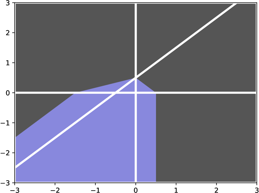
(a) The network’s linear partitions and decision boundaries before patching.

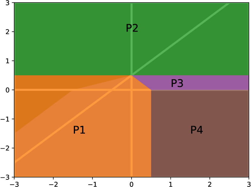
(b) The partitions used in the patch specification.

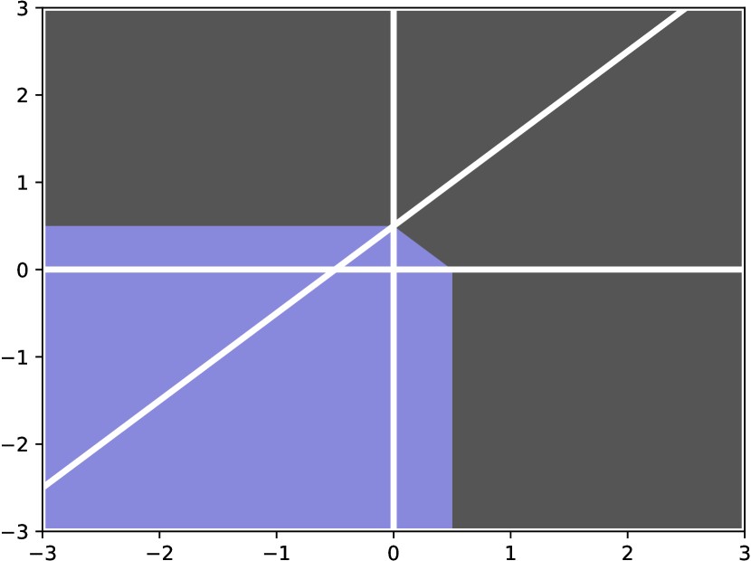
(c) The patched network’s linear partitions and decision boundaries.

Figure 5. Networking patching on DNN $f$ in Equation 3

7.1. Deep Neural Network Patching as a Non-Linear MAX SMT

The problem of finding such a patch can be seen as an instance of the more general MAX SMT problem, which looks to find values satisfying as many given logical formulas as possible. We recall from Definition 2 that we wish to find a $\delta$ satisfying: $\forall(X_{i},Y_{i})\in T:\forall x\in X_{i}:f(x;\theta+\delta)\in Y_{i}$, which can be directly translated to the MAX-SMT instance defined by the conjunction $\bigwedge_{(X_{i},Y_{i})\in T}\forall x\in X_{i}:f(x;\theta+\delta)\in Y_{i}$ (note that $x\in X_{i}$ and $y\in Y_{i}$ can be encoded in any theory supporting rational linear inequalities).

Although in theory this problem can be exactly solved by any modern SMT solver (such as Z3 (de Moura and Bjørner, 2008)), the extreme non-linearity involved makes it infeasible in practice. To make it feasible, we would like the problem to be highly linear, eg. encodable as an LP. Unfortunately, there are numerous reasons why this is not possible with the above formulation:

1. The constraints require that the theory solver can encode the network $f$, which is usually highly-non-linear (eg. ReLU layers introduce exponentially many possible branches).

2. It solves for $\delta$ while simultaneously quantifying over the infinite $x\in X_{i}$, resulting in significant non-linearity in the problem itself.

3. If $\delta$ can change multiple weights over multiple layers or nodes, the interaction between all weight changes results in a high-order polynomial problem instead of a linear one (because the linear layers are applied sequentially, eg. $y=w_{2}(w_{1}x+b_{1})+b_{2}$).

To address the first two of these problems, we will introduce in Section 7.2 a new neural network architecture termed Masking Networks. Our core result, Theorem 3, will show that Masking Networks have desirable properties which allow us to (1) replace the highly-non-linear $f$ with an affine map in each conjunct and (2) lower the problem of patching on the infinitely-many $x\in X_{i}$ with patching on finitely-many key points. To address the final issue, in Section 7.4 we will limit the set of weights that can be patched at the same time to ensure that the resulting problem is still linear. Finally, in Section 7.5 we will show that extending this restriction to only changing a single weight at a time (referred to as “weight-wise patching”) results in an algorithm efficient enough for use on real-world networks.

7.2. Masking Networks

Our central result in Theorem 3 relies on a new type of neural network, which we propose here and term a Masking Network. Masking Networks strictly generalizes the concept of a feed-forward network with ReLU activations and are loosely inspired by the work of Fiat et al. (2019). We note that the ideas in this section can be further extended to networks with arbitrary piecewise linear activation functions (eg. MaxPool) but we focus here on ReLU for ease of exposition. The essential insight is to fully separate the activation pattern of the network (which defines the partitioning of $\widehat{f}$) from the result of network (which defines the affine maps of $\widehat{f}$).

We first review the architecture of standard feed-forward neural networks, described in Section 2. The entire network function $f$ is decomposed into a series of sequentially-applied layers, which we denote $L_{1},L_{2},\ldots,L_{n}$. Given a particular input vector to the network, each layer is said to have an associated output vector. Namely, if $x$ is the input vector, then the output vector of layer $i$ is $L_{i}(\cdots L_{1}(x))$. Recall from Section 2.1 that, in a standard feed-forward ReLU network, the layers alternate between FullyConnected or 2DConvolution layers (which correspond to affine maps) and piecewise-linear ReLU layers, which are defined component-wise by:

$$\textsc{ReLU}{}(x)_{i}=\begin{cases}0&x_{i}\leq 0\\ x_{i}&x_{i}>0\end{cases}$$

Meaning that the $i$th component of the output vector is $0$ when the $i$th component of the input vector is non-positive, and left unchanged otherwise. An equivalent logical definition would be $(x_{i}>0\wedge\textsc{ReLU}{}(x)_{i}=x_{i})\vee(x_{i}\leq 0\wedge\textsc{ReLU}{}(x)_{i}=0)$.

In a Masking Network, four changes are made:

1. The inputs and outputs to each layer are vectors of 2-tuples $((x^{a}_{1},x^{v}_{2}),\ldots,(x^{a}_{d},x^{v}_{d}))$. In some scenarios it will be convenient to refer to the vector consisting of just the first-values, noted $x^{a}=(x^{a}_{1},\ldots,x^{a}_{d})$ and called the “activation vector.” Correspondingly, we will notate $x^{v}=(x^{v}_{1},\ldots,x^{v}_{d})$ and name this the “values vector.”

2. The input vector $x=(x_{1},\ldots,x_{k})$ to the entire network is converted to an input vector where the activation and values vectors are equal, i.e. $((x_{1},x_{1}),(x_{2},x_{2}),\ldots,(x_{k},x_{k}))$ or, equivalently, $x^{a}=x^{v}=x$.

3. The output of the network is taken to be only the values vector $x^{v}$ outputted by the last layer.

4. ReLU layers are replaced by Masked ReLU (MReLU) layers, defined below.

In a masking network, FullyConnected or 2DConvolution layers are associated with two parameters each, $\theta^{a}$ and $\theta^{v}$. Given an input with activation vectors $x^{a}$ and value vectors $x^{v}$ to a FullyConnected or 2DConvolution layer, $\theta^{a}$ and $\theta^{v}$ are applied to the $x^{a}$ and $x^{v}$ vectors independently as follows:

$$\textsc{FullyConnected}{}^{a}(x^{a},x^{v};\theta^{a},\theta^{v}) \buildrel\mbox{\tiny{def}}\over{=}\textsc{FullyConnected}(x^{a};\theta^{a})$$

$$\textsc{FullyConnected}{}^{v}(x^{a},x^{v};\theta^{a},\theta^{v}) \buildrel\mbox{\tiny{def}}\over{=}\textsc{FullyConnected}(x^{v};\theta^{v})$$

Given an input vector-of-tuples $((x^{a}_{1},x^{v}_{1}),\ldots,(x^{a}_{d},x^{v}_{d}))$ to a MReLU layer, we define its $i$th output tuple to be:

$$\textsc{MReLU}{}\left(\left((x^{a}_{1},x^{v}_{1}),\ldots,(x^{a}_{d},x^{v}_{d})\right)\right)_{i}=\begin{cases}(0,0)&x^{a}_{i}\leq 0\\ (x^{a}_{i},x^{v}_{i})&x^{a}_{i}>0\end{cases}$$

The following properties follow directly from these definitions and are integral to understanding Masking ReLU networks:

1. A masking network is piecewise-linear, and thus $\widehat{{f}_{\restriction X}}$ can be computed for any bounded polytope $X$ by Theorem 5.

2. If $x^{a}=x^{v}$, then $\textsc{MReLU}{}(x^{a},x^{v})=(\textsc{ReLU}{}(x^{v}),\textsc{ReLU}{}(x^{v}))$.

3. If $x^{a}=x^{v}$ and $\theta^{a}=\theta^{v}$, then $\textsc{FullyConnected}_{\theta^{a},\theta^{v}}(x^{a},x^{v})=$ $(\textsc{FullyConnected}_{\theta^{v}}(x^{v}),$ $\textsc{FullyConnected}_{\theta^{v}}(x^{v}))$ and similarly for 2DConvolution.

4. The value of the activation vectors ($x^{a}$) only ever depends on the values of prior activation vectors and activation parameters ($\theta^{a}$), never prior value vectors ($x^{v}$) or value parameters ($\theta^{v}$).

5. The non-linear behavior of the values vectors ($x^{v}$) is entirely controlled by the activation vectors ($x^{a}$). For example, if all activation vectors $x^{a}$ are strictly positive, then the entire masking network is affine (regardless of the values of the value vectors).

The first property allows us to use the symbolic representation $\widehat{f}$ of the masking network. The next two properties show that we can always encode any feed-forward ReLU network as a Masking ReLU network by setting $\theta^{a}=\theta^{v}=\theta$ for corresponding affine layers (i.e., masking networks are strictly more expressive than feed-forward ReLU networks). The final two properties ensure that:

1. The partitioning of $\widehat{f}$ is determined entirely by the activation parameters $\theta^{a}$.

2. The affine maps of $\widehat{f}$ are determined entirely by the value parameters $\theta^{v}$.

Intuitively, now, we can think of changes to the activation parameters $\theta^{a}$ as moving the positions of the partitions in $\widehat{f}$ (i.e., changing the position of the polytopes in Figure 2(a) and changing the position of the white lines in Figure 2(b) and Figure 5(a)). Moreover, changes to the value parameters $\theta^{v}$ corresponds to changing the classification within each partition (i.e., changing the position of the decision boundary within each white-line delineated region in Figure 2(b) and Figure 5(a) without changing the position of the white lines themselves).

7.3. Patching Deep Neural Networks on Infinite Inputs

The previous observations lead to the following theorem:

Theorem 3.

Given a masking network $f(x;\theta^{a},\theta^{v})$ parameterized by activation parameters $\theta^{a}$ and value parameters $\theta^{v}$, an input polytope $X$, output polytope $Y$, and $\widehat{{f}_{\restriction X}}=\{(P_{1},F_{1}),\ldots,(P_{n},F_{n})\}$, then:

A values-patched network $f(x;\theta^{a},\theta^{v}+\delta)$, modifying only $\theta^{v}$, satisfies the property $\forall x\in X:f(x;\theta^{a},\theta^{v}+\delta)\in Y$ if and only if it satisfies the property $\forall(P_{i},F_{i})\in\widehat{{f(x;\theta^{a},\theta^{v})}_{\restriction X}}:\forall v\in\mathrm{Vert}(P_{i}):F_{i}(v;\theta^{v}+\delta)\in Y$.

The above theorem, proved in Appendix I, allows us to translate the problem of patching over an infinite set of points to that of patching on finitely-many vertex points, as long as we keep the activation parameters $\theta^{a}$ constant. We will use this fact in Section 7.4 to phrase the patching problem as an instance of the linear MAX-SMT problem.

Finally, it is important to note that for any linear partition $(P_{i},F_{i})$ in the unpatched $\widehat{{f(x;\theta^{a},\theta^{v})}_{\restriction X}}$ we can compute $F_{i}(x;\theta^{v}+\delta)$ for any $\delta$, i.e. the affine map corresponding to the values-patched network $f(x;\theta^{a},\theta^{v}+\delta)$ over input region $P_{i}$. The existence of such a map follows from the observation that the linear partitioning of $\widehat{{f(x;\theta^{a},\theta^{v})}_{\restriction X}}$ is identical to that of $\widehat{{f(x;\theta^{a},\theta^{v}+\delta)}_{\restriction X}}$ because only the value parameters are modified (so linear partitions of the unpatched network are still linear partitions of the patched network.) The exact method of computing $F_{i}(x;\theta^{v}+\delta)$ is unimportant to this discussion, however for expository purposes we provide an example for the map corresponding to partition $P_{4}$ in Figure 5(b):

$$F(x\in P_{4};\theta+\delta)=\left(\begin{bmatrix}1&1&1\\ 0&-1&-1\end{bmatrix}+\delta^{3}\right)\begin{bmatrix}0&0&0\\ 0&1&0\\ 0&0&1\end{bmatrix}\left(\left(\begin{bmatrix}-1&1\\ 1&0\\ 0&1\end{bmatrix}+\delta^{1}\right)\begin{bmatrix}x_{1}\\ x_{2}\end{bmatrix}+\left(\begin{bmatrix}-0.5\\ 0\\ 0\end{bmatrix}+\delta^{2}\right)\right)+\left(\begin{bmatrix}0\\ 1\end{bmatrix}+\delta^{4}\right)$$

7.4. Network Patching as a Linear MAX SMT

In this section, we will show how Masking Networks can be used to address the issues identified in Section 7.1 and finally translate the highly-non-linear MAX SMT formulation of the patching problem into a linear one. To do this, we will restrict ourselves to only patching the $\theta^{v}$ value-parameters, and furthermore only patch the parameters for a single node at a time.

First, we translate the given ReLU network into an equivalent Masking Network (which can always be done as Masking Networks are strictly more powerful than sequential feed-forward networks). We can then address the problem (1) from Section 7.1, i.e. the non-linearity of $f$, by restricting ourselves to only patching the value parameters $\theta^{v}$. The value parameters do not impact the partitioning of $\widehat{f}$ (only the affine maps). Thus, this restriction allows us to break the non-linear MAX SMT query into a series of MAX SMT queries, one for each linear region, and within each the function is linear with respect to the input (see the discussion about $F_{i}(x;\theta^{v}+\delta)$ in Section 7.3).

To address problem (2) from Section 7.1, i.e. quantifying over the infinitely many $x\in X_{i}$ while solving for $\delta$, we use the result in Theorem 3 to quantify over the finitely-many vertices of each $X_{i}$ intersected with the linear region instead of over the infinitely-many points in each $X_{i}$. Theorem 3 ensures that the two are equivalent.

To address the final issue from Section 7.1, i.e. the non-linear interaction when changing multiple weights in a network, we can limit $\delta$ to only modify the weights corresponding to a single node in the network, which will prevent such non-linearity arising from sequential layers. Once all three of these changes are made, the corresponding satisfiability problem can be encoded as an LP and more general solvers like Z3 can find solutions to the maximization problem in some cases.

The corresponding satisfiability problem looks like:

(4) $$\bigwedge_{(X_{i},Y_{i})\in T}\bigwedge_{(P_{j},F_{j})\in\widehat{{f_{M}}_{\restriction X_{i}}}}\bigwedge_{v\in\textnormal{{Vert}}(P_{j})}F_{j}(v;\theta+\delta)\in Y_{i}$$

Where $f_{M}(\cdot;\theta,\theta)$ is the Masking Network equivalent to $f$, $F_{j}(v;\theta+\delta)$ is the affine map corresponding to $f_{M}(\cdot;\theta,\theta+\delta)$ over linear partition $P_{j}$, and $\delta$ changes the weights of at most a single node.

Notably, this involves finitely many conjunctions and $F_{j}(v;\theta+\delta)$ can be written as an affine function of $\delta$ when $v$ and $\theta$ are fixed. For example, consider again the expository network visualized in Figure 5 and the key point $(3,0.5)$ lying in polytope $P_{4}$. Now, if we only patch the second of the three nodes in the first affine layer, then $\delta$ has only three non-zero value (one for each of the $3$ inputs to that node along with its bias) which we can write $\delta_{1},\delta_{2},\delta_{3}$. We can then write $F_{1}(v;\theta,\theta+\delta)$ as:

$$F(x\in P_{4};\theta+\delta) =\begin{bmatrix}1&1&1\\ 0&-1&-1\end{bmatrix}\begin{bmatrix}0&0&0\\ 0&1&0\\ 0&0&1\end{bmatrix}\left(\begin{bmatrix}-1&1\\ 1+\delta_{1}&\delta_{2}\\ 0&1\end{bmatrix}\begin{bmatrix}3\\ 0.5\end{bmatrix}+\begin{bmatrix}-0.5\\ \delta_{3}\\ 0\end{bmatrix}\right)+\begin{bmatrix}0\\ 1\end{bmatrix}$$

$$=\begin{bmatrix}3\delta_{1}+0.5\delta_{2}+\delta_{3}\\ -3\delta_{1}-0.5\delta_{2}-\delta_{3}\end{bmatrix}+\begin{bmatrix}3.5\\ -2.5\end{bmatrix}$$

$$=\begin{bmatrix}3&0.5&1\\ -3&-0.5&-1\end{bmatrix}\begin{bmatrix}\delta_{1}\\ \delta_{2}\\ \delta_{3}\end{bmatrix}+\begin{bmatrix}3.5\\ -2.5\end{bmatrix}$$

which is clearly affine in the $\delta_{1},\delta_{2},\delta_{3}$ potentially-non-zero components of $\delta$. The exact derivation of the above matrices is not entirely important; instead, we wish to highlight that this formulation can translate the corresponding satisfiability problem into a linear one.

7.5. Weight-Wise Network Patching as an Interval MAX SMT

This linear formulation is still prohibitively expensive in most real-world scenarios, due primarily to the large number of “key points” necessary (often well over $30,000$). The last optimization we make to the process is to limit $\delta$ to changing only a single weight, which we refer to as “weight-wise patching.” Now, for any given weight in $\theta$, Equation 4 corresponds to a conjunction of linear inequalities in one variable. Thus, each of the conjuncts corresponds to an interval on the corresponding patch $\delta$ in which that constraint is met. We refer to the set of all such intervals for the $k$th weight as $I_{k}$. Finding the optimal patch for that weight now corresponds to finding an interval $M=[M^{l},M^{u}]$ that maximizes the number of intervals in $I_{k}$ that contain it. This can be done in linear time using a “linear sweep” algorithm once the intervals are sorted. We can repeat this process for every weight in a particular layer (or the entire network if desired), picking the weight and update which will satisfy the maximum number of constraints. Finally, we can greedily apply this algorithm to update multiple weights, at each step making the optimal change to a single weight in the network. Thus, this greedy algorithm is guaranteed to both monotonically increase the number of constraints met as well as terminate in a finite number of steps.

7.6. Efficiency of Patched Masking Networks

We close this section with a discussion of the inference-time efficiency of Masking Networks, in the process identifying another major benefit to weight-wise patching. On first glance, masking networks appear to double the amount of computation necessary to perform inference, and indeed, when there is no relation between the activation and value parameters ($\theta^{a}$ and $\theta^{v}$) this is the case. However, this is not necessarily the case when the parameterizations share many weight values. As an extreme example, we have already noted that when $\theta^{a}=\theta^{v}$, the network exactly corresponds to a normal ReLU network. As a slightly more complex example, if only a single weight in the last affine layer before a ReLU layer is changed, then the value of the corresponding node’s output activation and value vector coefficients differ by a constant difference in the weights multiplied by the corresponding input coefficient, incurring a cost of only one multiply-accumulate operation. In that way, if only a small number of weights differ between the values and activation network, the output of the masking network can be computed by keeping only “diffs” of the values of the nodes during inference. In Section 8.3, on two of our patch specifications we patched the last affine layer before the last ReLU layer (so at most one multiply-accumulate operation of overhead) and in another one we patched the very last affine layer, which is not followed by a ReLU layer, so there was no overhead at all.

8. Experimental Evaluations

In this section, we apply the techniques discussed in this paper to a number of interesting problems, comparing to prior work where applicable.

Tests were carried out on a dedicated Amazon EC2 c5.metal instance, using Benchexec (Beyer, 2016) to limit the number of CPU cores to 16 and RAM to 16GB. Our code is available at
https://github.com/95616ARG/SyReNN.

8.1. Understanding Network Behavior using Weakest Precondition

(a) Weakest precondition for Strong Right using $\widehat{{f}_{\restriction X}}$

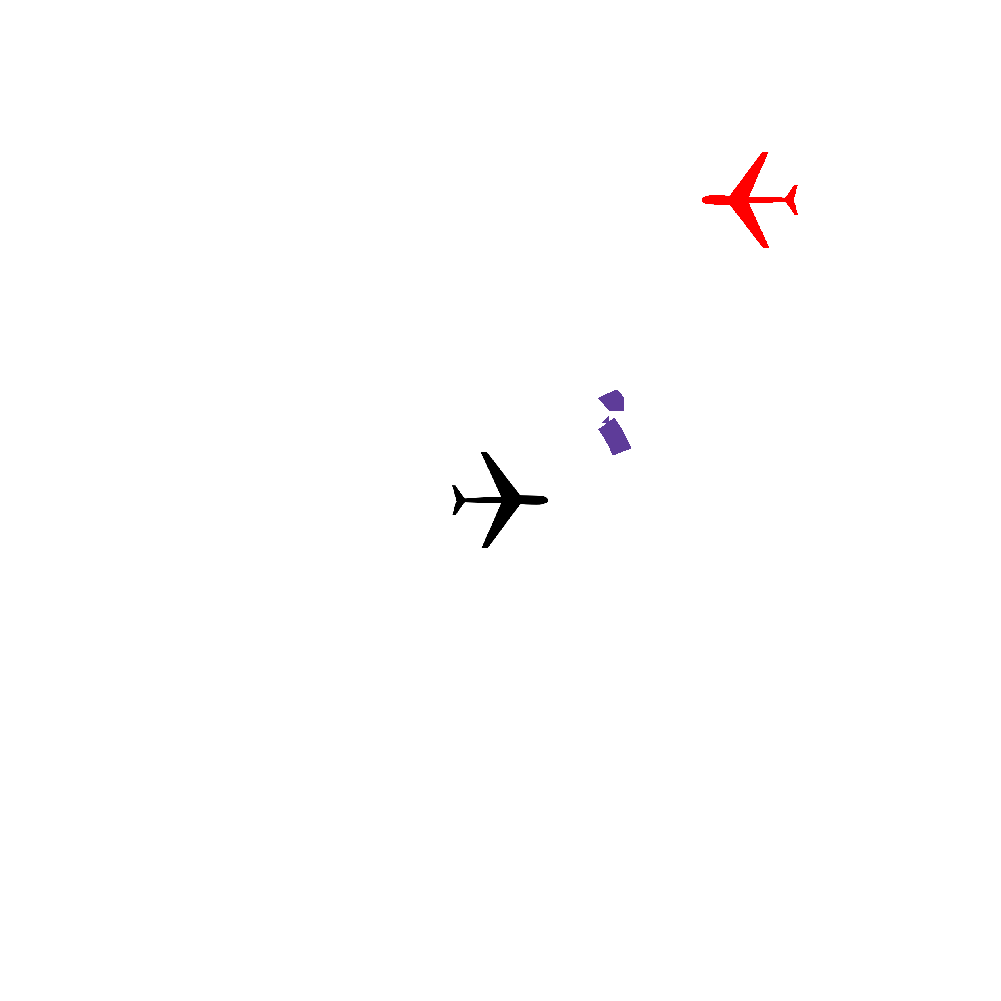
(b) Precondition for Strong Right using $\operatorname*{DPPre}[k=25]$

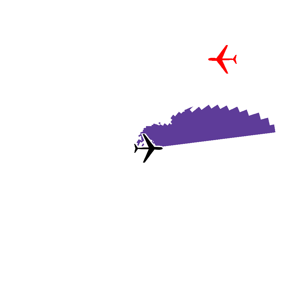
(c) Precondition for Strong Right using $\operatorname*{DPPre}[k=100]$

(d) Decision boundaries computed using $\widehat{{f}_{\restriction X}}$

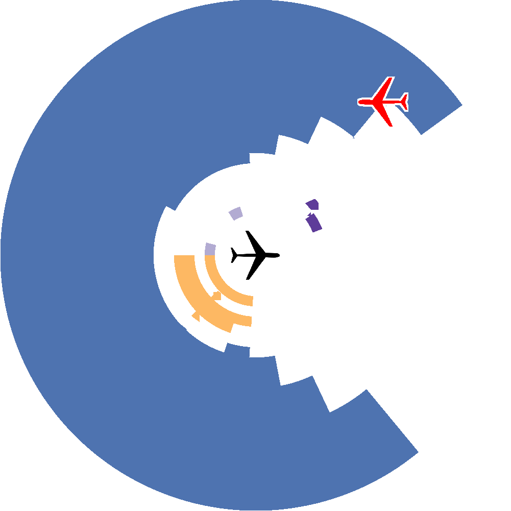
(e) Decision boundaries computed using $\operatorname*{DPPre}[k=25]$

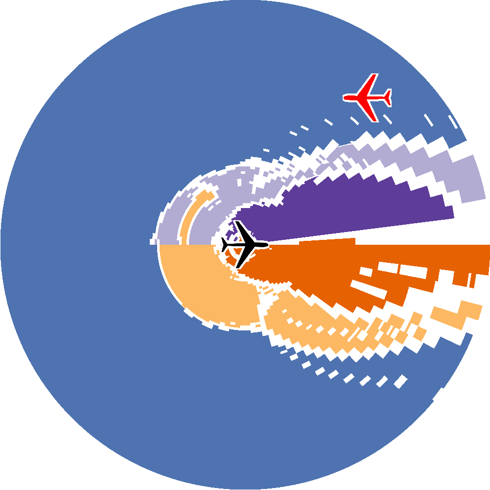
(f) Decision boundaries computed using $\operatorname*{DPPre}[k=100]$

Figure 6. Visualization of decision boundaries for the ACAS Xu network.

Legend:   Clear-of-Conflict,   Weak Right,   Strong Right,   Strong Left,   Weak Left.

Table 1. Performance of $\widehat{{f}_{\restriction X}}$ and $\operatorname*{DPPre}$ when used to compute weakest precondition and precondition for the ACAS Xu network (Julian et al., 2018). $\widehat{{f}_{\restriction X}}$ size is the number of partitions in the symbolic representation. $k$ is the number of splits used for $\operatorname*{DPPre}$; the number of partitions used is then $k^{2}$. Each scenario represents a different two-dimensional slice of the input space; within each slice, the heading of the intruder relative to the ownship along with the speed of each involved plane is fixed.

			$\operatorname*{DPPre}$ time (secs)
Scenario	$\widehat{{f}_{\restriction X}}$ size	$\widehat{{f}_{\restriction X}}$ time (secs)	k = 25	k = 55	k = 100
Head-On, Slow	33200	10.9	9.1	43.2	141.3
Head-On, Fast	30769	10.2	8.2	39.0	128.0
Perpendicular, Slow	37251	12.5	9.2	42.9	141.7
Perpendicular, Fast	33931	11.4	8.2	39.2	127.5
Opposite, Slow	36743	12.1	9.8	46.7	152.5
Opposite, Fast	38965	13.0	9.5	45.2	147.3
-Perpendicular, Slow	36037	11.9	9.5	45.0	146.4
-Perpendicular, Fast	33208	10.9	8.3	39.5	130.2

For this application, we wanted to investigate the following two research questions:

1. Can we efficiently visualize the decision boundaries of an ACAS Xu aircraft-avoidance network using $\widehat{{f}_{\restriction X}}$?

2. How does prior work ($\operatorname*{DPPre}[k]$ using DeepPoly (Singh et al., 2019)) compare, both in efficiency and precision, when used to compute $\textsc{Pre}({f}_{\restriction X},Y)$?

To investigate these concerns, we wrote programs to compute $\textsc{WPre}({f}_{\restriction X},Y)$ and $\textsc{Pre}({f}_{\restriction X},Y)$ for arbitrary polytopes $X$ and $Y$ using $\widehat{{f}_{\restriction X}}$ (Section 5.3) and $\operatorname*{DPPre}$ (Section 5.2), respectively. Then, for each of the possible advisories produced by the network, we plotted the precondition set in a human-visualizable form, with the results shown in Figure 6(f). Notably, the precision when using $\operatorname*{DPPre}[k]$ increases when the input domain is pre-partitioned (i.e., $k>1$), with the analysis being performed on each partition independently. Thus, we have shown a progression of plots from the $\operatorname*{DPPre}[k]$ approach, each one using progressively more partitions $k$ for $\operatorname*{DPPre}[k]$ (all converging to the weakest precondition found using $\widehat{{f}_{\restriction X}}$). Note that, as we used a two-dimensional input region, $\operatorname*{DPPre}[k]$ uses $k^{2}$ separate partitions and calls to $\operatorname*{DPPre}[1]$.

The imprecision from using DeepPoly in $\operatorname*{DPPre}$ (see Figure 6(f)) is to be expected, as its symbolic representation was designed to efficiently answer decision (yes/no) queries about relatively small regions of a high-dimensional input space. By contrast, in this experiment we are stretching the DeepPoly representation beyond that goal by extracting preconditions over large regions of a low-dimensional input space.

Table 1 shows the time taken by each analysis. Note that the time taken does not include plotting time; only the time necessary to compute the precondition sets. As we increase the number of partitions (equal to $k^{2}$) used by $\operatorname*{DPPre}$, the precision goes up (as shown in Figures 6(b)-6(c)) but so does the time taken for analysis. We find that, except for very small $k$ where the precondition set is nearly-empty, the $\operatorname*{DPPre}$ analysis is slower than that using $\widehat{{f}_{\restriction X}}$ (which provides the exact $\textsc{WPre}({f}_{\restriction X},Y)$).

Both of these results match our expectations; $\widehat{{f}_{\restriction X}}$ is well-suited for immediately determining $\textsc{WPre}({f}_{\restriction X},Y)$, while attempting to use the DeepPoly representation (which is optimized for the decision procedure case) is advisable only when precision is not particularly important.

8.2. Bounded Model Checking of Safety Properties using Strongest Postcondition

For this application, we wanted to investigate the following two research questions:

1. Can we use $\widehat{{f}_{\restriction X}}$ to efficiently perform bounded model checking on a neural-network controller?

2. How efficient is prior work (ReluPlex (Katz et al., 2017)) at performing bounded model checking on a neural-network controller?

(a) Pendulum

(b) Quadcopter

(c) Satelite

Figure 7. Performance of bounded model checking (BMC) for three neural-network controllers using $\widehat{{f}_{\restriction X}}$ (blue line) and ReluPlex (red line). The x-axis is the number of steps used in BMC, y-axis is the time taken in seconds. A timeout of 1 hour was used. For the Pendulum model, the $\widehat{{f}_{\restriction X}}$ approach stopped after finding a counter-example on the 51st step (after approximately 30 minutes).

Table 2. Maximum number of steps verified by $\widehat{{f}_{\restriction X}}$ and ReluPlex approaches for BMC before timeout. Timeout was set to 1 hour. “*” indicates a counter example was found after that many steps.

Model	$\widehat{{f}_{\restriction X}}$ Steps	ReluPlex Steps
Pendulum	51*	2
Quadcopter	25	6
Satelite	13	4

To answer these questions, we chose a subset of neural-network controller models from (Zhu et al., 2019) that have two-dimensional states and affine state-transition functions. We utilized the initial, safe, and unsafe sets from that work. As an initial optimization, we removed from the initial set any states which could be guaranteed (based only on the environment dynamics and maximum/minimum output bounds on the network controller) to map into the initial set after one timestep. This resulted in a disjunctive initial state.

We then performed bounded model checking of the models using ReluPlex (Katz et al., 2017) and $\widehat{{f}_{\restriction X}}$ as described in Section 6. Figure 7 shows the time taken to perform the analysis for each network up to a given timestep of the model, while Table 2 summarizes these results.

As we can see, bounded model checking with $\widehat{{f}_{\restriction X}}$ can be significantly more efficient than using ReluPlex. This is primarily because the approach using $\widehat{{f}_{\restriction X}}$ directly computes the strongest postcondition on network output after each step, which can then be re-used efficiently in the strongest-postcondition computation for the next timestep. By contrast, re-use between timestep computations for ReluPlex is not possible, meaning verifying each progressive timestep becomes progressively more challenging.

8.3. Patching Deep Neural Networks

(a) “Pockets” Specification

(b) “Bands” Specification

(c) “Symmetry” specification.

Figure 8. Weights changed vs. percent of constraints met. The blue line shows the percent of constraints met on the input slice that the patch targeted, while the red line shows the percent of constraints met on a slice at higher velocity.

Table 3. Summarizes the percent of constraints met and time taken per iteration for patching three specifications. “Patched Slice” is the input domain of interest that the patch spec applies to, while “Other Slice” shows how patching one slice can generalize to patches for another.

	Constraints Met
	Patched Slice		Other Slice		Time Per Iteration
Patch	Initial	Final	Initial	Final	Mean	Std. Dev.
Pockets	99.6%	99.994%	99.3%	99.7%	23.6	15.2
Bands	99.6%	99.98%	99.7%	99.8%	15.9	2.3
Symmetry	88.5%	97.0%	88.9%	95.6%	4.7	0.1

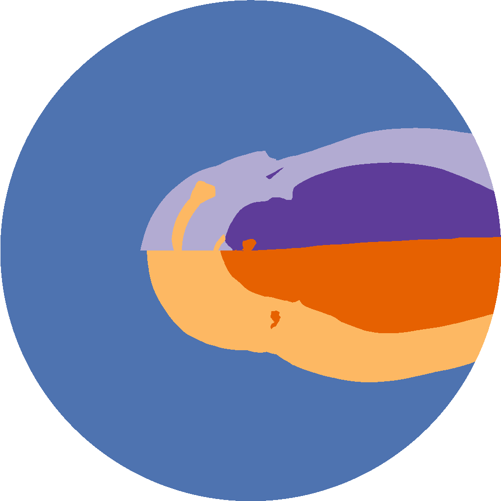
(a) Before patching.

(b) After one iteration (weight change).

(c) After five iterations (weight changes).

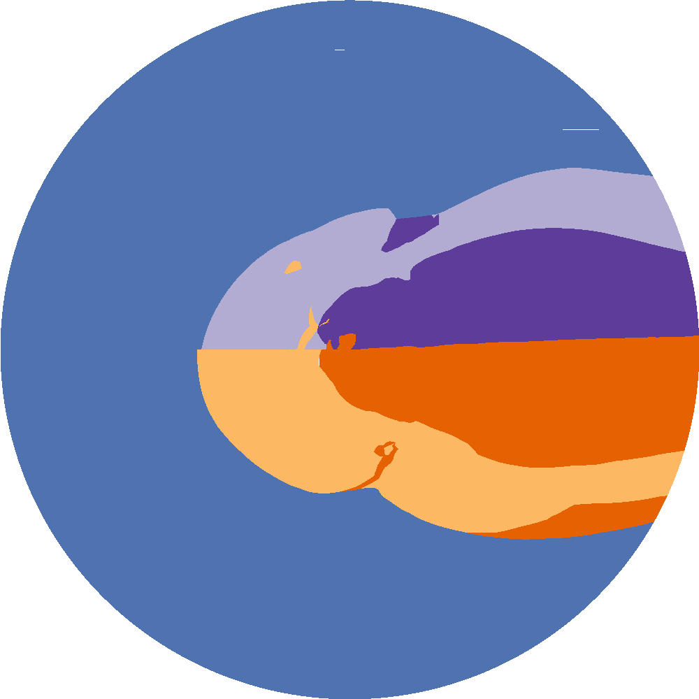
(d) Before patching (generalization region).

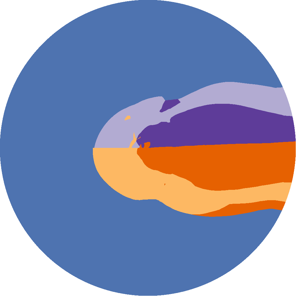
(e) Generalization after one iteration (weight change) on the patch region.

(f) Generalization after five iterations (weight change) on the patch region.

Figure 9. Network patching for the “Pockets” spec (Removing the “pockets” of strong-left and strong-right).

Legend:   Clear-of-Conflict,   Weak Right,   Strong Right,   Strong Left,   Weak Left.

(a) Before patching.

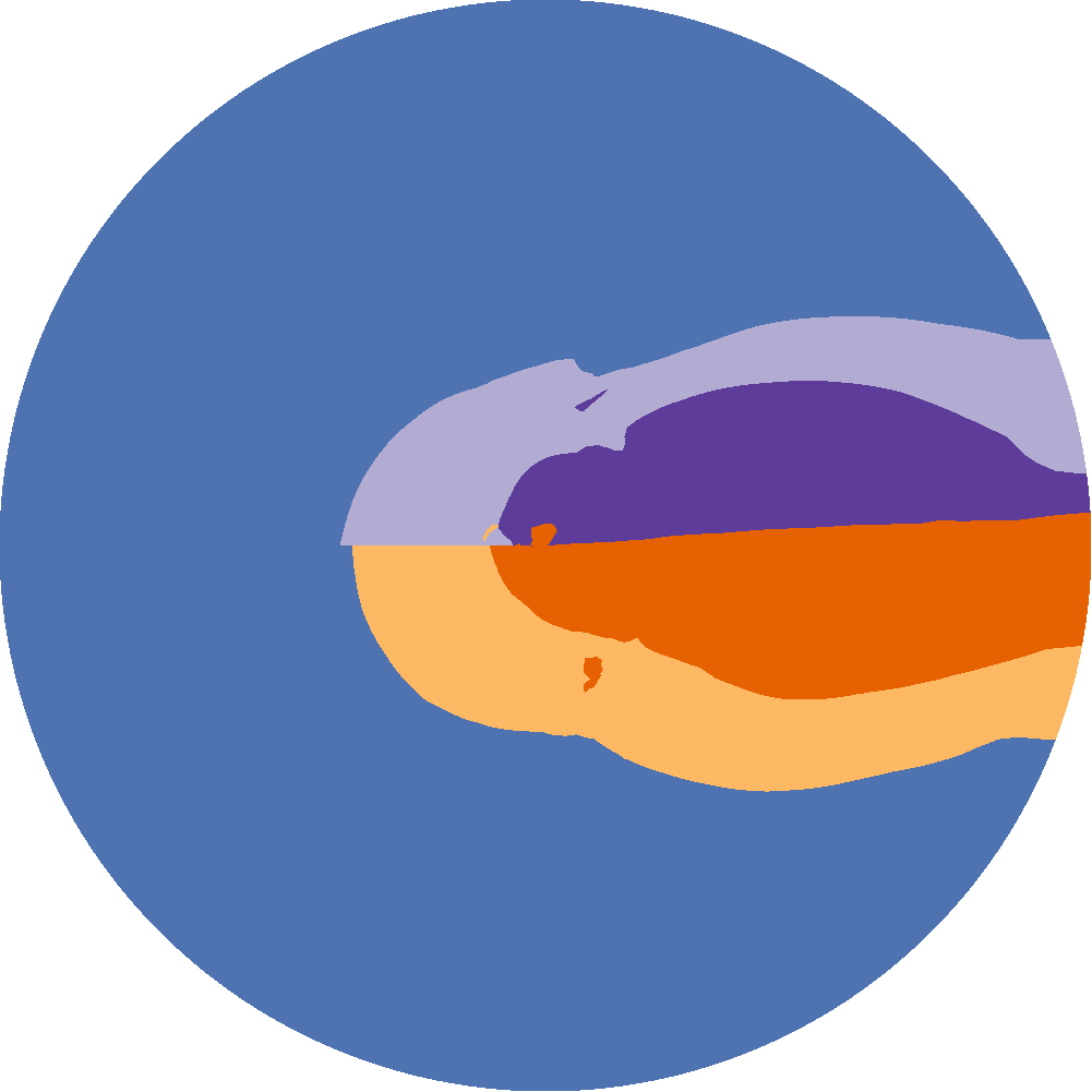
(b) After one iteration (weight change).

(c) After five iterations (weight changes).

(d) Before patching (generalization region).

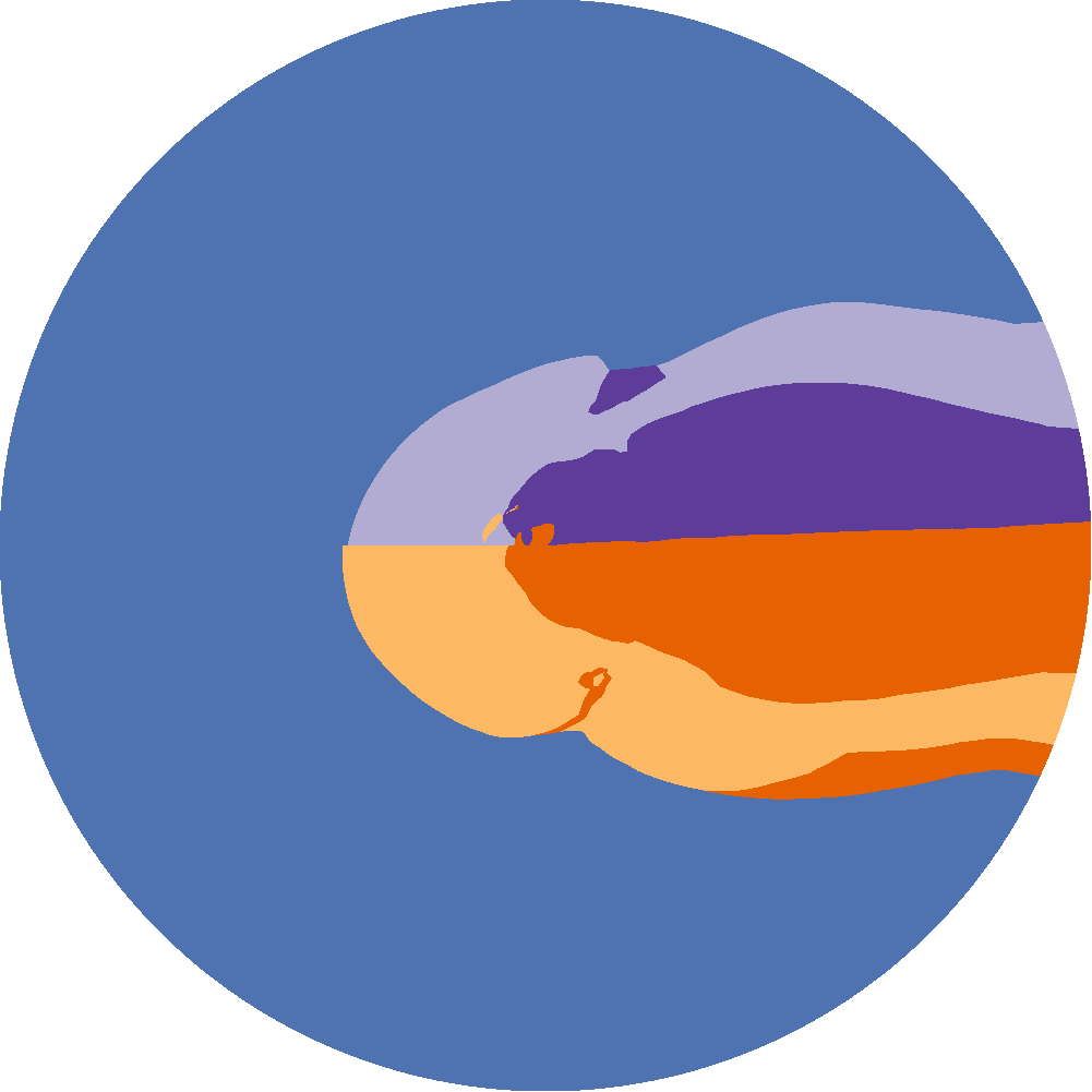
(e) Generalization after one iteration (weight change) on the patch region.

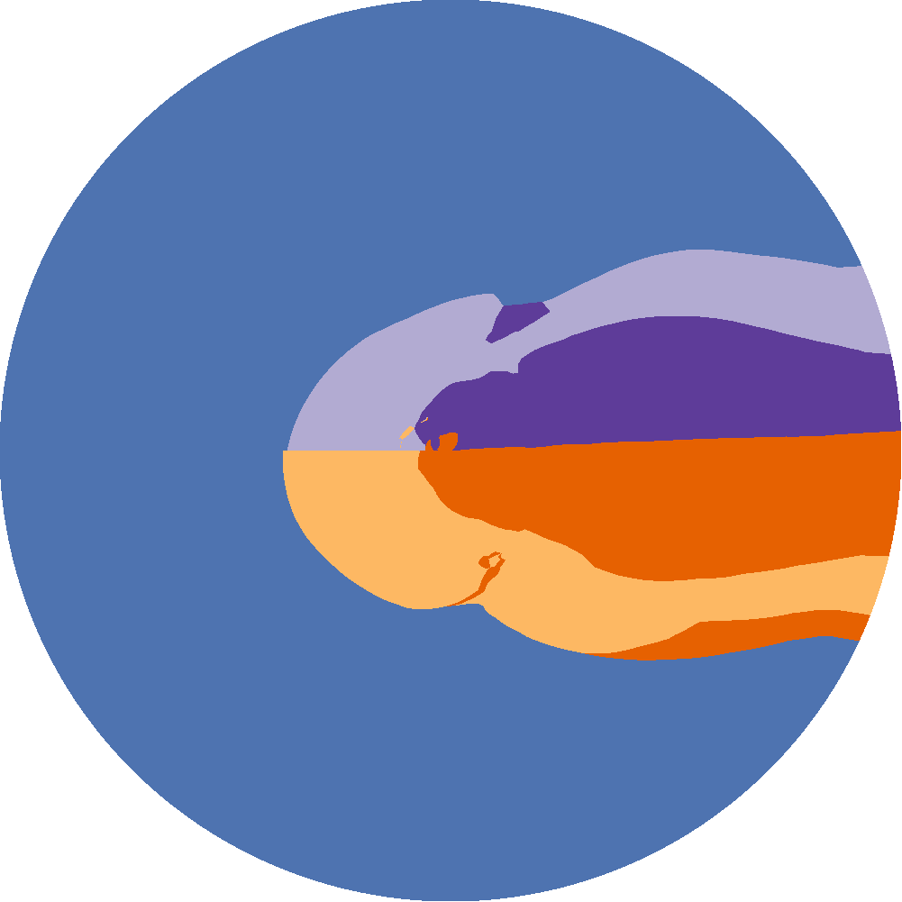
(f) Generalization after five iterations (weight change) on the patch region.

Figure 10. Network patching for the “Bands” spec (Removing the band of weak-left behind the origin).

Legend:   Clear-of-Conflict,   Weak Right,   Strong Right,   Strong Left,   Weak Left.

(a) Before patching.

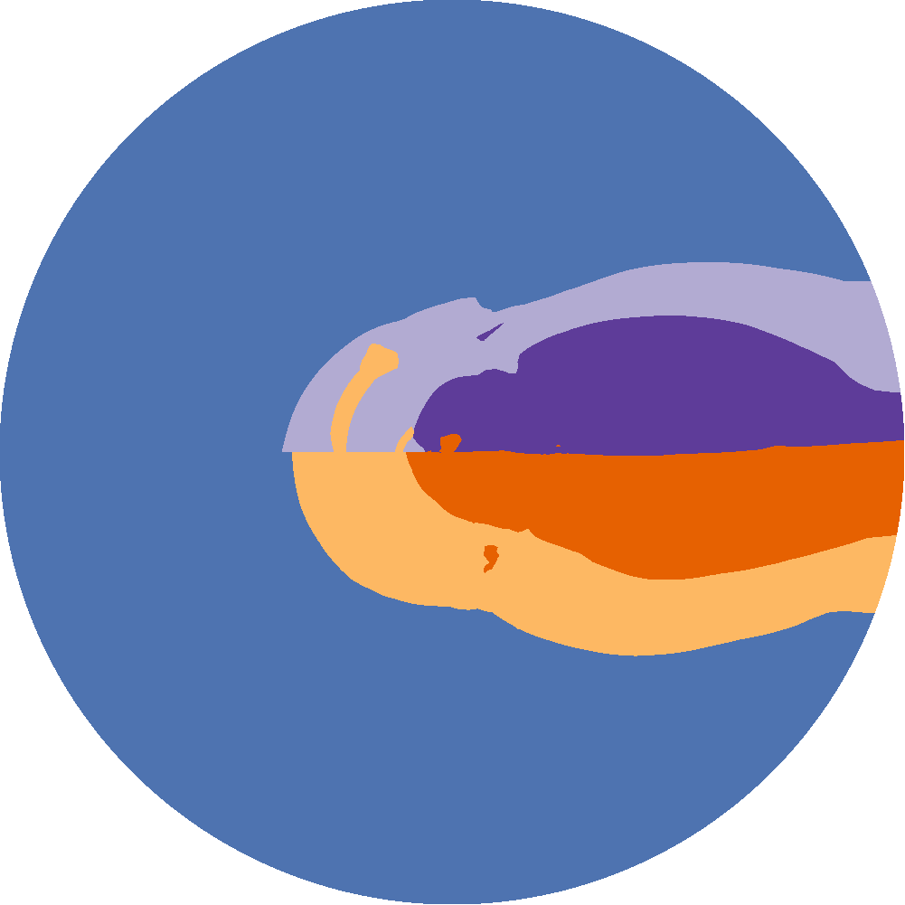
(b) After one iteration (weight change).

(c) After five iterations (weight changes).

(d) Before patching (generalization region).

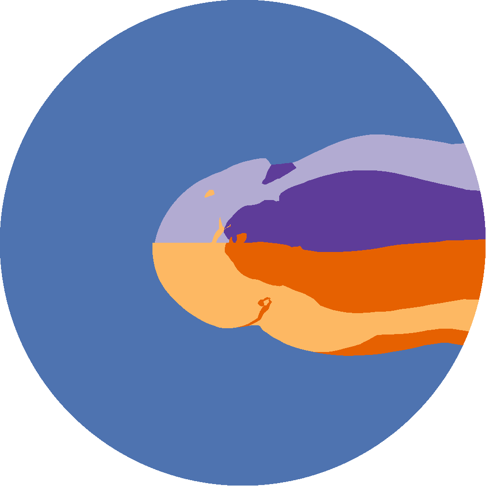
(e) Generalization after one iteration (weight change) on the patch region.

(f) Generalization after five iterations (weight change) on the patch region.

Figure 11. Network patching for the “Symmetry” spec (Lowering the main decision boundary between strong-left and strong-right to become symmetrical).

Legend:   Clear-of-Conflict,   Weak Right,   Strong Right,   Strong Left,   Weak Left.

For this application, we wanted to understand the following three research questions:

1. Can an ACAS Xu network be patched to correct a number of undesired behaviors?

2. How well do patches on a single two-dimensional subsets of the input space generalize to (i.e. fix the same behavior on) other subsets of the input space?

3. How well does the greedy MAX-SMT solver described in 7.1 work, both in terms of efficiency and optimization?

To answer the first two questions, we took the ACAS Xu network visualized in Figure 6(f) and attempted to patch three suspicious behaviors of the network using the approach described in Section 7. The “Pockets” patch specification (Figure 9(f)) attempts to get rid of the “pockets” of strong left/strong right in regions that are otherwise weak left/weak right. The “Bands” specification (Figure 10(f)) attempts to get rid of the weak-left region behind and to the left of the ownship (at the origin). The “Symmetry” specification (Figure 11(f)) attempts to lower the decision boundary between strong left/strong right to be symmetrical.

After patching, we plotted the patched network in the same two-dimensional region it was originally plotted (and then patched) over, as well as another two-dimensional region formed by increasing the velocities of the ownship and attacking ship by $50$ kilometers per hour (to evaluate generalization to input regions not explicitly patched). The before and after plots are presented in Figure 9(f), Figure 10(f), and Figure 11(f).

To answer the third question quantitatively, we timed the performance on the three evaluations shown above and present it in Table 3 along with the percent of constraints met at each step in Figure 8.

We find that our proposed approach works very well; by changing only five weights, we were able to near-perfectly apply most of the patches (eg. notice the disappearance of the “offending” regions between Figure 9(a) and Figure 9(c)). Furthermore, for the most part, the patches appear to generalize to regions not explicitly considered in the patching process (eg. notice the disappearance of the out-of-place “strong left” region between Figure 9(d) and Figure 9(e) after changing only a single weight). The efficacy of the greedy MAX-SMT solver is further exemplified by the quantitative results in Table 3 and Figure 8, which shows that it is very effective at quickly meeting a large fraction of the desired constraints. However, patching was not, in general, a “silver bullet,” and sometimes undesired changes were introduced (cf. Figure 11(f), which has introduced a small “strong right” region into what was otherwise “weak left” on the generalized region). Avoiding such issues is an interesting direction for future work, but for the most part, we believe the results shown here to be extremely promising for the application of network patching in practice.

9. Related Work

This section describes prior work relevant to each of the contributions of this paper (Section 1.2).

A symbolic representation of deep neural networks  Xiang et al. (2017) solve the problem of exactly computing the reach set of a neural network given an arbitrary convex input polytope. However, the authors use an algorithm that relies on explicitly enumerating all exponentially-many ($2^{n}$) possible signs at each ReLU layer. By contrast, our algorithm adapts to the actual input polytopes, efficiently restricting its consideration to activations that are actually possible.

Thrun (1994) presents an early approach for extraction of if-then-else rules from artificial neural networks. Bastani et al. (2018) learn decision tree policies guided by a DNN policy that was learned via reinforcement learning. This decision tree could be seen as a particular form of symbolic representation of the underlying DNN.

Understanding network behavior using weakest precondition.  Because DNNs are difficult to meaningfully interpret, researchers have tried to understand the behavior of such networks. For instance, networks have been shown to be vulnerable to adversarial examples—inputs perturbed in a way imperceptible to humans but which are misclassified by the network (Szegedy et al., 2014; Goodfellow et al., 2015; Moosavi-Dezfooli et al., 2016; Carlini and Wagner, 2018)–and fooling examples—inputs that are completely unrecognizable by humans but recognized by DNNs (Nguyen et al., 2015). Breutel et al. (2003) presents an iterative refinement algorithm that computes an overapproximation of the weakest precondition as a polytope where the required output is also a polytope.

Bounded model checking of safety properties using strongest postcondition.  Scheibler et al. (2015) verify the safety of a machine-learning controller with BMC using the SMT-solver iSAT3, but support small unrolling depths and basic safety properties. Zhu et al. (2019) use a synthesis procedure to generate a safe deterministic program that can enforce safety conditions by monitoring the deployed DNN and preventing potentially unsafe actions. The presence of adversarial and fooling inputs for DNNs as well as applications of DNNs in safety-critical systems has led to efforts to verify and certify DNNs (Bastani et al., 2016; Katz et al., 2017; Ehlers, 2017; Huang et al., 2017; Gehr et al., 2018; Bunel et al., 2018; Weng et al., 2018; Singh et al., 2019; Anderson et al., 2019). Approximate reachability analysis for neural networks safely overapproximates the set of possible outputs (Gehr et al., 2018; Xiang et al., 2017, 2018; Weng et al., 2018; Dutta et al., 2018; Wang et al., 2018).

Patching deep neural networks.  Prior work focuses on enforcing constraints on the network during training. DiffAI (Mirman et al., 2018) is an approach to train neural networks that are certifiably robust to adversarial perturbations. DL2 (Fischer et al., 2019) allows for training and querying neural networks with logical constraints.

10. Conclusion

We proposed a symbolic neural network representation, denoted $\widehat{f}$, which decomposes a piecewise-linear neural network into its constituent affine maps. We applied this symbolic representation to three problems relating to trained neural networks. First, we showed how the representation can be used to compute weakest preconditions, which allow one to exactly visualize network decision boundaries. Next, we demonstrated the symbolic representation’s use for computing strongest postconditions, allowing us to perform iterative bounded model checking. Finally, we introduced the problem of patching neural networks, which can be interpreted as explicitly correcting their decision boundaries. We presented an efficient and effective approach to patching neural networks, relying on a new neural network architecture, the symbolic representation, and a dedicated MAX SMT solver.

Appendix A Theorem 2

See 2

Proof.

One such function is $f(x)=x^{2}$, which is clearly differentiable everywhere with $\frac{d}{dx}f=2x$.

Suppose there existed some $\widehat{f}=\{(P_{1},F_{1}),(P_{2},F_{2}),\ldots,(P_{n},F_{n})\}$. Then, as the domain of $f$ is infinite ($\mathbb{R}$) and is partitioned with finitely many polytopes, at least one $P_{i}$ must have infinitely many (and thus more than one) distinct points.

Now, consider any two points $x_{1}\neq x_{2}\in P_{i}$. Then we have:

(5) $$\left(\frac{x_{1}+x_{2}}{2}\right)^{2}=F_{i}\frac{x_{1}+x_{2}}{2}$$

$$\implies \frac{x_{1}^{2}+2x_{1}x_{2}+x_{2}^{2}}{4}=\frac{F_{i}x_{1}+F_{i}x_{2}}{2}$$

$$\implies \frac{x_{1}^{2}+2x_{1}x_{2}+x_{2}^{2}}{4}=\frac{x_{1}^{2}+x_{2}^{2}}{2}$$

$$\implies x_{1}^{2}+2x_{1}x_{2}+x_{2}^{2}=2x_{1}^{2}+2x_{2}^{2}$$

$$\implies 2x_{1}x_{2}=x_{1}^{2}+x_{2}^{2}$$

$$\implies 0=x_{1}^{2}-2x_{1}x_{2}+x_{2}^{2}$$

$$\implies 0=(x_{1}-x_{2})^{2}$$

$$\implies x_{1}=x_{2}$$

Which contradicts our assumption that $x_{1}\neq x_{2}$. ∎

Appendix B Theorem 3

See 3

Proof.

We observe that the argument from Theorem 2 holds here as well; if $X$ is a non-singleton, non-empty polytope, then it contains infinitely many points and so any finite partitioning of it will have at least one partition containing more than one distinct point. From there, the proof is identical. ∎

Appendix C Theorem 4

See 4

Proof.

Consider the function $f(x_{1},x_{2})=x_{1}^{2}-x_{2}^{2}=(x_{1}+x_{2})(x_{1}-x_{2})$ and the bounded polytope $X$ defined by $\{x\mid 0\leq x_{1}\leq 1\wedge x_{1}-x_{2}=1\}$.

We first show that $\widehat{f}$ does not exist. Suppose $\widehat{f}=\{(P_{1},F_{1}),\ldots,(P_{n},F_{n})\}$ exists. Then, it holds that:

$$\widehat{{f}_{\restriction Z}}=\{(P_{1}\cap Z,F_{1}),\ldots,(P_{n}\cap Z,F_{n})\}$$

Also exists, where $Z$ is the convex polytope defined by $x_{2}=0$. However, ${f}_{\restriction Z}=f(x_{1},0)=x_{1}^{2}$, so this implies that $\widehat{(x\mapsto x^{2})}$ exists, contradicting the proof of non-existence given in Theorem 2.

Finally, we show that $\widehat{{f}_{\restriction X}}$ does exist, where $X=\{x\mid x_{1}\leq 1\wedge x_{1}-x_{2}=1$. In that case, all $x$ values satisfy $x_{1}-x_{2}=1$, so $f(x)=(x_{1}+x_{2})(x_{1}-x_{2})=x_{1}+x_{2}$, which is affine. Thus $\widehat{{f}_{\restriction X}}=\{(X,x\mapsto x_{1}+x_{2})\}$ is a valid solution. ∎

Appendix D Theorem 5

See 5

Proof.

Let our piecewise-linear function have linear regions $\{R_{1},\ldots,R_{k}\}$ with associated affine maps $\{M_{1},\ldots,M_{k}\}$.

Let $\widehat{g}=\{(P_{1},F_{1}),\ldots,(P_{m},F_{m})\}$.

We note that, because the $P_{i}$s partition the domain of $g$, it suffices to show the construction on any of the $(P_{i},F_{i})$ pairs individually; the union of the results for each $(P_{i},F_{i})$ pairs will form $f\otimes\widehat{g}$.

Now, consider any $(P_{i},F_{i})$ pair in $\widehat{g}$. We compute the post-set of $P_{i}$ under $F_{i}$:

$$Y_{i}=\{F_{i}x\mid x\in P_{i}\}$$

Which is a convex polytope, the vertices of which can be computed by applying $F_{i}$ to each of the finitely-many vertices of $P_{i}$ (this a well-known fact in convex geometry).

Next, we compute $Y^{j}_{i}=Y_{i}\cap R_{j}$, where $R_{j}$ again is the $j$th linear region of $f$ associated with map $B_{j}$. This again is computable, as there are finitely many such $R_{j}$s and the intersection of two convex polytopes can be computed by conjunction of their half-space faces.

We have now partitioned $Y_{i}$ according to the linear regions of $f$, all that remains is to find a corresponding partitioning of $P_{i}$ such that each partition $P^{j}_{i}$ maps to $Y^{j}_{i}$ under $F_{i}$.

For each vertex $v_{l}$ of $Y^{j}_{i}$, we then compute $c_{l}$, a convex combination of the vertices of $Y_{i}$ that forms $v_{l}$, i.e. $\mathrm{Vert}(Y_{i})\cdot c_{l}=v_{l}$. Notably, to deal with non-invertible $F_{i}$ maps, when multiple $Y^{j}_{i}$ share the same vertex $v_{l}$, we must pick the same combination $c_{l}$ (which can be accomplished via a memo dictionary of previously found $(v_{l},c_{l})$ pairs). Furthermore, when $v_{l}$ is also a vertex of $Y_{i}$, we must use the corresponding vertex from $P_{i}$.

Now, for each of the $(v_{l},c_{l})$ pairs, we compute $p_{l}=\mathrm{Vert}(P_{i})c_{l}$. We note that, because $F_{i}$ is affine:

$$F_{i}(p_{l})=F_{i}(\mathrm{Vert}(P_{i})c_{l})=\mathrm{Vert}(Y_{i})c_{l}=v_{l}$$

We note now that the $p_{l}$s partition $P_{i}$ because the $v_{l}$s partition $Y_{i}$ and we mapped each $v_{l}$ back uniquely to a $p_{l}$ (mapping vertices to vertices where applicable). We now define:

$$P^{j}_{i}=\{p_{l}\mid\text{ the corresponding }v_{l}\text{ is a vertex of }Y^{j}_{i}\}$$

Finally, we claim that:

$$\widehat{f\circ g}=\{(P^{1}_{i},M_{1}\circ A_{i}),(P^{2}_{i},M_{2}\circ A_{i}),\ldots,(P^{k}_{i},M_{k}\circ A_{i})\mid 1\leq i\leq m\}$$

This follows as all points in $P_{i}$ are first mapped to $F_{i}x\in Y^{j}_{i}$ by $g$ then each point $F_{i}x$ in $Y^{j}_{i}$ is mapped to $B_{j}(A_{i}x)=(B_{j}A_{i})x$ by the application of $f$. ∎

Appendix E Corollaries 6—10

These follow as all of the described functions are well-known to be piecewise-linear.

Appendix F Corollary 11

See 11

Proof.

Let the layers be $l_{1},l_{2},\ldots,l_{n}$ such that $f=l_{n}\circ l_{n-1}\circ\cdots\circ l_{1}$.

Now, we have:

$$l_{n}\otimes\cdots\otimes l_{2}\otimes l_{1}\otimes\widehat{g} =l_{n}\otimes\cdots\otimes l_{2}\otimes\widehat{(l_{1}\circ g)}$$

$$=l_{n}\otimes\cdots\otimes\widehat{(l_{2}\circ l_{1}\circ g)}$$

$$\vdots$$

$$=\widehat{(l_{n}\circ\cdots\circ l_{1}\circ g)}$$

$$=\widehat{(f\circ g)}$$

$$=f\otimes\widehat{g}$$

Thus, $f\otimes\widehat{g}$ is computable by repeated application of $l_{i}\otimes\cdot$ for descending $i>0$, and $l_{i}\otimes\cdot$ was shown computable in Corollaries 6—10. ∎

Appendix G Theorem 1

See 1

Proof.

It is well-known in computational geometry that the vertices of the intersection of a polytope with a hyperplane is the intersection of its edges with the plane. The algorithm computes the ratio along each edge that the intersection is reached using standard linear algebra, i.e.:

$$(Q+\alpha(R-Q))_{d}=0$$

$$\implies Q_{d}+\alpha(R_{d}-Q_{d})=0$$

$$\implies \alpha=-\frac{Q_{d}}{R_{d}-Q_{d}}$$

Because $F$ is affine, the ratio holds when taking the preimage as well (which is what is returned). ∎

Appendix H Theorem 2

See 2

Proof.

It suffices to show that the algorithm correctly partitions each input polytope $P$ such that the signs within a partition are constant. Notably, because of convexity, it suffices to show that the signs of the vertices of each partition are constant.

We maintain two invariants every time we process some $P,F$ pair from the queue. The first is that the corresponding polytope will only be added to $Y$ if the signs of all vertices are constant (or zero). The second is that at each step, we partition the polytope into two new ones (using SplitPlane) such that fewer sign switches happen in each than the original polytope. This follows from the correctness of the SplitPlane algorithm.

The first invariant ensures that, if it halts, the algorithm is correct. The second ensures that it will halt, as there are only finitely many dimensions to consider. ∎

Appendix I Theorem 3

See 3

Proof.

This follows as the function within each partition is affine, and thus convex. If all of the vertices fall inside of $Y$, then by definition of convexity all of the interior points must as well (and vice-versa). ∎