A Fast and Efficient Stochastic Opposition-Based Learning for Differential Evolution in Numerical Optimization

Abstract

A fast and efficient stochastic opposition-based learning (OBL) variant is proposed in this paper. OBL is a machine learning concept to accelerate the convergence of soft computing algorithms, which consists of simultaneously calculating an original solution and its opposite. Recently, a stochastic OBL variant called BetaCOBL was proposed, which is capable of controlling the degree of opposite solutions, preserving useful information held by original solutions, and preventing the waste of fitness evaluations. While it has shown outstanding performance compared to several state-of-the-art OBL variants, the high computational cost of BetaCOBL may hinder it from cost-sensitive optimization problems. Also, as it assumes that the decision variables of a given problem are independent, BetaCOBL may be ineffective for optimizing inseparable problems. In this paper, we propose an improved BetaCOBL that mitigates all the limitations. The proposed algorithm called iBetaCOBL reduces the computational cost from $O(NP^{2}\cdot D)$ to $O(NP\cdot D)$ ($NP$ and $D$ stand for population size and a dimension, respectively) using a linear time diversity measure. Also, the proposed algorithm preserves strongly dependent variables that are adjacent to each other using multiple exponential crossover. We used differential evolution (DE) variants to evaluate the performance of the proposed algorithm. The results of the performance evaluations on a set of 58 test functions show the excellent performance of iBetaCOBL compared to ten state-of-the-art OBL variants, including BetaCOBL.

1 Introduction

An evolutionary algorithm (EA) is a subset of evolutionary computation, which is a nature-inspired optimization technique. As an EA does not make any assumption, it can be applied to black-box optimization problems. An EA randomly initializes its individuals over the search space of a given problem and repeatedly updates them through evolutionary operators until a termination criterion is satisfied.

Differential evolution (DE) [1, 2] is a powerful EA for optimizing multidimensional real-valued functions. DE offers a straightforward implementation. Moreover, DE has shown outstanding performance in many competitions on numerical optimization [3]. Furthermore, in contrast with covariance matrix adaptation evolutionary strategy (CMA-ES) [4] that is another powerful EA for optimizing multidimensional real-valued functions, DE can be applied to large-scale problems because of its low space complexity [3]. DE has gathered much attention from researchers and practitioners for over two decades.

Since DE was introduced, numerous studies have been conducted to design new DE variants in an effort to improve performance [5, 3, 6, 7]. One of the successful branches within the studies is the combination of DE and opposition-based learning (OBL) [8, 9]. Inspired by the idea of opposite relationships among objects, OBL is a computational opposition concept designed to accelerate the convergence of soft computing algorithms, which consists of simultaneously calculating an original solution and its opposite. Despite its simplicity, OBL has successfully led to improvements in soft computing algorithms [8, 9, 10, 11, 12]. The pioneering study on the combination of DE and OBL was conducted by Rahnamayan et al., resulting in opposition-based DE (ODE) [13]. ODE runs OBL on population initialization and generation jumping, which calculates an original population and its opposite and merges them into one and selects the fittest individuals as population size.

Recently, a stochastic OBL variant called BetaCOBL was proposed [14]. BetaCOBL has three advantages over other OBL variants. First, it can control the degree of opposite solutions by using the convex and concave density functions adjusted by the beta distribution. Second, the partial dimensional change scheme of BetaCOBL is able to preserve useful information held by original solutions. Finally, the selection switching scheme of BetaCOBL is able to prevent the waste of fitness evaluations. BetaCOBL has shown outstanding performance compared to several state-of-the-art OBL variants [14]. However, the high computational cost of BetaCOBL may hinder it from cost-sensitive optimization problems. Also, as it assumes that the decision variables of a given problem are independent, BetaCOBL may be ineffective for optimizing inseparable problems.

In this paper, we propose an improved BetaCOBL that mitigates all the limitations. Instead of using a power mean-based diversity measure [15, 16] in the selection switching scheme we employed a linear time diversity measure [17, 18, 19, 20, 21, 22, 23, 24, 25] to reduce the computational cost. We found that, regarding the diversity measure, replacing the power mean by the linear time maintains the performance of BetaCOBL with considerably less time complexity. Also, instead of using binomial crossover in the partial dimensional change scheme, we employed multiple exponential crossover [26] to preserve strongly dependent variables that are adjacent to each other. We carried out experiments on the IEEE Congress of Evolutionary Computation (CEC) 2013 and 2017 test suites [27, 28]. We used three DE variants, DE/rand/1/bin, EDEV [29], and LSHADE-RSP [30], to evaluate the performance of the proposed algorithm. The results of the performance evaluations on a set of 58 test functions show the excellent performance of iBetaCOBL compared to ten state-of-the-art OBL variants, including BetaCOBL. Notably, compared to its predecessor BetaCOBL, iBetaCOBL is competitive with considerably less time complexity.

The main contributions of this paper are as follows.

1. A new stochastic OBL variant called iBetaCOBL is proposed, which is competitive with ten state-of-the-art OBL variants.

2. iBetaCOBL significantly outperforms its predecessor BetaCOBL with considerably less time complexity.

3. iBetaCOBL can be readily embedded into any DE variant as a module.

The remainder of this paper is organized as follows: We introduce the fundamentals of DE and OBL in Section 2. In Section 3, we present several state-of-the-art OBL variants, especially for their development. In Section 4, the details of the proposed algorithm will be discussed after first reviewing BetaCOBL, which is the basis of the proposed algorithm. We introduce the experimental setup in Section 5. We present the results of the performance evaluations in Sections 6 and 7. Finally, we conclude this paper in Section 8.

2 Background

2.1 Differential Evolution

DE [1, 2] is a powerful EA for optimizing multidimensional real-valued functions; it involves having a population of $NP$ individuals. Each individual is a $D$-dimensional vector denoted by $\mathbf{x}_{i,g}=(x_{i,g}^{1},x_{i,g}^{2},\cdots,x_{i,g}^{D})$ where $g$ stands for a generation. At the beginning of an optimization process, DE randomly distributes the population over the search space of a given problem. The individuals explore the search space through evolutionary operators. If an individual finds a new location with a better fitness value, the individual moves to the location; otherwise, it stays. DE consists of four operators: 1) initialization, 2) mutation, 3) crossover, and 4) selection. We briefly introduce the operators in the following subsections.

2.1.1 Initialization

The role of the initialization operator is to randomly distribute the population over the search space of a given problem. Let the minimum and maximum bounds be $\mathbf{x}_{min}=(x_{min}^{1},x_{min}^{2},\cdots,x_{min}^{D})$ and $\mathbf{x}_{max}=(x_{max}^{1},x_{max}^{2},\cdots,x_{max}^{D})$, respectively. Each individual is initialized according to

$$x_{i,0}^{j}=x_{min}^{j}+rand_{i,j}\cdot(x_{max}^{j}-x_{min}^{j})$$ (1)

where $rand_{i,j}$ stands for a uniformly distributed random number within the $[0,1]$ range.

2.1.2 Mutation

The role of the mutation operator is to generate a set of mutant vectors. The mutant vector $\mathbf{v}_{i,g}$ is generated by using a linear combination of the three donor vectors, $\mathbf{x}_{r_{1},g}$, $\mathbf{x}_{r_{2},g}$, and $\mathbf{x}_{r_{3},g}$. The donor vectors are randomly selected from the population, mutually exclusive, and distinct from the target vector $\mathbf{x}_{i,g}$. Each mutant vector is formed according to

$$\mathbf{v}_{i,g}=\mathbf{x}_{r_{1},g}+F\cdot(\mathbf{x}_{r_{2},g}-\mathbf{x}_{r_{3},g})$$ (2)

where $F$ stands for a scaling factor that controls the scale of the difference $(\mathbf{x}_{r_{2},g}-\mathbf{x}_{r_{3},g})$.

2.1.3 Crossover

The role of the crossover operator is to generate a set of trial vectors. The trial vector $\mathbf{u}_{i,g}$ is generated by recombining the mutant and target vectors, $\mathbf{v}_{i,g}$ and $\mathbf{x}_{i,g}$. Let the random index be $j_{rand}\in\{1,2,\cdots,D\}$. Each trial vector is formed according to

$$u_{i,g}^{j}=\left\{\begin{array}[]{ll}v_{i,g}^{j}&\textrm{if $rand_{i,j}\leq CR$ or $j==j_{rand}$}\\ x_{i,g}^{j}&\textrm{otherwise}\end{array}\right.$$ (3)

where $CR$ stands for a crossover rate that controls the rate between the mutant and target vectors.

2.1.4 Selection

The selection operator compares the fitness value of the trial and target vectors and picks the better one for the next generation. If the trial vector $\mathbf{u}_{i,g}$ has a better fitness value than the target vector $\mathbf{x}_{i,g}$, the trial vector is selected, and the target vector is discarded; otherwise, vice versa. Each individual for the next generation is formed according to

$$\mathbf{x}_{i,g+1}=\left\{\begin{array}[]{ll}\mathbf{u}_{i,g}&\textrm{if $f(\mathbf{u}_{i,g})\leq f(\mathbf{x}_{i,g})$}\\ \mathbf{x}_{i,g}&\textrm{otherwise.}\end{array}\right.$$ (4)

where $f(\mathbf{x})$ stands for an objective function to be minimized.

2.1.5 Advanced Differential Evolution Variants

Since DE was introduced, numerous studies have been conducted to design new DE variants in an effort to improve performance, such as adaptive trial vector generation strategies [31, 32, 33, 34, 35, 36], adaptive parameter controls [37, 38, 39, 40, 41, 42, 43, 44], ensemble techniques [45, 46, 29], and incorporating external techniques, such as $\alpha$-stable distribution based trial vector generation strategies [47, 48, 49, 50, 51], neighborhood-based trial vector generation strategies [52], and OBLs [53, 54, 55, 56, 57, 58, 59, 60]. For more detailed explanations of state-of-the-art DE variants, please refer to the following surveys [5, 3, 6, 7].

2.2 Opposition-Based Learning

Inspired by the idea of opposite relationships among objects, Tizhoosh [8] proposed a computational opposition concept called OBL, which consists of simultaneously calculating an original solution and its opposite. Despite its simplicity, OBL has proven to be effective in improving soft computing algorithms, such as artificial neural networks, EAs, fuzzy logic, and reinforcement learning [8, 9, 10, 11, 12]. Also, it was mathematically proved that opposite values are more likely to be located near the optimal solution of a given problem than random values .

An opposite solution in an one-dimensional space can be defined as follows.

Definition 1 [8]: Let the original solution be $x\in[x_{min},x_{max}]$. The opposite solution for $x$ denoted by $\breve{x}$ is obtained as follows:

$$\breve{x}=x_{min}+x_{max}-x$$ (5)

Similarly, an opposite solution in a $D$-dimensional space can be defined as follows.

Definition 2 [8]: Let the original solution be $\mathbf{x}=(x^{1},x^{2},\cdots,x^{D})$, $x^{j}\in[x_{min}^{j},x_{max}^{j}]$. The opposite solution for $\mathbf{x}$ denoted by $\breve{\mathbf{x}}=(\breve{x}^{1},\breve{x}^{2},\cdots,\breve{x}^{D})$ is obtained as follows:

$$\breve{x}^{j}=x_{min}^{j}+x_{max}^{j}-x^{j}$$ (6)

The opposite solution is the type-I opposition. It is the type-II opposition if an opposite solution in a $D$-dimensional space is calculated in the objective space of a given problem, which can be defined as follows.

Definition 3 [9]: Let the objective function be $f(\mathbf{x})$, $y_{min}\leq f(\mathbf{x})\leq y_{max}$. Also, let the original solution be $\mathbf{x}=(x^{1},x^{2},\cdots,x^{D})$, $x^{j}\in[x_{min}^{j},x_{max}^{j}]$. The opposite solution for $\mathbf{x}$ denoted by $\breve{\mathbf{x}}=(\breve{x}^{1},\breve{x}^{2},\cdots,\breve{x}^{D})$ is obtained as follows:

$$\breve{\mathbf{x}}={\{\mathbf{c}\mid\breve{y}=y_{min}+y_{max}-f(\mathbf{x})\}}$$ (7)

It should be noted that the type-II opposition requires the prior knowledge of the objective space of a given problem. Therefore, it is difficult to apply the type-II opposition to black-box optimization problems. Finally, OBL can be defined as follows:

Definition 4 [8]: Let the original and opposite solutions be $\mathbf{x}=(x^{1},x^{2},\cdots,x^{D})$ and $\breve{\mathbf{x}}=(\breve{x}^{1},\breve{x}^{2},\cdots,\breve{x}^{D})$, respectively. OBL selects the opposite solution if $f(\breve{\mathbf{x}})\leq f(\mathbf{x})$; otherwise, vice versa.

3 Related Work

Since the implementation of OBL, numerous studies have been carried out to design new variants of OBL in an effort to improve performance. In this section, we describe several state-of-the-art OBL variants.

As researchers and practitioners have actively embedded OBL variants into DE [11], numerous OBL variants have been proposed in the form of ODE variants. The pioneering study on the combination of DE and OBL was conducted by Rahnamayan et al., resulting in opposition-based DE (ODE) [13]. To automatically tune the jumping rate, Rahnamayan et al. proposed an ODE variant called ODE with time-varying jumping rates (ODETVJRs) and found that a linearly decreasing jumping rate is more effective than a linearly increasing [61]. To prevent the waste of fitness evaluations, Esmailzadeh and Rahnamayan proposed an ODE variant called ODE with protective generation jumping (ODEPGJ), which stops OBL if the success rate of opposite solutions decreases in a row for a predefined threshold [62]. In [63], quasi OBL (QOBL) was proposed, which searches for quasi opposite solutions between the center point and a given original solution. In [64] quasi reflection OBL (QROBL) was proposed, which searches for quasi reflection opposite solutions between the center point and the opposite solution of a given original solution. In [65], current-optimum-based ODE (COODE) was proposed, which uses the location of the current-optimum as a reference point to calculate opposite solutions. In [66], generalized ODE (GODE) was proposed, which uses a dynamically scaled search space and a uniformly distributed random number as a reference point. Zhou et al. proposed an extension of GODE called elite ODE (EODE), which calculates opposite solutions with the elite individuals. [67]. Liu et al. proposed another extension of GODE called adaptive GODE (AGODE), which automatically tunes the jumping rate based on the success rate of opposite solutions [68].

For more detailed explanations of state-of-the-art OBL variants, please refer to the following surveys [10, 11, 12].

4 Proposed Algorithm

The proposed algorithm, namely iBetaCOBL, is introduced in this section. The details of the modified schemes will be discussed after first reviewing BetaCOBL [14], which is the basis of the proposed algorithm.

4.1 Review of BetaCOBL

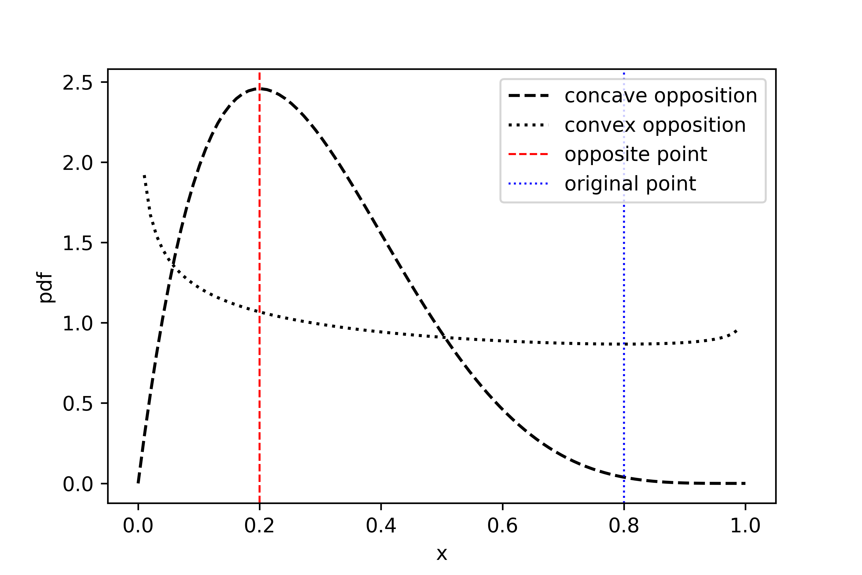
Figure 1: Example of concave and convex opposite points

The following drawbacks affect numerous OBL variants: 1) As OBL variants compute opposite solutions or based on the uniform distribution, there is an inherent limitation in the deterministically search for decent opposite solutions. In other words, there is an opportunity for improvement when computing opposite solutions by using useful probability distributions, such as Cauchy, Gaussian, and $\alpha$-stable ones. 2) When OBL variants compute opposite solutions, the useful elements held with the original solutions can be discarded as all of the elements of the original solutions are transformed into opposites. 3) As OBL variants follow a greedy strategy, fitness evaluations can be wasted if suitable opposite solutions can no longer be discovered at the end of the optimization process.

To overcome these limitations, BetaCOBL uses the following techniques: 1) Beta distribution: BetaCOBL calculates concave or convex opposite solutions by using the beta distribution, which can create various shapes for the continuous probability density functions (PDFs) within the range $[0,1]$. Here, a concave opposite solution represents a solution generated based on a PDF where the opposite point for a given original solution is selected with the highest probability. Conversely, a convex opposite solution is generated based on a PDF where the point for a given original solution is selected with the lowest probability. As a result, with the concave and convex OBLs, BetaCOBL can find appropriate opposite solutions faster than other OBL variants. Fig. 1 shows an example of concave and convex opposite points.

2) Partial dimensional change scheme: BetaCOBL uses the binomial crossover in DE to calculate a partial opposite solution, formed by the recombination of an original solution and its complete opposite solution. Therefore, BetaCOBL can obtain more diverse opposite solutions than other OBL variants as it can have one of the $2^{D}$ possible opposite solutions with a given pair of original and complete opposite solutions. In addition, as it uses the binomial crossover, BetaCOBL can preserve the useful elements held by original solutions.

3) Selection switching scheme: In general, OBL helps discover promising regions at the beginning of an optimization process, but it becomes less effective as the optimization process progresses; as a result, fitness evaluations are potentially wasted. To mitigate this issue, BetaCOBL estimates the population diversity before the concave and convex OBLs. If the population diversity is higher than a predefined threshold $DT$, BetaCOBL uses a $(\mu+\lambda)$ selection with all the original solutions of the population; otherwise, it uses a $(\mu,\lambda)$ selection with the worst half original solutions of the population. Consequently, BetaCOBL can prevent the waste of fitness evaluations by applying one of the two selection operators depending on the convergence progress.

A concave opposite solution is calculated using the beta distribution with both $\alpha$ and $\beta$ greater than one, as follows:

$$\breve{x}_{i,g}^{j}=(x_{max}^{j}-x_{min}^{j})\cdot Beta(\alpha,\beta)+x_{min}^{j}$$ (8)

$$\alpha=\left\{\begin{array}[]{ll}spread\cdot peak&\textrm{if $mode<0.5$}\\ spread&\textrm{otherwise}\end{array}\right.$$ (9)

$$\beta=\left\{\begin{array}[]{ll}spread&\textrm{if $mode<0.5$}\\ spread\cdot peak&\textrm{otherwise}\end{array}\right.$$ (10)

$$spread=\big{(}\frac{1}{\sqrt{normDiv}}\big{)}^{1+N(0,0.5)}$$ (11)

$$peak=\left\{\begin{array}[]{ll}\frac{(spread-2)\cdot mode+1}{spread\cdot(1-mode)}&\textrm{if $mode<0.5$}\\ \frac{2-spread}{spread}+\frac{spread-1}{spread\cdot mode}&\textrm{otherwise}\end{array}\right.$$ (12)

$$mode=\frac{(x_{min}^{j}+x_{max}^{j}-x_{i,g}^{j})-x_{min}^{j}}{x_{max}^{j}-x_{min}^{j}}$$ (13)

where $Beta(\alpha,\beta)$ and $N(0,0.5)$ denote the beta distribution with parameters $\alpha$ and $\beta$, and the Gaussian distribution with the mean $0$ and variance $0.5$, respectively. In addition, the normalized diversity denoted by $normDiv$ is calculated as follows:

$$normDiv=\frac{1}{NP}\sum_{i=1}^{NP}CD(\mathbf{x}_{i,g},\mathbf{P}_{g})$$ (14)

$$CD(\mathbf{x}_{i,g},\mathbf{P}_{g})=\min_{\mathbf{c}\in\mathbf{P}_{g},\mathbf{c}\neq\mathbf{x}_{i,g}}d(\mathbf{c},\mathbf{x}_{i,g})$$ (15)

$$d(\mathbf{c},\mathbf{x}_{i,g})=\sqrt{\frac{1}{D}\sum_{j=1}^{D}\big{(}\frac{x_{i,g}^{j}-c^{j}}{x_{max}^{j}-x_{min}^{j}}\big{)}^{2}}$$ (16)

The same formulas calculate a convex opposite solution except for the mode and spread, calculated as follows:

$$mode=\frac{x_{i,g}^{j}-x_{min}^{j}}{x_{max}^{j}-x_{min}^{j}}$$ (17)

$$spread=0.1\cdot\sqrt{normDiv}+0.9$$ (18)

4.2 Modified Selection Switching Scheme

4.2.1 Problem of Selection Switching Scheme

BetaCOBL uses the selection switching scheme to prevent the waste of fitness evaluations, which applies one of the two selection operators depending on the population diversity. To estimate the population diversity, BetaCOBL calculates the average of the minimum distance between all possible pairs, which is a power mean-based diversity measure. A generalized definition of the power mean-based diversity measure is presented in [15, 16], where it is defined as the mapping $D_{h}:{\rm I\!R}^{NP\times D}\rightarrow{\rm I\!R}$

$$D_{h}(\mathbf{P}_{g},a,b)=\sqrt[b]{\frac{1}{NP}\sum_{i=1}^{NP}d_{i}^{a}}$$ (19)

$$d_{i}^{a}=\frac{1}{NP-1}\sum_{j=1}^{NP}\|\mathbf{x}_{i,g}-\mathbf{x}_{j,g}\|^{a}$$ (20)

where $a,b\neq 0$. The two parameters $a$ and $b$ determine the behavior of the diversity measure. If $a=1$, the arithmetic mean distance of all possible pairs is computed. If $a=0$, the geometric mean distance of all possible pairs is computed. In addition, if $a=-\infty$, the diversity measure evaluates the minimum distance of all possible pairs. Finally, the lower the value of $a$ and $b$, the larger the penalty to the collocation of individuals. The power mean-based diversity measure with $a=-\infty$ and $b=1$ that BetaCOBL uses was experimentally proven not to be $(\rho,\epsilon)$-ectropy where both $\rho$ and $\epsilon$ can simultaneously take values close to zero [69], which means it can discourage the collocation of individuals.

However, the power mean-based diversity measure with $a=-\infty$ and $b=1$ incurs a $O(NP^{2}\cdot D)$ computational cost; as a result it is difficult to use BetaCOBL for optimizing more complex problems with a large population size.

4.2.2 Applying Linear Time Diversity Measure

To reduce the computational cost, we replaced the power mean-based diversity measure with a linear time diversity measure in the selection switching scheme. Of the two well-known measures, we employed one that computes the arithmetic mean of the Euclidean distances of all possible pairs [17, 18, 19, 20, 21, 22, 23, 24, 25], where it can be defined as the mapping $D_{d}:{\rm I\!R}^{NP\times D}\rightarrow{\rm I\!R}$

$$D_{d}(\mathbf{P}_{g})=\frac{1}{2}\sum_{i=1}^{n}\sum_{j=1}^{n}\|\mathbf{x}_{i,g}-\mathbf{x}_{j,g}\|$$ (21)

A naive implementation for equation (21) incurs a $O(NP^{2}\cdot D)$ computational cost. Wineberg and Oppacher [24, 25] reformulated the equation for a linear time diversity measure as follows:

$$D_{d}^{\prime}(\mathbf{P}_{g})=\frac{1}{D}\sqrt{\sum_{k=1}^{D}\overline{(x_{g}^{k})^{2}}-(\overline{x_{g}^{k}})^{2}}$$ (22)

where $\overline{(x_{g}^{k})^{2}}=\frac{1}{NP}\sum_{i=1}^{NP}(x_{i,g}^{k})^{2}$ and $\overline{x_{g}^{k}}=\frac{1}{NP}\sum_{i=1}^{NP}x_{i,g}^{k}$. The computational cost of the reformulated diversity measure is $O(NP\cdot D)$. Note that the proposed algorithm uses the normalized version of the diversity measure, obtained by dividing $\overline{(x_{g}^{k})^{2}}-(\overline{x_{g}^{k}})^{2}$ by $(x_{max}^{k}-x_{min}^{k})$ in the equation (22).

4.2.3 Rationale of Employing Linear Time Diversity Measure

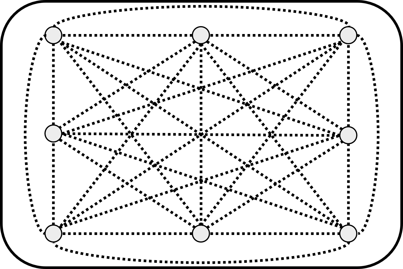
(a) All possible pair

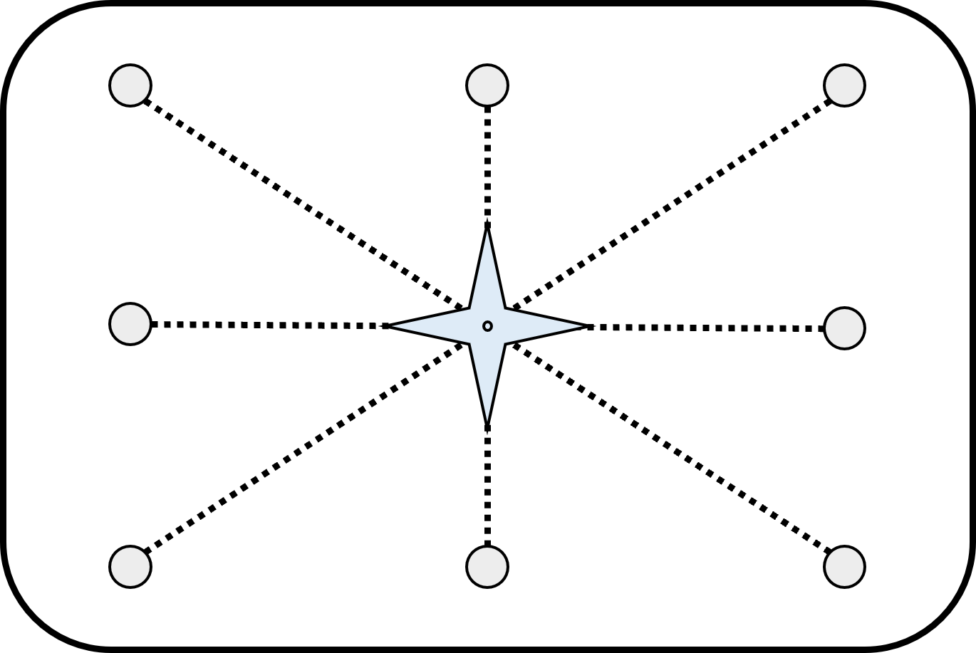
(b) Every point to center point

Figure 2: Two linear time diversity measures

As mentioned in Section 4.2.1, BetaCOBL uses the power mean-based diversity measure to check the convergence progress, which leads to a high computational cost. Therefore, we must replace it with a fast diversity measure to apply BetaCOBL to more complex problems with a large population size.

There are two linear time diversity measures in the multidimensional continuous space. The first measure was discussed in Section 4.2.2 and the other computes the arithmetic mean of the Euclidean distances of every point to the center [70, 71, 72, 73, 21, 22, 23], where it can be defined as the mapping $D_{v}:{\rm I\!R}^{NP\times D}\rightarrow{\rm I\!R}$

$$D_{v}(\mathbf{P}_{g})=\sum_{i=1}^{n}\|\mathbf{x}_{i,g}-\overline{\mathbf{x}}_{g}\|$$ (23)

where $\overline{\mathbf{x}}_{g}=(M^{1},M^{2},\cdots,M^{D})$ and the centroid of the population with $M^{k}=\frac{1}{NP}\sum_{i=1}^{NP}x_{i,g}^{k}$, $k=1,2,\cdots,D$. Fig. 2 shows the two linear time diversity measures.

We chose the first measure as it was theoretically proven to discourage the collocation of individuals bigger than the second measure [69]. Let the population size for each measure be $NP=2^{m}+p$. The ectropic property of the first measure $D_{d}$ is $(\frac{2^{m}}{2^{m}+p},0)$, while that of the second measure $D_{v}$ is $(\frac{1}{2^{m}+p},0)$. Therefore, in a situation where many individuals are in overlapping positions, the second measure is more likely to return a higher value than the first one. In other words, BetaCOBL with the second measure is likely to continue to use the $(\lambda+\mu)$ selection instead of $(\lambda,\mu)$ at the end of the optimization process, which may not prevent the waste of fitness evaluations.

Consequently, the proposed algorithm can estimate the population diversity faster than BetaCOBL with the replacement. In addition, we analyze the relative performance of the original BetaCODE and BetaCODE with the linear time diversity measure and found that there were no significant differences, as reported in Section 6.

4.3 Modified Partial Dimensional Change Scheme

4.3.1 Problem of Partial Dimensional Change Scheme

BetaCOBL uses the binomial crossover in the partial dimensional change scheme to calculate partial opposite solutions. The binomial crossover is the most frequently used crossover operator in DE literature, and has the following properties [74, 26]. First, the relationship between the mutation probability [75] and the control parameter $CR$ is linear. Second, the binomial crossover can generate all the $2^{D}$ possible trial vectors with a given pair of target and mutant vectors. However, it assumes that decision variables are not inter-related; thus, it tends to split up strongly dependent decision variables.

The exponential crossover is the traditional alternative crossover operator; it can preserve adjacent decision variables because of its sequential construct. Although this property helps search for decent solutions on inseparable problems, it has the following critical limitations [74, 26]. First, the control parameter $CR$ is difficult to tune as the relationship between the mutation probability and $CR$ is nonlinear. Second, the exponential crossover cannot generate all of the $2^{D}$ possible trial vectors because of its sequential nature. Therefore, replacing the binomial crossover by the exponential crossover is not only ineffective, but it can also degrade the performance of BetaCOBL.

4.3.2 Applying Multiple Exponential Crossover

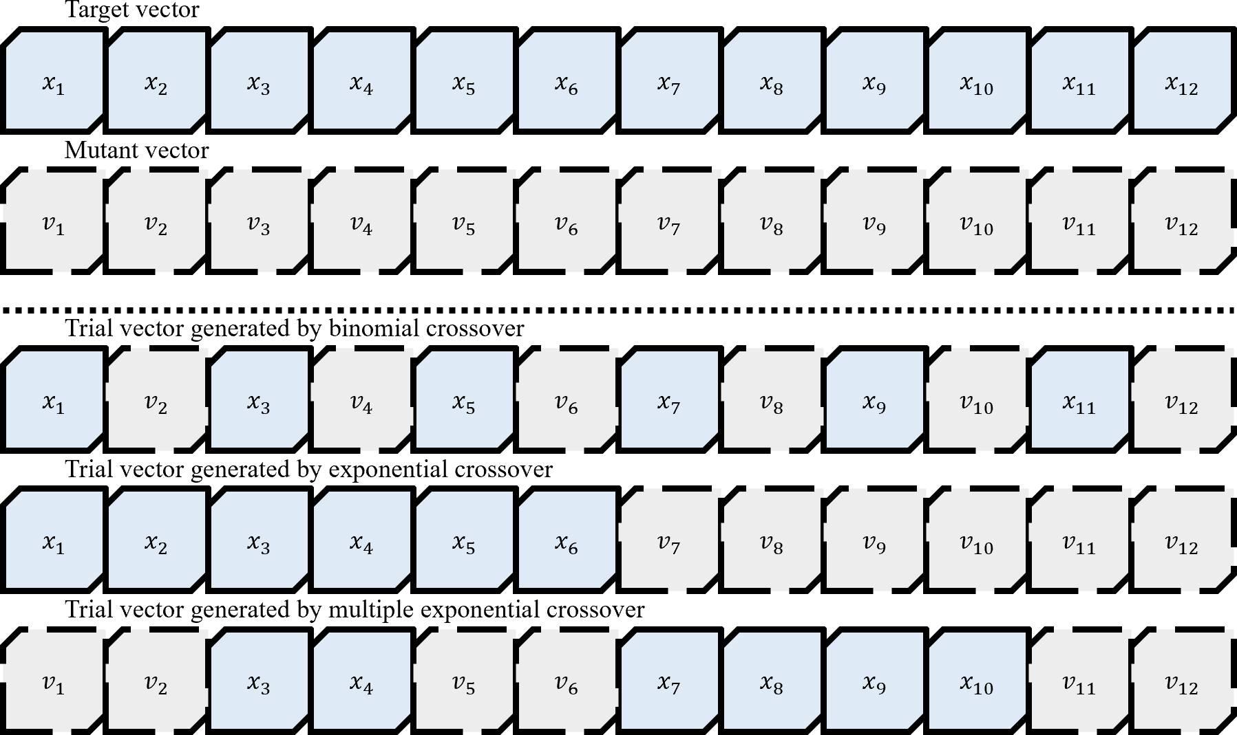
Figure 3: Behavior of three crossover operators

To improve the performance on inseparable problems, we employed the multiple exponential crossover [26] in the partial dimensional change scheme. The multiple exponential crossover is a semi-consecutive crossover operator that divides a trial vector into several components, and each component is a copy of the component at the location of either the target or the mutant vector [26]. Therefore, the multiple exponential crossover is the same as the exponential crossover that is being repeated. Fig. 3 shows the behavior of the binomial, exponential, and multiple exponential crossovers. In the proposed algorithm, the multiple exponential crossover calculates a partial opposite solution with a given pair of target vectors and complete opposite solution as follows. First, an element $n\in[1,D]$ is selected randomly. The four constants, $E_{m}=T\cdot CR$, $E_{s}=T\cdot(1-CR)$, $CR_{m}=\frac{E_{m}}{E_{m}+1}$, and $CR_{s}=\frac{E_{s}}{E_{s}+1}$ are initialized where Em and Es stand for the approximate size of each component copied from the complete opposite solution and the target vector, respectively. Here, the length of the exchanged component $T$ is initialized at ten, as in [26]. Following this, the multiple exponential crossover calculates a partial opposite solution as follows:

1. Starting from the element $n$, a component of Bernoulli trials with $CR_{m}$ is calculated and copied from the complete opposite solution.

2. Starting from the last failure element, the next component of Bernoulli trials with $CR_{s}$ is calculated and copied from the target vector.

3. Repeat from Step 1 until all of the elements are decided.

The pseudo code of the multiple exponential crossover is presented in Algorithm 1.

1

Input : Target vector $\mathbf{x}_{i,g}$, mutant vector $\mathbf{v}_{i,g}$, crossover rate $CR$, and length of exchanged components $T$

Output : Trial vector $\mathbf{u}_{i,g}$

2

3Select random integer $n$ within the range $[1,D]$;

4 $E_{m}=T\cdot CR$, $E_{s}=T\cdot(1-CR)$;

5 $CR_{m}=\frac{E_{m}}{E_{m}+1}$, $CR_{s}=\frac{E_{s}}{E_{s}+1}$;

6 $L=1$, $\textrm{Mutation\_Enable}=1$;

7 repeat

8       if $\textrm{Mutation\_Enable}==1$ then

9             repeat

10                   $u_{i,g}^{\langle n+L-1\rangle_{D}}=v_{i,g}^{\langle n+L-1\rangle_{D}}$;

11                   $L=L+1$;

12                  

13            until $L\leq D$ and $rand_{i,j}\leq CR_{m}$;

14            $\textrm{Mutation\_Enable}=0$;

15            

16      else

17             repeat

18                   $u_{i,g}^{\langle n+L-1\rangle_{D}}=x_{i,g}^{\langle n+L-1\rangle_{D}}$;

19                   $L=L+1$;

20                  

21            until $L\leq D$ and $rand_{i,j}\leq CR_{s}$;

22            $\textrm{Mutation\_Enable}=1$;

23            

24       end if

25      

26until $L\leq D$;

Algorithm 1 Multiple Exponential Crossover

4.3.3 Rationale of Employing Multiple Exponential Crossover

As mentioned in Section 4.3.1, it is of critical importance to preserve strongly dependent decision variables on inseparable problems when searching for satisfactory solutions. However, the exponential crossover is not an alternative to the binomial crossover as tuning the control parameter CR is difficult and it cannot generate all of the possible partial opposite solutions. Using a covariance matrix helps identify the inter-relations between decision variables, but it leads to a high computational cost. Therefore, we employed the multiple exponential crossover, which has the strengths of the exponential crossover but also retains the properties of the binomial crossover. With the replacement, the proposed algorithm can achieve better performance than BetaCOBL on inseparable problems by preserving the strongly dependent decision variables that are adjacent to each other.

4.4 iBetaCODE

iBetaCODE is the combination of DE and iBetaCOBL. As with other ODE variants, iBetaCOBL is executed in the initialization and iteration phases of iBetaCODE. In the initialization phase, iBetaCODE executes iBetaCOBL with the initialized individuals. In the iteration phase, iBetaCODE executes iBetaCOBL or the evolutionary operators of DE alternatively according to a predefined jumping rate $J_{r}$. If a random number generated according to the uniform distribution is lower than or equal to the jumping rate, iBetaCODE performs iBetaCOBL. Otherwise, iBetaCODE executes the evolutionary operators. Regarding the jumping rate, we set $J_{r}=0.05$ in all the experiments in this paper, as in [14]. The entire pseudo code of iBetaCODE is presented in Algorithm 2.

1

Input : Objective function $f(\mathbf{x})$, upper bound $\mathbf{x}_{max}$, lower bound $\mathbf{x}_{min}$, maximum number of function evaluations $NFEs_{max}$, scale factor $F$, crossover rate $CR$, population size $NP$, diversity threshold $DT$, and jumping rate, $J_{r}$

Output : Best objective value $f(\mathbf{x}_{best})$

/* Initialization phase */

2 for $i=0;\ i<NP;\ i=i+1$ do

3       for $j=0;\ j<D;\ j=j+1$ do

4             $x_{i,0}^{j}=x_{min}^{j}+rand_{i}^{j}\cdot(x_{max}^{j}-x_{min}^{j})$;

5            

6       end for

7      

8 end for

9$NFEs=NP,g=1$;

10 Calculate $normDiv$ using equation (22);

11 if $normDiv>DT$ then

12       $(\mu+\lambda)$ selection phase of iBetaCOBL (Algorithm 3);

13      

14else

15       $(\mu,\lambda)$ selection phase of iBetaCOBL (Algorithm 4);

16      

17 end if

/* Iteration phase */

18 while None of termination criteria is satisfied do

19       for $i=0;\ i<NP;\ i=i+1$ do

20             if $rand_{i}\leq J_{r}$ then

21                   Calculate $normDiv$ using equation (22);

22                   if $normDiv>DT$ then

23                         $(\mu+\lambda)$ selection phase of iBetaCOBL (Algorithm 3);

24                        

25                  else

26                         $(\mu,\lambda)$ selection phase of iBetaCOBL (Algorithm 4);

27                        

28                   end if

29                  

30            else

31                   Select random three donor vectors $\mathbf{x}_{r_{1},g}$, $\mathbf{x}_{r_{2},g}$, $\mathbf{x}_{r_{3},g}$ where $r_{1}\neq r_{2}\neq r_{3}\neq i$;

32                   Select random integer $j_{rand}$ within the range $[1,D]$;

33                   for $j=0;\ j<D;\ j=j+1$ do

34                         if $rand_{i}^{j}\leq CR$ or $j=j_{rand}$ then

35                               $u_{i,g}^{j}=x_{r_{1},g}^{j}+F\cdot(x_{r_{2},g}^{j}-x_{r_{3},g}^{j})$;

36                              

37                        else

38                               $u_{i,g}^{j}=x_{i,g}^{j}$;

39                              

40                         end if

41                        

42                   end for

43                  for $i=0;\ i<NP;\ i=i+1$ do

44                         if $f(\mathbf{u}_{i,g})\leq f(\mathbf{x}_{i,g})$ then

45                               $\mathbf{x}_{i,g+1}=\mathbf{u}_{i,g}$;

46                              

47                        else

48                               $\mathbf{x}_{i,g+1}=\mathbf{x}_{i,g}$;

49                              

50                         end if

51                        

52                   end for

53                  $NFEs=NFEs+NP$;

54                  

55             end if

56            

57       end for

58      $g=g+1$;

59      

60 end while

Algorithm 2 iBetaCODE

1

Input : Population $\mathbf{P}_{g}$

Output : Population $\mathbf{P}_{g}^{\prime}$

2

/* $(\mu+\lambda)$ selection */

3 Set opposite population $\mathbf{OP}_{g}=(\mathbf{\breve{x}}_{1,g},\mathbf{\breve{x}}_{2,g},\cdots,\mathbf{\breve{x}}_{NP\cdot 2,g})$;

4 for $i=0;\ i<NP;\ i=i+1$ do

5       if $rand_{i}\leq 0.5$ then

6             Calculate spread using equation (11);

7             for $j=0;\ j<D;\ j=j+1$ do

8                   Calculate mode using equation (13);

9                   Calculate peak using equation (12);

10                   Calculate alpha using equation (9);

11                   Calculate beta using equation (10);

12                   $t_{i,g}^{j}=(x_{max}^{j}-x_{min}^{j})\cdot Beta(\alpha,\beta)+x_{min}^{j}$;

13                  

14             end for

15            

16      else

17             Calculate spread using equation (18);

18             for $j=0;\ j<D;\ j=j+1$ do

19                   Calculate mode using equation (17);

20                   Calculate peak using equation (12);

21                   Calculate alpha using equation (9);

22                   Calculate beta using equation (10);

23                   $t_{i,g}^{j}=(x_{max}^{j}-x_{min}^{j})\cdot Beta(\alpha,\beta)+x_{min}^{j}$;

24                  

25             end for

26            

27       end if

28      Calculate a partial opposite solution $\mathbf{\breve{x}}_{i,g}$ using Algorithm 1 with $\mathbf{t}_{i,g}$, $\mathbf{x}_{i,g}$, and $CR=0.1$;

29       Calculate a partial opposite solution $\mathbf{\breve{x}}_{i+NP,g}$ using Algorithm 1 with $\mathbf{t}_{i,g}$, $\mathbf{x}_{i,g}$, and $CR=0.9$;

30      

31 end for

32Merge original and opposite populations $\mathbf{P}_{g}+\mathbf{OP}_{g}$;

33 Select $NP$ best individuals $\mathbf{P}_{g}^{\prime}$ from merged population $\mathbf{P}_{g}+\mathbf{OP}_{g}$;

34 $NFEs=NFEs+(NP\cdot 2)$;

35

Algorithm 3 $(\mu+\lambda)$ Selection Phase of iBetaCOBL

1

Input : Population $\mathbf{P}_{g}$

Output : Population $\mathbf{P}_{g}^{\prime}$

2

/* $(\mu,\lambda)$ selection */

3 Sort population $\mathbf{P}_{g}$;

4 for $i=\frac{NP}{2};\ i<NP;\ i=i+1$ do

5       if $rand_{i}\leq 0.5$ then

6             Calculate spread using equation (11);

7             for $j=0;\ j<D;\ j=j+1$ do

8                   Calculate mode using equation (13);

9                   Calculate peak using equation (12);

10                   Calculate alpha using equation (9);

11                   Calculate beta using equation (10);

12                   $t_{i,g}^{j}=(x_{max}^{j}-x_{min}^{j})\cdot Beta(\alpha,\beta)+x_{min}^{j}$;

13                  

14             end for

15            

16      else

17             Calculate spread using equation (18);

18             for $j=0;\ j<D;\ j=j+1$ do

19                   Calculate mode using equation (17);

20                   Calculate peak using equation (12);

21                   Calculate alpha using equation (9);

22                   Calculate beta using equation (10);

23                   $t_{i,g}^{j}=(x_{max}^{j}-x_{min}^{j})\cdot Beta(\alpha,\beta)+x_{min}^{j}$;

24                  

25             end for

26            

27       end if

28      Calculate a partial opposite solution $\mathbf{\breve{x}}_{1,g}$ using Algorithm 1 with $\mathbf{t}_{i,g}$, $\mathbf{x}_{i,g}$, and $CR=0.1$;

29       Calculate a partial opposite solution $\mathbf{\breve{x}}_{2,g}$ using Algorithm 1 with $\mathbf{t}_{i,g}$, $\mathbf{x}_{i,g}$, and $CR=0.9$;

30       if $f(\mathbf{\breve{x}}_{1,g})\leq f(\mathbf{\breve{x}}_{2,g})$ then

31             if $f(\mathbf{\breve{x}}_{1,g})\leq f(\mathbf{x}_{i,g})$ then

32                   $\mathbf{x}_{i,g}=\mathbf{\breve{x}}_{1,g}$;

33                  

34             end if

35            

36      else

37             if $f(\mathbf{\breve{x}}_{2,g})\leq f(\mathbf{x}_{i,g})$ then

38                   $\mathbf{x}_{i,g}=\mathbf{\breve{x}}_{2,g}$;

39                  

40             end if

41            

42       end if

43      

44 end for

45$NFEs=NFEs+NP$;

46

Algorithm 4 $(\mu,\lambda)$ Selection Phase of iBetaCOBL

5 Experimental Setup

All the experiments were conducted on Windows 10 Pro 64 bit of a PC with AMD Ryzen Threadripper 2990WX @ 3.0GHz. All the test algorithms were implemented in the C++ programming language with Visual Studio 2019 64 bit.

5.1 Test Functions

We utilized a set of 58 test functions for demonstrating the performance of the proposed algorithm. There are four well-known test suites on single objective bound constrained real-parameter numerical optimization, such as the CEC 2005, 2013, 2014, and 2017 test suites. We chose the CEC 2013 and 2017 test suites because the former is a directly improved version of the CEC 2005 test suite, while the latter is a directly improved version of the CEC 2014 test suite. In the CEC 2013 test suite, there are five unimodal functions ($F_{1}$-$F_{5}$), fifteen simple multimodal functions ($F_{6}$-$F_{20}$), and eight composition functions ($F_{21}$-$F_{28}$). In the CEC 2017 test suite, there are three unimodal functions ($F_{1}$-$F_{3}$), seven simple multimodal functions ($F_{4}$-$F_{10}$), ten expanded multimodal functions ($F_{11}$-$F_{20}$), and ten hybrid composition functions ($F_{21}$-$F_{30}$). For more detail explanations of the CEC 2013 and 2017 test suites, please refer to the following technical reports [27, 28].

The experimental settings, such as the number of runs, the maximum number of function evaluations, and the minimum and maximum bounds, are initialized in the same way as in [27] and [28].

5.2 Performance Metrics

5.2.1 Function Error Value

We utilized function error value (FEV) to evaluate the accuracy of a test algorithm, which can be defined as follows.

$$\textrm{FEV}=f(\mathbf{x}_{best,g_{max}})-f(\mathbf{x}_{*})$$ (24)

where $f(x)$ stands for an objective function to be minimized. Also, $\mathbf{x}_{best,g_{max}}$ is the best solution found by a test algorithm, and $\mathbf{x}_{*}$ is the global optimum of a given problem. The lower the value of FEV, the higher the accuracy of a test algorithm.

5.2.2 Statistical Test

To determine whether the difference in performance for two test algorithms is significant or not, we utilized the Wilcoxon rank-sum test with $\alpha=0.05$ significance level [76]. The symbols in this paper have the following meanings unless stated otherwise.

1. +: The corresponding algorithm finds significantly better solutions than the proposed algorithm.

2. =: The performance difference between the proposed algorithm and the corresponding algorithm is not statistically significant.

3. -: The corresponding algorithm finds significantly worse solutions than the proposed algorithm.

Also, to determine whether the difference in performance for multiple test algorithms is significant or not, we utilized the Friedman test with Hochberg’s post hoc [76].

6 Results and Comparisons

6.1 Comparison with Ten OBL Variants

We performed experiments to evaluate the performance of iBetaCOBL and compared it to ten state-of-the-art OBL variants, namely: 1) OBL [13], 2) OBLTVJR [61], 3) OBLPGJ [62], 4) QOBL [63], 5) QROBL [64], 6) COOBL [65], 7) GOBL [66], 8) EOBL [67], 9) AGOBL [68], and 10) BetaCOBL [14]. For a fair comparison, we used the same classical DE variant called DE/rand/1/bin; regarding the control parameters associated with the DE variant, we used the following values: $F=0.5$, $CR=0.9$, and $NP=100$. Additionally, we used the values recommended by the authors of each paper for the remaining control parameters.

6.1.1 Performance Evaluation on CEC 2013 Test Suite

In this subsection, the performance evaluation results on the CEC 2013 test suite are presented. Twenty-eight benchmark problems from the CEC 2013 test suite are utilized to evaluate the performance of the test algorithms. Both 30-$D$ and 50-$D$ versions of the benchmark problems are tested.

Table 1 shows the averages and standard deviations of the FEVs of each algorithm at 30 dimension, collected through 51 independent runs. As we can see from the table, the proposed algorithm has a clear edge over all the other OBL variants. More specifically, iBetaCOBL found more significantly accurate solutions than COOBL, OBL, OBLTVJR, QOBL, and QROBL on more than half of the test functions. In particular, iBetaCOBL considerably outperformed COOBL and QROBL on approximately four-fifths of the test functions. The second and third best algorithms are BetaCOBL and OBLPGJ, respectively. Compared with the original DE/rand/1/bin, DE/rand/1/bin assisted by iBetaCOBL considerably outperformed it on 12 test functions and underperformed it on 5 test functions. Compared with BetaCOBL, iBetaCOBL considerably outperformed it on 12 test functions and underperformed it on 6 test functions. In a word, DE/rand/1/bin assisted by iBetaCOBL secures an overall better performance than all the other OBL variants.

Also, Table 2 shows the Friedman test with Hochberg’s post hoc, which supports the experimental results in Table 1 where iBetaCOBL ranked the first among the test algorithms, and the outperformance over COOBL, EOBL, OBL, OBLTVJR, and QROBL was statistically significant. In summary, the proposed algorithm is superior to the test algorithms on the CEC 2013 test suite at 30 dimension.

Additionally, we analyzed the performance evaluation results in Table 1 based on the attributes of the test functions. The proposed algorithm achieved a similar optimization performance comparatively on the unimodal functions ($F_{1}$-$F_{5}$). However, it achieved a significantly better optimization performance in solving the multimodal ($F_{6}$-$F_{20}$) and composition functions ($F_{21}$-$F_{28}$). The results revealed that the proposed algorithm has a strong exploration property, and is thus capable of discovering more satisfactory solutions comparatively for more complex test functions.

We found similar tendencies at 50 dimension in Tables 3 and 4. Compared with the experimental results at 30 dimension, the outperformance of the proposed algorithm is slightly larger at 50 dimension. For example, iBetaCOBL found more significantly accurate solutions on more than half the test functions compared with all the test algorithms except BetaCOBL. In particular, iBetaCOBL considerably outperformed COOBL, QOBL, and QROBL on approximately four-fifths of the test functions. Therefore, the proposed algorithm demonstrates that it can achieve better searchability than all the compared ones, including its predecessor BetaCOBL, particularly in the optimization for the multimodal and composition functions of the CEC 2013 test suite at both 30 and 50 dimensions.

Table 1: Averages and standard deviations of FEVs of DE/rand/1/bin with OBL variants on CEC 2013 test suite at 30-$D$.

	DE/rand/1/bin
	iBetaCOBL	Original	AGOBL	BetaCOBL	COOBL	EOBL	GOBL
	MEAN (STD DEV)	MEAN (STD DEV)	MEAN (STD DEV)	MEAN (STD DEV)	MEAN (STD DEV)	MEAN (STD DEV)	MEAN (STD DEV)
F1	0.00E+00 (0.00E+00)	0.00E+00 (0.00E+00) =	0.00E+00 (0.00E+00) =	0.00E+00 (0.00E+00) =	0.00E+00 (0.00E+00) =	0.00E+00 (0.00E+00) =	0.00E+00 (0.00E+00) =
F2	4.01E+05 (2.25E+05)	3.71E+05 (2.96E+05) =	4.77E+05 (2.96E+05) =	4.86E+05 (3.34E+05) =	1.50E+05 (9.22E+04) +	4.55E+05 (2.79E+05) =	5.95E+05 (4.86E+05) =
F3	1.69E+03 (1.11E+04)	7.30E-01 (4.09E+00) +	2.75E+04 (1.95E+05) =	1.74E+02 (9.14E+02) =	1.42E+08 (9.67E+08) -	5.18E+00 (2.77E+01) +	3.90E+00 (1.60E+01) =
F4	1.06E+03 (6.81E+02)	9.68E+02 (4.64E+02) =	1.13E+03 (6.27E+02) =	1.38E+03 (5.49E+02) -	1.61E+04 (3.04E+04) -	2.87E+04 (1.07E+05) -	1.05E+03 (4.58E+02) =
F5	9.39E-14 (4.39E-14)	8.72E-14 (4.88E-14) =	8.94E-14 (4.74E-14) =	9.16E-14 (4.57E-14) =	7.82E-14 (5.34E-14) =	9.16E-14 (4.57E-14) =	7.60E-14 (5.43E-14) =
F6	1.20E+01 (5.70E+00)	8.69E+00 (3.17E+00) +	1.17E+01 (5.48E+00) +	1.06E+01 (6.38E+00) +	1.72E+01 (1.66E+01) -	1.04E+01 (5.38E+00) +	1.03E+01 (5.52E+00) +
F7	4.04E-01 (5.61E-01)	2.06E-01 (3.15E-01) =	1.78E-01 (1.99E-01) =	1.38E-01 (2.01E-01) +	5.56E+01 (3.38E+01) -	1.42E-01 (2.15E-01) +	1.20E-01 (1.58E-01) +
F8	2.10E+01 (7.17E-02)	2.10E+01 (5.79E-02) +	2.09E+01 (6.74E-02) +	2.10E+01 (5.77E-02) +	2.11E+01 (8.65E-02) -	2.10E+01 (6.42E-02) =	2.10E+01 (6.12E-02) +
F9	1.03E+01 (4.56E+00)	2.54E+01 (1.45E+01) -	7.73E+00 (2.77E+00) +	6.46E+00 (2.28E+00) +	3.18E+01 (1.12E+01) -	1.84E+01 (1.43E+01) =	9.13E+00 (7.03E+00) +
F10	1.13E-02 (7.88E-03)	6.96E-03 (7.54E-03) +	7.15E-03 (6.83E-03) +	6.67E-03 (5.58E-03) +	3.62E-02 (1.82E-02) -	7.97E-03 (7.78E-03) +	5.17E-03 (5.22E-03) +
F11	1.38E+01 (4.27E+00)	1.30E+02 (2.53E+01) -	1.38E+02 (2.12E+01) -	4.78E+01 (1.04E+01) -	7.47E+01 (3.57E+01) -	1.30E+02 (2.70E+01) -	1.39E+02 (2.43E+01) -
F12	4.73E+01 (2.25E+01)	1.80E+02 (1.09E+01) -	1.82E+02 (1.01E+01) -	1.74E+02 (1.13E+01) -	1.76E+02 (5.85E+01) -	1.78E+02 (2.45E+01) -	1.81E+02 (1.02E+01) -
F13	7.41E+01 (2.57E+01)	1.79E+02 (1.18E+01) -	1.82E+02 (1.02E+01) -	1.76E+02 (1.19E+01) -	1.91E+02 (5.45E+01) -	1.77E+02 (1.94E+01) -	1.80E+02 (1.15E+01) -
F14	2.71E+02 (1.16E+02)	6.27E+03 (4.81E+02) -	4.44E+03 (6.50E+02) -	1.11E+03 (2.80E+02) -	3.41E+03 (8.94E+02) -	5.77E+03 (1.09E+03) -	5.08E+03 (1.02E+03) -
F15	5.16E+03 (8.39E+02)	7.06E+03 (2.77E+02) -	3.98E+03 (1.57E+03) +	7.06E+03 (2.84E+02) -	8.06E+03 (6.11E+02) -	6.97E+03 (5.41E+02) -	6.30E+03 (1.61E+03) -
F16	2.44E+00 (4.05E-01)	2.42E+00 (2.92E-01) =	2.34E+00 (5.20E-01) =	2.50E+00 (2.39E-01) =	3.87E+00 (4.66E-01) -	2.48E+00 (2.82E-01) =	2.47E+00 (2.76E-01) =
F17	5.06E+01 (5.02E+00)	1.85E+02 (1.51E+01) -	1.86E+02 (1.68E+01) -	1.03E+02 (1.19E+01) -	1.23E+02 (2.80E+01) -	2.33E+02 (3.37E+02) -	1.86E+02 (1.61E+01) -
F18	1.52E+02 (3.33E+01)	2.08E+02 (1.06E+01) -	2.14E+02 (1.12E+01) -	2.08E+02 (1.01E+01) -	2.45E+02 (3.68E+01) -	2.32E+02 (1.26E+02) -	2.12E+02 (9.92E+00) -
F19	2.75E+00 (6.58E-01)	1.50E+01 (1.14E+00) -	1.51E+01 (1.22E+00) -	1.14E+01 (1.46E+00) -	8.41E+00 (3.00E+00) -	6.72E+01 (3.73E+02) -	1.53E+01 (1.02E+00) -
F20	1.11E+01 (7.69E-01)	1.20E+01 (2.90E-01) -	1.21E+01 (2.70E-01) -	1.22E+01 (2.21E-01) -	1.31E+01 (6.99E-01) -	1.21E+01 (2.62E-01) -	1.21E+01 (2.45E-01) -
F21	2.89E+02 (8.96E+01)	3.10E+02 (9.33E+01) =	3.33E+02 (9.79E+01) -	3.15E+02 (8.58E+01) =	3.10E+02 (8.52E+01) =	4.49E+02 (6.63E+02) =	3.14E+02 (9.06E+01) =
F22	3.39E+02 (1.06E+02)	6.19E+03 (5.61E+02) -	4.80E+03 (8.68E+02) -	1.07E+03 (2.50E+02) -	3.57E+03 (1.33E+03) -	6.25E+03 (8.82E+02) -	5.48E+03 (9.84E+02) -
F23	4.68E+03 (8.97E+02)	7.04E+03 (2.66E+02) -	5.16E+03 (1.74E+03) =	6.93E+03 (3.44E+02) -	8.38E+03 (8.28E+02) -	7.11E+03 (5.33E+02) -	6.80E+03 (8.85E+02) -
F24	2.00E+02 (1.83E+00)	2.00E+02 (0.00E+00) =	2.00E+02 (0.00E+00) =	2.00E+02 (0.00E+00) =	2.29E+02 (2.02E+01) -	2.00E+02 (0.00E+00) =	2.00E+02 (0.00E+00) =
F25	2.41E+02 (3.96E+00)	2.40E+02 (4.53E+00) =	2.39E+02 (4.87E+00) +	2.40E+02 (4.75E+00) =	2.80E+02 (2.34E+01) -	2.39E+02 (4.81E+00) +	2.41E+02 (4.52E+00) =
F26	2.00E+02 (0.00E+00)	2.02E+02 (1.40E+01) =	2.00E+02 (0.00E+00) =	2.00E+02 (0.00E+00) =	2.18E+02 (5.10E+01) =	2.04E+02 (2.13E+01) =	2.00E+02 (0.00E+00) =
F27	3.18E+02 (5.08E+01)	3.11E+02 (4.09E+01) +	3.12E+02 (3.96E+01) =	3.04E+02 (1.91E+01) +	8.48E+02 (2.78E+02) -	3.11E+02 (4.06E+01) =	3.04E+02 (2.16E+01) +
F28	3.00E+02 (0.00E+00)	3.00E+02 (0.00E+00) =	3.00E+02 (0.00E+00) =	3.00E+02 (0.00E+00) =	3.23E+02 (1.65E+02) =	3.00E+02 (0.00E+00) =	3.00E+02 (0.00E+00) =
+/=/-		5/11/12	6/12/10	6/10/12	1/5/22	5/11/12	6/11/11
			OBL	OBLPGJ	OBLTVJR	QOBL	QROBL
			MEAN (STD DEV)	MEAN (STD DEV)	MEAN (STD DEV)	MEAN (STD DEV)	MEAN (STD DEV)
F1			0.00E+00 (0.00E+00) =	0.00E+00 (0.00E+00) =	0.00E+00 (0.00E+00) =	0.00E+00 (0.00E+00) =	2.46E+02 (3.40E+02) -
F2			7.18E+05 (4.75E+05) -	4.43E+05 (3.74E+05) =	5.47E+05 (3.36E+05) -	3.81E+05 (2.65E+05) =	8.21E+06 (2.33E+06) -
F3			2.80E+01 (1.71E+02) -	3.97E-01 (1.96E+00) +	6.14E+04 (4.38E+05) -	3.68E+05 (7.26E+05) -	2.65E+09 (2.96E+09) -
F4			2.42E+03 (9.40E+02) -	9.54E+02 (4.51E+02) =	2.32E+03 (9.57E+02) -	4.22E+02 (2.02E+02) +	9.43E+03 (3.45E+03) -
F5			9.84E-14 (3.96E-14) =	8.27E-14 (5.14E-14) =	1.05E-13 (3.10E-14) =	8.57E-04 (3.93E-03) =	4.41E+02 (6.27E+02) -
F6			1.25E+01 (9.32E+00) =	8.67E+00 (4.24E+00) +	1.06E+01 (2.52E+00) =	2.17E+01 (1.77E+01) -	9.44E+01 (3.16E+01) -
F7			3.35E-01 (3.69E-01) =	1.07E-01 (2.14E-01) +	2.74E-01 (3.23E-01) =	5.88E-01 (9.56E-01) =	8.07E+01 (2.19E+01) -
F8			2.10E+01 (6.88E-02) =	2.10E+01 (6.59E-02) =	2.10E+01 (8.17E-02) =	2.09E+01 (5.78E-02) +	2.10E+01 (5.04E-02) +
F9			1.31E+01 (9.22E+00) =	1.52E+01 (1.17E+01) =	1.35E+01 (9.12E+00) =	1.68E+01 (1.43E+01) =	2.33E+01 (3.19E+00) -
F10			7.49E-03 (7.80E-03) +	5.65E-03 (5.03E-03) +	6.28E-03 (6.74E-03) +	1.17E-01 (8.92E-02) -	2.66E+01 (2.32E+01) -
F11			1.53E+02 (1.82E+01) -	1.27E+02 (2.57E+01) -	1.52E+02 (2.06E+01) -	6.15E+01 (2.72E+01) -	1.78E+02 (6.39E+01) -
F12			1.82E+02 (1.02E+01) -	1.79E+02 (9.07E+00) -	1.83E+02 (8.25E+00) -	1.33E+02 (4.81E+01) -	1.68E+02 (5.54E+01) -
F13			1.83E+02 (8.54E+00) -	1.80E+02 (1.06E+01) -	1.81E+02 (1.05E+01) -	1.42E+02 (4.19E+01) -	2.45E+02 (5.33E+01) -
F14			4.11E+03 (7.87E+02) -	4.23E+03 (8.47E+02) -	4.07E+03 (8.27E+02) -	6.42E+03 (4.57E+02) -	2.33E+03 (6.81E+02) -
F15			6.20E+03 (1.26E+03) -	6.57E+03 (1.02E+03) -	6.24E+03 (9.78E+02) -	7.09E+03 (2.58E+02) -	4.03E+03 (6.51E+02) +
F16			2.48E+00 (6.02E-01) =	2.56E+00 (4.79E-01) =	2.68E+00 (6.30E-01) -	2.46E+00 (2.55E-01) =	2.35E+00 (4.79E-01) =
F17			1.97E+02 (1.33E+01) -	1.82E+02 (1.56E+01) -	1.93E+02 (1.65E+01) -	1.67E+02 (1.55E+01) -	1.93E+02 (5.52E+01) -
F18			2.14E+02 (1.18E+01) -	2.09E+02 (1.23E+01) -	2.13E+02 (1.16E+01) -	1.89E+02 (1.11E+01) -	1.46E+02 (3.86E+01) =
F19			1.52E+01 (9.52E-01) -	1.50E+01 (1.03E+00) -	1.53E+01 (8.88E-01) -	1.27E+01 (1.46E+00) -	5.55E+02 (2.56E+03) -
F20			1.22E+01 (3.27E-01) -	1.20E+01 (4.02E-01) -	1.23E+01 (1.96E-01) -	1.19E+01 (3.04E-01) -	1.11E+01 (8.54E-01) =
F21			3.02E+02 (8.69E+01) =	3.19E+02 (9.09E+01) =	3.25E+02 (9.70E+01) =	3.38E+02 (8.10E+01) -	5.69E+02 (2.01E+02) -
F22			4.28E+03 (7.62E+02) -	4.47E+03 (8.91E+02) -	4.31E+03 (8.73E+02) -	6.37E+03 (5.71E+02) -	2.61E+03 (7.62E+02) -
F23			6.42E+03 (1.16E+03) -	6.64E+03 (1.13E+03) -	6.29E+03 (1.52E+03) -	7.04E+03 (3.02E+02) -	5.04E+03 (1.05E+03) =
F24			2.00E+02 (0.00E+00) =	2.00E+02 (0.00E+00) =	2.00E+02 (3.11E-01) =	2.02E+02 (2.72E+00) -	2.62E+02 (1.31E+01) -
F25			2.41E+02 (4.57E+00) =	2.40E+02 (4.49E+00) =	2.41E+02 (4.48E+00) =	2.39E+02 (7.28E+00) =	2.89E+02 (1.13E+01) -
F26			2.04E+02 (1.97E+01) =	2.00E+02 (0.00E+00) =	2.02E+02 (1.40E+01) =	2.02E+02 (1.46E+01) =	2.23E+02 (5.30E+01) -
F27			3.12E+02 (3.40E+01) =	3.10E+02 (4.52E+01) +	3.16E+02 (5.17E+01) =	3.34E+02 (3.06E+01) -	8.57E+02 (1.07E+02) -
F28			3.00E+02 (0.00E+00) =	3.00E+02 (0.00E+00) =	3.00E+02 (0.00E+00) =	2.96E+02 (2.80E+01) =	1.42E+03 (7.23E+02) -
+/=/-			1/13/14	5/12/11	1/12/15	2/9/17	2/4/22

The symbols “+/=/-” indicate that DE/rand/1/bin with a given OBL performed significantly better ($+$), not significantly better or worse ($=$), or significantly worse ($-$) compared to DE/rand/1/bin with iBetaCOBL using the Wilcoxon rank-sum test with $\alpha=0.05$ significance level.

Table 2: Friedman test with Hochberg’s post hoc for DE/rand/1/bin with OBL variants on CEC 2013 test suite at 30-$D$.

	DE/rand/1/bin
	Algorithm	Average ranking	z-value	p-value	Adj. p-value (Hochberg)	Sig.		Test statistics
1	iBetaCOBL	4.54
2	Original	5.63	-1.13.E+00	2.58.E-01	7.75.E-01	No		N	28
3	AGOBL	5.88	-1.39.E+00	1.65.E-01	8.23.E-01	No		Chi-Square	50.25
4	BetaCOBL	4.80	-2.78.E-01	7.81.E-01	7.81.E-01	No		df	11
5	COOBL	8.50	-4.11.E+00	3.89.E-05	3.89.E-04	Yes		p-value	5.65.E-07
6	EOBL	7.38	-2.95.E+00	3.21.E-03	2.25.E-02	Yes		Sig.	Yes
7	GOBL	5.64	-1.15.E+00	2.51.E-01	1.00.E+00	No
8	OBL	7.66	-3.24.E+00	1.18.E-03	9.46.E-03	Yes
9	OBLPGJ	5.00	-4.82.E-01	6.30.E-01	1.26.E+00	No
10	OBLTVJR	7.70	-3.28.E+00	1.04.E-03	9.34.E-03	Yes
11	QOBL	6.57	-2.11.E+00	3.46.E-02	2.08.E-01	No
12	QROBL	8.71	-4.34.E+00	1.45.E-05	1.59.E-04	Yes

Table 3: Averages and standard deviations of FEVs of DE/rand/1/bin with OBL variants on CEC 2013 test suite at 50-$D$.

	DE/rand/1/bin
	iBetaCOBL	Original	AGOBL	BetaCOBL	COOBL	EOBL	GOBL
	MEAN (STD DEV)	MEAN (STD DEV)	MEAN (STD DEV)	MEAN (STD DEV)	MEAN (STD DEV)	MEAN (STD DEV)	MEAN (STD DEV)
F1	4.45E-15 (3.18E-14)	0.00E+00 (0.00E+00) =	1.78E-14 (6.16E-14) =	1.34E-14 (5.39E-14) =	0.00E+00 (0.00E+00) =	4.45E-15 (3.18E-14) =	0.00E+00 (0.00E+00) =
F2	1.48E+06 (6.36E+05)	2.99E+06 (1.04E+06) -	4.22E+06 (1.79E+06) -	3.09E+06 (1.34E+06) -	6.10E+05 (1.90E+05) +	3.10E+06 (1.07E+06) -	3.08E+06 (9.96E+05) -
F3	5.97E+05 (1.29E+06)	4.18E+05 (8.58E+05) =	3.01E+05 (4.88E+05) =	7.69E+05 (1.21E+06) =	1.03E+09 (4.05E+09) -	4.73E+05 (1.01E+06) =	2.20E+05 (2.97E+05) =
F4	6.22E+03 (1.59E+03)	1.82E+04 (3.64E+03) -	2.37E+04 (4.99E+03) -	2.00E+04 (3.74E+03) -	6.02E+04 (4.83E+04) -	2.09E+04 (5.30E+03) -	2.15E+04 (4.12E+03) -
F5	1.12E-13 (1.60E-14)	1.12E-13 (1.60E-14) =	1.14E-13 (7.65E-29) =	1.14E-13 (7.65E-29) =	1.12E-13 (1.60E-14) =	1.80E+02 (9.58E+02) =	1.14E-13 (7.65E-29) =
F6	4.34E+01 (8.91E-02)	4.35E+01 (8.16E-01) =	4.34E+01 (1.40E-02) =	4.34E+01 (1.82E-01) =	4.38E+01 (1.39E+00) =	7.25E+02 (4.87E+03) =	4.34E+01 (2.38E-02) =
F7	2.35E+00 (2.04E+00)	1.88E+00 (2.15E+00) =	1.81E+00 (1.74E+00) =	1.59E+00 (1.62E+00) +	1.05E+02 (3.55E+01) -	2.16E+00 (2.22E+00) =	1.28E+00 (1.42E+00) +
F8	2.12E+01 (5.04E-02)	2.11E+01 (4.78E-02) +	2.11E+01 (4.69E-02) =	2.11E+01 (5.32E-02) =	2.13E+01 (4.31E-02) -	2.11E+01 (4.83E-02) +	2.11E+01 (5.47E-02) =
F9	1.94E+01 (7.62E+00)	6.73E+01 (1.24E+01) -	1.74E+01 (5.84E+00) =	1.45E+01 (3.99E+00) +	6.94E+01 (1.32E+01) -	4.26E+01 (2.76E+01) -	2.20E+01 (1.79E+01) =
F10	3.87E-02 (2.44E-02)	2.97E-02 (1.49E-02) =	3.94E-02 (2.03E-02) =	3.62E-02 (2.03E-02) =	7.92E-02 (3.71E-02) -	3.83E-02 (1.85E-02) =	3.43E-02 (1.50E-02) =
F11	3.00E+01 (7.24E+00)	1.86E+02 (4.08E+01) -	2.19E+02 (4.09E+01) -	1.10E+02 (2.64E+01) -	1.43E+02 (6.36E+01) -	2.28E+02 (2.32E+02) -	2.12E+02 (4.82E+01) -
F12	7.34E+01 (3.59E+01)	3.56E+02 (1.37E+01) -	3.60E+02 (1.32E+01) -	3.51E+02 (1.44E+01) -	3.18E+02 (1.32E+02) -	3.55E+02 (4.91E+01) -	3.60E+02 (1.17E+01) -
F13	1.28E+02 (3.62E+01)	3.56E+02 (1.30E+01) -	3.56E+02 (1.65E+01) -	3.58E+02 (1.36E+01) -	4.07E+02 (7.00E+01) -	3.58E+02 (1.36E+01) -	3.54E+02 (1.36E+01) -
F14	7.16E+02 (1.73E+02)	1.13E+04 (1.19E+03) -	8.53E+03 (9.29E+02) -	2.97E+03 (4.32E+02) -	7.12E+03 (1.45E+03) -	1.02E+04 (1.57E+03) -	9.09E+03 (9.74E+02) -
F15	1.02E+04 (1.16E+03)	1.38E+04 (3.30E+02) -	9.45E+03 (3.23E+03) +	1.37E+04 (3.32E+02) -	1.56E+04 (5.07E+02) -	1.35E+04 (1.62E+03) -	1.27E+04 (2.69E+03) -
F16	3.15E+00 (4.44E-01)	3.31E+00 (3.68E-01) -	3.33E+00 (2.77E-01) -	3.31E+00 (2.69E-01) =	4.92E+00 (4.86E-01) -	3.43E+00 (5.78E-01) -	3.38E+00 (2.44E-01) -
F17	1.01E+02 (8.70E+00)	3.22E+02 (2.85E+01) -	3.38E+02 (2.87E+01) -	2.28E+02 (1.60E+01) -	2.73E+02 (5.23E+01) -	4.40E+02 (4.04E+02) -	3.38E+02 (3.00E+01) -
F18	2.86E+02 (3.84E+01)	4.00E+02 (1.34E+01) -	4.05E+02 (1.43E+01) -	4.01E+02 (1.55E+01) -	4.94E+02 (5.20E+01) -	4.76E+02 (2.76E+02) -	4.05E+02 (1.39E+01) -
F19	5.03E+00 (8.34E-01)	2.98E+01 (1.64E+00) -	2.98E+01 (1.54E+00) -	2.57E+01 (2.17E+00) -	1.90E+01 (5.30E+00) -	3.00E+01 (1.39E+00) -	3.03E+01 (1.16E+00) -
F20	2.07E+01 (8.51E-01)	2.20E+01 (3.32E-01) -	2.21E+01 (2.91E-01) -	2.21E+01 (2.15E-01) -	2.31E+01 (6.82E-01) -	2.21E+01 (3.27E-01) -	2.21E+01 (2.08E-01) -
F21	4.73E+02 (3.98E+02)	4.61E+02 (3.97E+02) =	5.67E+02 (3.91E+02) =	4.41E+02 (4.00E+02) =	6.80E+02 (4.19E+02) -	1.08E+03 (2.00E+03) -	4.90E+02 (4.19E+02) =
F22	7.80E+02 (1.75E+02)	1.12E+04 (1.23E+03) -	1.01E+04 (1.61E+03) -	3.11E+03 (4.38E+02) -	7.57E+03 (2.05E+03) -	1.11E+04 (1.42E+03) -	1.05E+04 (1.24E+03) -
F23	9.81E+03 (1.20E+03)	1.37E+04 (4.11E+02) -	1.19E+04 (2.57E+03) -	1.36E+04 (3.84E+02) -	1.57E+04 (1.45E+03) -	1.38E+04 (1.09E+03) -	1.36E+04 (3.48E+02) -
F24	2.11E+02 (1.01E+01)	2.05E+02 (6.16E+00) +	2.07E+02 (9.64E+00) +	2.07E+02 (1.01E+01) +	2.78E+02 (3.56E+01) -	2.09E+02 (1.15E+01) =	2.05E+02 (8.08E+00) +
F25	2.78E+02 (6.87E+00)	2.75E+02 (6.61E+00) +	2.76E+02 (6.11E+00) =	2.75E+02 (6.08E+00) +	3.55E+02 (4.64E+01) -	2.74E+02 (6.40E+00) +	2.74E+02 (5.96E+00) +
F26	2.29E+02 (5.29E+01)	2.58E+02 (5.81E+01) -	2.32E+02 (5.27E+01) -	2.06E+02 (2.57E+01) =	3.56E+02 (1.22E+02) -	2.49E+02 (5.71E+01) =	2.26E+02 (5.04E+01) =
F27	5.80E+02 (1.40E+02)	5.00E+02 (1.17E+02) +	5.33E+02 (1.35E+02) +	5.29E+02 (1.41E+02) +	1.48E+03 (3.68E+02) -	5.24E+02 (1.21E+02) +	5.60E+02 (1.30E+02) =
F28	4.00E+02 (0.00E+00)	4.00E+02 (0.00E+00) =	5.16E+02 (5.79E+02) =	4.00E+02 (0.00E+00) =	4.00E+02 (0.00E+00) =	4.03E+02 (2.07E+01) =	4.00E+02 (0.00E+00) =
+/=/-		4/8/16	3/11/14	5/10/13	1/4/23	3/9/16	3/11/14
			OBL	OBLPGJ	OBLTVJR	QOBL	QROBL
			MEAN (STD DEV)	MEAN (STD DEV)	MEAN (STD DEV)	MEAN (STD DEV)	MEAN (STD DEV)
F1			1.34E-14 (5.39E-14) =	0.00E+00 (0.00E+00) =	8.90E-15 (4.45E-14) =	0.00E+00 (0.00E+00) =	9.34E+02 (8.61E+02) -
F2			4.82E+06 (1.89E+06) -	3.16E+06 (1.07E+06) -	4.87E+06 (1.45E+06) -	3.08E+06 (1.08E+06) -	1.81E+07 (4.31E+06) -
F3			1.22E+06 (3.09E+06) =	6.81E+05 (1.17E+06) =	5.93E+05 (1.12E+06) =	6.17E+06 (7.64E+06) -	3.15E+09 (2.46E+09) -
F4			3.09E+04 (5.15E+03) -	1.98E+04 (3.93E+03) -	3.00E+04 (5.81E+03) -	4.65E+03 (1.54E+03) +	2.56E+04 (5.49E+03) -
F5			1.12E-13 (1.60E-14) =	1.12E-13 (1.60E-14) =	1.14E-13 (7.65E-29) =	1.94E-02 (1.34E-01) =	6.99E+02 (7.77E+02) -
F6			4.35E+01 (2.19E-01) =	4.34E+01 (1.40E-02) =	4.35E+01 (2.29E-01) =	4.85E+01 (1.36E+01) -	1.15E+02 (4.22E+01) -
F7			2.17E+00 (2.11E+00) =	1.37E+00 (1.69E+00) +	1.96E+00 (1.79E+00) =	7.89E+00 (5.13E+00) -	8.59E+01 (1.77E+01) -
F8			2.12E+01 (5.39E-02) =	2.11E+01 (5.41E-02) =	2.12E+01 (5.79E-02) =	2.11E+01 (5.28E-02) =	2.11E+01 (5.43E-02) =
F9			3.08E+01 (1.97E+01) -	3.62E+01 (2.52E+01) -	2.72E+01 (1.77E+01) =	2.14E+01 (1.48E+01) =	4.74E+01 (5.35E+00) -
F10			3.34E-02 (1.64E-02) =	2.86E-02 (1.70E-02) +	3.26E-02 (1.79E-02) =	1.82E-01 (1.29E-01) -	7.27E+01 (5.97E+01) -
F11			2.52E+02 (3.63E+01) -	1.97E+02 (5.39E+01) -	2.52E+02 (3.29E+01) -	8.44E+01 (4.99E+01) -	4.11E+02 (8.76E+01) -
F12			3.63E+02 (1.35E+01) -	3.56E+02 (1.14E+01) -	3.61E+02 (1.42E+01) -	2.71E+02 (1.15E+02) -	3.57E+02 (8.68E+01) -
F13			3.61E+02 (1.63E+01) -	3.58E+02 (1.72E+01) -	3.64E+02 (1.40E+01) -	3.28E+02 (5.88E+01) -	4.87E+02 (7.25E+01) -
F14			7.77E+03 (1.11E+03) -	7.54E+03 (1.28E+03) -	7.92E+03 (1.17E+03) -	1.12E+04 (1.11E+03) -	4.69E+03 (9.84E+02) -
F15			1.32E+04 (1.84E+03) -	1.35E+04 (9.85E+02) -	1.32E+04 (1.69E+03) -	1.39E+04 (3.18E+02) -	8.42E+03 (1.11E+03) +
F16			3.40E+00 (4.33E-01) -	3.35E+00 (5.43E-01) -	3.31E+00 (4.83E-01) -	3.35E+00 (2.84E-01) -	3.38E+00 (2.72E-01) -
F17			3.62E+02 (2.80E+01) -	3.25E+02 (3.53E+01) -	3.56E+02 (3.02E+01) -	3.02E+02 (4.04E+01) -	4.87E+02 (9.93E+01) -
F18			4.09E+02 (1.22E+01) -	4.06E+02 (1.32E+01) -	4.10E+02 (1.24E+01) -	3.85E+02 (1.78E+01) -	3.01E+02 (6.87E+01) =
F19			3.05E+01 (1.44E+00) -	2.95E+01 (1.25E+00) -	3.03E+01 (1.56E+00) -	2.56E+01 (3.40E+00) -	6.09E+02 (9.38E+02) -
F20			2.22E+01 (2.33E-01) -	2.21E+01 (2.50E-01) -	2.21E+01 (2.78E-01) -	2.15E+01 (4.11E-01) -	2.07E+01 (1.07E+00) =
F21			6.31E+02 (4.23E+02) =	6.55E+02 (3.69E+02) =	8.74E+02 (2.61E+02) -	8.31E+02 (3.04E+02) -	1.13E+03 (2.34E+02) -
F22			9.71E+03 (1.37E+03) -	9.34E+03 (1.49E+03) -	9.13E+03 (1.17E+03) -	1.07E+04 (1.15E+03) -	6.43E+03 (1.59E+03) -
F23			1.33E+04 (1.65E+03) -	1.36E+04 (9.19E+02) -	1.27E+04 (2.56E+03) -	1.35E+04 (4.94E+02) -	1.02E+04 (1.72E+03) =
F24			2.07E+02 (1.02E+01) +	2.07E+02 (1.04E+01) +	2.07E+02 (9.88E+00) +	2.34E+02 (9.11E+00) -	3.31E+02 (1.72E+01) -
F25			2.76E+02 (8.24E+00) =	2.74E+02 (7.05E+00) +	2.76E+02 (4.60E+00) =	2.82E+02 (5.07E+00) -	3.81E+02 (1.77E+01) -
F26			2.15E+02 (4.16E+01) =	2.56E+02 (6.07E+01) -	2.32E+02 (5.34E+01) =	2.45E+02 (6.15E+01) =	3.30E+02 (1.09E+02) -
F27			5.62E+02 (1.21E+02) =	5.44E+02 (1.21E+02) =	5.46E+02 (1.39E+02) =	7.14E+02 (1.13E+02) -	1.58E+03 (1.38E+02) -
F28			4.00E+02 (0.00E+00) =	4.00E+02 (0.00E+00) =	4.00E+02 (0.00E+00) =	4.00E+02 (0.00E+00) =	3.70E+03 (1.32E+03) -
+/=/-			1/12/15	4/8/16	1/12/15	1/6/21	1/4/23

The symbols “+/=/-” indicate that DE/rand/1/bin with a given OBL performed significantly better ($+$), not significantly better or worse ($=$), or significantly worse ($-$) compared to DE/rand/1/bin with iBetaCOBL using the Wilcoxon rank-sum test with $\alpha=0.05$ significance level.

Table 4: Friedman test with Hochberg’s post hoc for DE/rand/1/bin with OBL variants on CEC 2013 test suite at 50-$D$.

	DE/rand/1/bin
	Algorithm	Average ranking	z-value	p-value	Adj. p-value (Hochberg)	Sig.		Test statistics
1	iBetaCOBL	3.80
2	Original	5.30	-1.56.E+00	1.20.E-01	2.99.E-01	No		N	28
3	AGOBL	6.13	-2.41.E+00	1.60.E-02	8.00.E-02	No		Chi-Square	60.73
4	BetaCOBL	4.93	-1.17.E+00	2.43.E-01	2.43.E-01	No		df	11
5	COOBL	8.36	-4.73.E+00	2.30.E-06	2.30.E-05	Yes		p-value	6.78.E-09
6	EOBL	7.88	-4.23.E+00	2.39.E-05	2.15.E-04	Yes		Sig.	Yes
7	GOBL	5.30	-1.56.E+00	1.20.E-01	2.99.E-01	No
8	OBL	7.84	-4.19.E+00	2.81.E-05	2.25.E-04	Yes
9	OBLPGJ	5.70	-1.96.E+00	4.95.E-02	1.98.E-01	No
10	OBLTVJR	7.05	-3.37.E+00	7.44.E-04	5.21.E-03	Yes
11	QOBL	6.50	-2.80.E+00	5.14.E-03	3.08.E-02	Yes
12	QROBL	9.21	-5.61.E+00	1.97.E-08	2.16.E-07	Yes

Table 5: Averages and standard deviations of FEVs of DE/rand/1/bin with OBL variants on CEC 2017 test suite at 30-$D$.

	DE/rand/1/bin
	iBetaCOBL	Original	AGOBL	BetaCOBL	COOBL	EOBL	GOBL
	MEAN (STD DEV)	MEAN (STD DEV)	MEAN (STD DEV)	MEAN (STD DEV)	MEAN (STD DEV)	MEAN (STD DEV)	MEAN (STD DEV)
F1	1.92E-14 (2.73E-14)	5.57E-15 (7.00E-15) +	3.37E-12 (6.47E-12) -	7.38E-14 (1.26E-13) -	4.59E-13 (2.62E-12) +	2.54E-14 (3.71E-14) =	2.95E-14 (5.06E-14) -
F2	7.91E+09 (5.21E+10)	4.35E+07 (1.98E+08) =	1.26E+08 (6.21E+08) -	5.93E+07 (4.02E+08) =	1.48E+16 (1.06E+17) =	1.79E+10 (1.16E+11) =	1.48E+10 (1.05E+11) =
F3	1.55E+00 (2.06E+00)	1.35E+01 (2.15E+01) -	4.06E+01 (3.87E+01) -	5.91E+01 (7.09E+01) -	1.03E+04 (3.77E+04) +	3.82E+03 (2.69E+04) -	2.94E+01 (3.62E+01) -
F4	5.72E+01 (1.09E+01)	5.71E+01 (1.18E+01) =	5.77E+01 (8.30E+00) =	5.55E+01 (1.43E+01) =	4.30E+01 (2.86E+01) =	5.70E+01 (1.14E+01) =	5.72E+01 (1.18E+01) =
F5	3.17E+01 (1.49E+01)	1.75E+02 (8.56E+00) -	1.79E+02 (9.52E+00) -	6.73E+01 (3.17E+01) -	1.15E+02 (5.14E+01) -	1.72E+02 (2.00E+01) -	1.78E+02 (9.31E+00) -
F6	9.16E-09 (1.51E-08)	9.05E-09 (1.86E-08) =	2.41E-06 (3.19E-06) -	1.26E-07 (1.37E-07) -	4.44E-01 (1.60E+00) -	8.54E-08 (8.27E-08) -	9.48E-08 (1.09E-07) -
F7	6.90E+01 (1.31E+01)	2.08E+02 (1.07E+01) -	2.09E+02 (1.19E+01) -	1.75E+02 (2.39E+01) -	1.57E+02 (5.63E+01) -	2.02E+02 (2.77E+01) -	2.10E+02 (9.38E+00) -
F8	3.40E+01 (1.34E+01)	1.76E+02 (1.04E+01) -	1.78E+02 (2.28E+01) -	6.97E+01 (3.28E+01) -	1.17E+02 (5.21E+01) -	1.67E+02 (3.14E+01) -	1.79E+02 (1.07E+01) -
F9	8.90E-03 (6.36E-02)	0.00E+00 (0.00E+00) =	0.00E+00 (0.00E+00) =	0.00E+00 (0.00E+00) =	1.60E+02 (8.26E+02) -	0.00E+00 (0.00E+00) =	0.00E+00 (0.00E+00) =
F10	2.23E+03 (7.48E+02)	6.74E+03 (3.40E+02) -	3.77E+03 (1.38E+03) -	3.25E+03 (6.98E+02) -	5.96E+03 (1.21E+03) -	6.18E+03 (1.37E+03) -	5.95E+03 (1.29E+03) -
F11	1.20E+01 (9.43E+00)	5.09E+01 (2.38E+01) -	6.15E+01 (2.07E+01) -	2.04E+01 (2.05E+01) =	4.74E+01 (3.93E+01) -	5.54E+01 (2.09E+01) -	5.90E+01 (1.85E+01) -
F12	1.18E+04 (8.54E+03)	6.39E+03 (5.18E+03) +	9.03E+03 (6.65E+03) =	9.07E+03 (6.79E+03) =	1.58E+04 (1.14E+04) =	6.44E+03 (4.68E+03) +	6.82E+03 (5.61E+03) +
F13	3.16E+01 (1.35E+01)	7.71E+01 (9.73E+00) -	8.34E+01 (7.90E+00) -	8.53E+01 (8.72E+00) -	7.26E+02 (2.02E+03) -	8.03E+01 (7.58E+00) -	8.53E+01 (1.35E+01) -
F14	1.88E+01 (1.09E+01)	6.26E+01 (5.74E+00) -	6.40E+01 (4.06E+00) -	1.38E+01 (6.54E+00) +	6.67E+01 (3.21E+01) -	6.13E+01 (6.92E+00) -	6.16E+01 (7.28E+00) -
F15	8.05E+00 (3.62E+00)	3.71E+01 (6.01E+00) -	3.98E+01 (5.20E+00) -	9.59E+00 (4.53E+00) -	5.34E+01 (3.63E+01) -	4.01E+08 (1.35E+09) -	3.66E+01 (5.51E+00) -
F16	6.22E+02 (2.29E+02)	6.60E+02 (4.41E+02) =	6.93E+02 (4.15E+02) =	5.30E+02 (2.59E+02) +	1.59E+03 (3.88E+02) -	8.35E+02 (3.87E+02) -	5.89E+02 (4.27E+02) =
F17	1.09E+02 (1.04E+02)	7.29E+01 (8.41E+00) =	8.13E+01 (5.07E+01) =	9.29E+01 (7.85E+01) =	5.71E+02 (2.82E+02) -	7.73E+01 (4.21E+01) =	7.59E+01 (1.79E+01) =
F18	2.95E+01 (1.34E+01)	3.61E+01 (3.92E+00) -	3.88E+01 (3.76E+00) -	2.63E+01 (3.47E+00) +	1.73E+03 (3.74E+03) -	3.69E+01 (3.77E+00) -	3.62E+01 (3.81E+00) -
F19	7.20E+00 (4.01E+00)	1.59E+01 (6.14E+00) -	1.76E+01 (6.47E+00) -	7.45E+00 (1.74E+00) =	3.17E+01 (1.20E+01) -	1.77E+01 (5.94E+00) -	1.83E+01 (6.18E+00) -
F20	1.29E+02 (1.22E+02)	2.75E+01 (2.85E+01) +	4.83E+01 (4.78E+01) =	1.43E+02 (1.17E+02) =	6.53E+02 (2.16E+02) -	5.54E+01 (1.29E+02) +	2.97E+01 (2.31E+01) +
F21	2.35E+02 (9.56E+00)	3.69E+02 (1.01E+01) -	3.70E+02 (1.11E+01) -	2.53E+02 (3.09E+01) -	3.26E+02 (5.31E+01) -	3.65E+02 (2.30E+01) -	3.68E+02 (1.09E+01) -
F22	1.00E+02 (0.00E+00)	1.00E+02 (0.00E+00) =	1.00E+02 (0.00E+00) =	1.00E+02 (0.00E+00) =	1.93E+02 (6.64E+02) =	2.61E+02 (1.15E+03) =	1.00E+02 (0.00E+00) =
F23	3.81E+02 (1.40E+01)	5.19E+02 (1.01E+01) -	5.22E+02 (9.83E+00) -	3.94E+02 (4.31E+01) =	4.65E+02 (5.72E+01) -	5.20E+02 (1.38E+01) -	5.20E+02 (1.31E+01) -
F24	4.56E+02 (1.44E+01)	5.88E+02 (9.17E+00) -	5.93E+02 (7.99E+00) -	5.18E+02 (6.13E+01) -	5.55E+02 (6.59E+01) -	5.89E+02 (9.18E+00) -	5.91E+02 (9.63E+00) -
F25	3.87E+02 (0.00E+00)	3.87E+02 (0.00E+00) =	3.87E+02 (0.00E+00) =	3.87E+02 (0.00E+00) =	3.87E+02 (5.60E-01) =	4.36E+02 (3.53E+02) =	3.87E+02 (0.00E+00) =
F26	1.16E+03 (1.84E+02)	2.48E+03 (1.23E+02) -	2.15E+03 (8.47E+02) -	1.24E+03 (3.57E+02) =	2.06E+03 (7.20E+02) -	2.38E+03 (4.26E+02) -	2.40E+03 (4.54E+02) -
F27	4.90E+02 (9.47E+00)	4.90E+02 (9.89E+00) =	4.89E+02 (1.01E+01) =	4.82E+02 (1.20E+01) +	5.08E+02 (1.32E+01) -	4.86E+02 (1.07E+01) =	4.89E+02 (1.03E+01) =
F28	3.16E+02 (3.85E+01)	3.13E+02 (3.48E+01) =	3.26E+02 (4.69E+01) =	3.32E+02 (4.98E+01) =	3.47E+02 (5.98E+01) -	3.27E+02 (4.69E+01) =	3.20E+02 (4.34E+01) =
F29	4.45E+02 (6.60E+01)	5.46E+02 (1.05E+02) -	6.38E+02 (1.50E+02) -	4.75E+02 (4.56E+01) -	9.99E+02 (3.27E+02) -	5.76E+02 (1.22E+02) -	5.94E+02 (1.20E+02) -
F30	2.02E+03 (5.88E+01)	2.00E+03 (3.92E+01) =	2.02E+03 (5.21E+01) =	2.02E+03 (5.26E+01) =	3.50E+03 (4.11E+03) -	2.01E+03 (4.45E+01) =	2.01E+03 (5.37E+01) =
+/=/-		3/11/16	0/11/19	4/14/12	2/5/23	2/10/18	2/10/18
			OBL	OBLPGJ	OBLTVJR	QOBL	QROBL
			MEAN (STD DEV)	MEAN (STD DEV)	MEAN (STD DEV)	MEAN (STD DEV)	MEAN (STD DEV)
F1			9.47E-10 (1.06E-09) -	8.92E-15 (1.73E-14) +	3.44E-09 (2.26E-08) -	1.94E+03 (2.07E+03) -	3.65E+08 (7.11E+08) -
F2			3.66E+09 (2.31E+10) -	2.52E+07 (1.16E+08) =	5.69E+11 (3.63E+12) -	1.48E+11 (1.03E+12) =	5.99E+26 (4.20E+27) -
F3			3.31E+02 (2.30E+02) -	1.59E+01 (1.99E+01) -	2.41E+02 (1.66E+02) -	6.73E-03 (1.49E-02) +	4.31E+02 (6.32E+02) -
F4			5.94E+01 (2.12E+00) =	5.95E+01 (2.02E+00) =	5.82E+01 (8.45E+00) =	7.12E+01 (3.00E+01) -	1.26E+02 (4.66E+01) -
F5			1.82E+02 (1.04E+01) -	1.75E+02 (1.11E+01) -	1.79E+02 (9.65E+00) -	1.27E+02 (4.30E+01) -	1.22E+02 (3.40E+01) -
F6			6.50E-06 (4.61E-06) -	1.49E-08 (2.97E-08) -	5.39E-06 (4.38E-06) -	5.51E-07 (2.56E-06) +	8.52E+00 (5.90E+00) -
F7			2.13E+02 (1.09E+01) -	2.06E+02 (1.11E+01) -	2.12E+02 (1.17E+01) -	1.75E+02 (3.64E+01) -	1.96E+02 (5.51E+01) -
F8			1.82E+02 (1.22E+01) -	1.77E+02 (9.92E+00) -	1.84E+02 (9.02E+00) -	1.20E+02 (5.86E+01) -	9.49E+01 (2.25E+01) -
F9			2.24E-15 (1.60E-14) =	0.00E+00 (0.00E+00) =	4.47E-15 (2.23E-14) =	4.63E-01 (1.38E+00) =	5.95E+02 (4.11E+02) -
F10			4.14E+03 (1.31E+03) -	5.15E+03 (1.52E+03) -	4.09E+03 (1.21E+03) -	6.78E+03 (3.51E+02) -	3.56E+03 (6.40E+02) -
F11			6.10E+01 (1.53E+01) -	5.19E+01 (1.13E+01) -	5.85E+01 (1.34E+01) -	6.85E+00 (2.44E+00) +	1.28E+02 (9.97E+01) -
F12			9.52E+03 (6.90E+03) =	6.34E+03 (4.31E+03) +	6.94E+03 (5.72E+03) +	7.76E+03 (5.45E+03) +	1.55E+07 (5.22E+07) -
F13			8.38E+01 (1.02E+01) -	8.07E+01 (8.42E+00) -	8.39E+01 (8.73E+00) -	7.74E+01 (8.44E+00) -	2.53E+04 (6.47E+04) -
F14			6.39E+01 (6.32E+00) -	6.23E+01 (5.49E+00) -	6.56E+01 (5.12E+00) -	6.16E+01 (5.71E+00) -	3.29E+01 (1.66E+01) -
F15			4.10E+01 (4.72E+00) -	3.73E+01 (6.72E+00) -	4.06E+01 (4.58E+00) -	3.13E+01 (1.19E+01) -	1.34E+02 (4.21E+02) -
F16			9.53E+02 (3.31E+02) -	7.37E+02 (4.42E+02) -	9.30E+02 (3.60E+02) -	6.86E+02 (4.47E+02) =	9.07E+02 (2.72E+02) -
F17			7.83E+01 (1.11E+01) =	7.38E+01 (9.73E+00) =	7.59E+01 (7.30E+00) =	5.96E+01 (1.50E+01) =	2.42E+02 (1.49E+02) -
F18			4.12E+01 (3.44E+00) -	3.65E+01 (5.34E+00) -	4.02E+01 (4.30E+00) -	3.64E+01 (3.92E+00) -	4.21E+01 (6.85E+00) -
F19			2.38E+01 (5.96E+00) -	1.70E+01 (6.21E+00) -	2.40E+01 (6.46E+00) -	1.67E+01 (6.30E+00) -	1.03E+03 (2.34E+03) -
F20			2.24E+02 (1.83E+02) -	1.84E+02 (1.91E+02) =	3.10E+02 (2.22E+02) -	2.15E+01 (3.79E+01) +	2.90E+02 (1.52E+02) -
F21			3.70E+02 (9.47E+00) -	3.65E+02 (8.07E+00) -	3.70E+02 (1.22E+01) -	3.18E+02 (5.26E+01) -	2.83E+02 (2.47E+01) -
F22			1.00E+02 (0.00E+00) =	1.00E+02 (0.00E+00) =	1.00E+02 (0.00E+00) =	1.00E+02 (5.66E-01) =	1.55E+02 (6.69E+01) -
F23			5.26E+02 (1.30E+01) -	5.18E+02 (1.10E+01) -	5.24E+02 (9.99E+00) -	4.44E+02 (6.72E+01) -	4.70E+02 (4.09E+01) -
F24			5.89E+02 (9.01E+00) -	5.89E+02 (1.02E+01) -	5.90E+02 (1.10E+01) -	5.06E+02 (6.74E+01) =	5.48E+02 (5.21E+01) -
F25			3.87E+02 (0.00E+00) =	3.87E+02 (0.00E+00) =	3.87E+02 (5.60E-01) =	3.87E+02 (1.96E+00) =	4.38E+02 (3.44E+01) -
F26			2.54E+03 (3.40E+02) -	2.36E+03 (4.51E+02) -	2.45E+03 (4.58E+02) -	8.45E+02 (3.98E+02) +	2.34E+03 (1.16E+03) -
F27			4.87E+02 (1.01E+01) =	4.90E+02 (9.19E+00) =	4.88E+02 (8.61E+00) =	4.88E+02 (9.79E+00) =	5.54E+02 (2.09E+01) -
F28			3.14E+02 (3.51E+01) =	3.06E+02 (2.62E+01) =	3.20E+02 (4.25E+01) =	3.40E+02 (4.99E+01) -	4.46E+02 (2.78E+01) -
F29			7.33E+02 (1.78E+02) -	5.55E+02 (1.20E+02) -	7.04E+02 (1.54E+02) -	5.64E+02 (1.24E+02) -	7.46E+02 (1.65E+02) -
F30			2.04E+03 (5.90E+01) =	2.00E+03 (3.87E+01) =	2.02E+03 (4.85E+01) =	2.02E+03 (5.64E+01) =	9.82E+03 (3.99E+04) -
+/=/-			0/9/21	2/10/18	1/8/21	6/9/15	0/0/30

The symbols “+/=/-” indicate that DE/rand/1/bin with a given OBL performed significantly better ($+$), not significantly better or worse ($=$), or significantly worse ($-$) compared to DE/rand/1/bin with iBetaCOBL using the Wilcoxon rank-sum test with $\alpha=0.05$ significance level.

Table 6: Friedman test with Hochberg’s post hoc for DE/rand/1/bin with OBL variants on CEC 2017 test suite at 30-$D$.

	DE/rand/1/bin
	Algorithm	Average ranking	z-value	p-value	Adj. p-value (Hochberg)	Sig.		Test statistics
1	iBetaCOBL	3.62
2	Original	4.75	-1.22.E+00	2.23.E-01	4.47.E-01	No		N	30
3	AGOBL	7.27	-3.92.E+00	8.83.E-05	6.18.E-04	Yes		Chi-Square	92.17
4	BetaCOBL	4.00	-4.12.E-01	6.81.E-01	6.81.E-01	No		df	11
5	COOBL	8.45	-5.19.E+00	2.08.E-07	1.87.E-06	Yes		p-value	6.26.E-15
6	EOBL	6.62	-3.22.E+00	1.27.E-03	7.62.E-03	Yes		Sig.	Yes
7	GOBL	6.33	-2.92.E+00	3.52.E-03	1.76.E-02	Yes
8	OBL	8.65	-5.41.E+00	6.42.E-08	6.42.E-07	Yes
9	OBLPGJ	5.32	-1.83.E+00	6.78.E-02	2.04.E-01	No
10	OBLTVJR	8.40	-5.14.E+00	2.77.E-07	2.22.E-06	Yes
11	QOBL	5.43	-1.95.E+00	5.10.E-02	2.04.E-01	No
12	QROBL	9.17	-5.96.E+00	2.50.E-09	2.75.E-08	Yes

Table 7: Averages and standard deviations of FEVs of DE/rand/1/bin with OBL variants on CEC 2017 test suite at 50-$D$.

	DE/rand/1/bin
	iBetaCOBL	Original	AGOBL	BetaCOBL	COOBL	EOBL	GOBL
	MEAN (STD DEV)	MEAN (STD DEV)	MEAN (STD DEV)	MEAN (STD DEV)	MEAN (STD DEV)	MEAN (STD DEV)	MEAN (STD DEV)
F1	7.87E+02 (2.07E+03)	4.95E+02 (1.83E+03) +	6.02E+02 (1.13E+03) =	3.46E+02 (9.08E+02) =	3.88E+03 (5.32E+03) -	1.70E+09 (1.22E+10) +	1.16E+02 (3.00E+02) =
F2	1.26E+24 (8.93E+24)	2.98E+25 (1.26E+26) -	3.16E+27 (1.92E+28) -	4.96E+25 (2.79E+26) -	3.03E+33 (1.27E+34) =	1.25E+28 (8.88E+28) -	2.19E+28 (1.55E+29) -
F3	1.56E+04 (4.21E+03)	5.79E+04 (1.22E+04) -	7.41E+04 (1.18E+04) -	5.59E+04 (1.16E+04) -	1.71E+05 (1.32E+05) -	6.24E+04 (1.13E+04) -	6.31E+04 (9.72E+03) -
F4	6.09E+01 (4.38E+01)	8.65E+01 (4.97E+01) -	6.74E+01 (5.01E+01) =	6.81E+01 (4.61E+01) =	8.38E+01 (4.83E+01) -	7.64E+01 (4.46E+01) =	6.25E+01 (4.21E+01) =
F5	6.11E+01 (2.07E+01)	3.53E+02 (1.36E+01) -	3.45E+02 (4.07E+01) -	2.05E+02 (8.08E+01) -	2.27E+02 (9.08E+01) -	3.51E+02 (1.82E+01) -	3.53E+02 (1.24E+01) -
F6	6.88E-08 (1.55E-07)	4.96E-07 (1.90E-06) +	1.37E-07 (2.95E-07) -	2.89E-07 (1.09E-06) -	2.52E+00 (5.55E+00) -	1.98E-07 (7.69E-07) =	2.95E-07 (1.76E-06) -
F7	1.17E+02 (2.08E+01)	4.03E+02 (1.45E+01) -	4.04E+02 (1.38E+01) -	3.89E+02 (1.75E+01) -	3.18E+02 (8.32E+01) -	4.07E+02 (1.13E+02) -	3.99E+02 (1.54E+01) -
F8	6.45E+01 (1.99E+01)	3.51E+02 (1.54E+01) -	3.49E+02 (1.65E+01) -	2.12E+02 (8.10E+01) -	2.27E+02 (8.84E+01) -	3.44E+02 (4.52E+01) -	3.52E+02 (1.82E+01) -
F9	4.44E-02 (1.36E-01)	2.13E-02 (9.00E-02) =	1.42E-02 (6.63E-02) =	3.02E-02 (1.08E-01) =	5.80E+02 (1.25E+03) -	8.14E+02 (5.81E+03) =	6.76E-02 (1.62E-01) =
F10	4.07E+03 (8.70E+02)	1.29E+04 (3.07E+02) -	6.50E+03 (2.84E+03) -	7.98E+03 (1.58E+03) -	1.07E+04 (2.13E+03) -	1.21E+04 (2.04E+03) -	9.63E+03 (3.10E+03) -
F11	4.11E+01 (1.15E+01)	1.39E+02 (2.16E+01) -	1.44E+02 (1.82E+01) -	1.00E+02 (4.96E+01) -	1.13E+02 (6.20E+01) -	2.45E+03 (1.65E+04) -	1.43E+02 (1.78E+01) -
F12	6.79E+04 (3.81E+04)	5.68E+04 (2.88E+04) =	7.77E+04 (6.08E+04) =	5.86E+04 (4.33E+04) =	9.59E+04 (5.77E+04) -	5.36E+04 (3.78E+04) +	6.14E+04 (4.59E+04) =
F13	5.62E+02 (6.33E+02)	2.71E+02 (5.88E+01) =	2.97E+02 (8.51E+01) =	5.10E+02 (1.09E+03) =	7.22E+03 (7.93E+03) -	2.92E+02 (9.27E+01) =	3.05E+02 (1.70E+02) =
F14	4.72E+01 (1.11E+01)	1.25E+02 (8.64E+00) -	1.28E+02 (7.20E+00) -	4.04E+01 (1.33E+01) +	3.62E+02 (3.67E+02) -	1.29E+02 (7.36E+00) -	1.27E+02 (7.56E+00) -
F15	3.55E+01 (1.40E+01)	1.09E+02 (9.91E+00) -	1.11E+02 (9.07E+00) -	1.08E+02 (1.10E+01) -	2.64E+03 (4.41E+03) -	1.12E+02 (8.49E+00) -	1.08E+02 (8.44E+00) -
F16	1.17E+03 (3.32E+02)	2.22E+03 (8.16E+02) -	1.37E+03 (8.81E+02) =	1.15E+03 (3.18E+02) =	2.92E+03 (7.74E+02) -	2.27E+03 (6.86E+02) -	1.84E+03 (9.01E+02) -
F17	8.70E+02 (2.75E+02)	1.18E+03 (4.27E+02) -	8.51E+02 (3.72E+02) =	8.68E+02 (2.34E+02) =	2.02E+03 (4.77E+02) -	6.27E+03 (3.64E+04) -	9.28E+02 (5.17E+02) =
F18	1.71E+03 (1.84E+03)	4.61E+02 (3.62E+02) +	5.70E+02 (4.98E+02) +	7.94E+02 (6.15E+02) +	1.09E+05 (6.90E+05) -	4.98E+02 (5.03E+02) +	6.04E+02 (5.16E+02) +
F19	1.67E+01 (7.64E+00)	5.79E+01 (1.18E+01) -	6.30E+01 (6.12E+00) -	1.92E+01 (4.61E+00) -	2.52E+03 (4.73E+03) -	6.15E+01 (6.52E+00) -	5.86E+01 (1.12E+01) -
F20	6.52E+02 (2.47E+02)	7.50E+02 (4.31E+02) =	4.69E+02 (2.21E+02) +	6.53E+02 (2.57E+02) =	1.84E+03 (3.65E+02) -	6.34E+02 (3.74E+02) =	5.56E+02 (3.35E+02) +
F21	2.63E+02 (2.16E+01)	5.51E+02 (1.61E+01) -	5.56E+02 (1.42E+01) -	4.03E+02 (9.00E+01) -	4.34E+02 (1.08E+02) -	5.50E+02 (1.58E+01) -	5.52E+02 (1.51E+01) -
F22	3.66E+03 (2.04E+03)	1.06E+04 (5.24E+03) -	4.45E+03 (5.26E+03) =	6.71E+03 (3.81E+03) -	1.11E+04 (3.70E+03) -	8.88E+03 (5.97E+03) -	5.94E+03 (6.51E+03) =
F23	4.73E+02 (1.58E+01)	7.62E+02 (1.74E+01) -	7.77E+02 (1.46E+01) -	6.41E+02 (1.21E+02) -	6.24E+02 (9.69E+01) -	7.75E+02 (1.67E+01) -	7.69E+02 (1.60E+01) -
F24	5.52E+02 (1.92E+01)	8.41E+02 (1.33E+01) -	8.43E+02 (1.43E+01) -	8.32E+02 (1.56E+01) -	7.43E+02 (1.41E+02) -	8.41E+02 (1.38E+01) -	8.36E+02 (1.57E+01) -
F25	4.96E+02 (2.68E+01)	4.97E+02 (2.79E+01) =	5.01E+02 (3.35E+01) =	4.98E+02 (3.22E+01) =	5.23E+02 (3.58E+01) -	1.56E+03 (7.49E+03) =	5.01E+02 (3.02E+01) =
F26	1.52E+03 (1.88E+02)	4.19E+03 (4.61E+02) -	4.22E+03 (5.63E+02) -	2.62E+03 (1.13E+03) -	3.09E+03 (8.98E+02) -	4.47E+03 (1.90E+03) -	4.23E+03 (4.79E+02) -
F27	5.07E+02 (9.16E+00)	5.10E+02 (1.06E+01) =	5.10E+02 (1.16E+01) =	5.06E+02 (1.00E+01) =	5.90E+02 (6.65E+01) -	5.10E+02 (1.03E+01) =	5.09E+02 (1.40E+01) =
F28	4.67E+02 (1.85E+01)	4.69E+02 (1.97E+01) =	4.67E+02 (1.80E+01) =	4.60E+02 (6.86E+00) =	4.76E+02 (2.27E+01) =	4.63E+02 (1.33E+01) =	4.66E+02 (1.70E+01) =
F29	4.98E+02 (1.78E+02)	6.65E+02 (4.04E+02) =	9.10E+02 (4.73E+02) -	4.46E+02 (1.14E+02) =	1.49E+03 (5.74E+02) -	8.11E+02 (4.11E+02) -	6.62E+02 (3.46E+02) -
F30	5.80E+05 (3.07E+03)	5.89E+05 (1.99E+04) -	5.88E+05 (1.76E+04) -	5.82E+05 (8.80E+03) =	6.08E+05 (2.84E+04) -	5.85E+05 (1.43E+04) =	5.95E+05 (2.52E+04) -
+/=/-		3/8/19	2/11/17	2/13/15	0/2/28	3/9/18	2/10/18
			OBL	OBLPGJ	OBLTVJR	QOBL	QROBL
			MEAN (STD DEV)	MEAN (STD DEV)	MEAN (STD DEV)	MEAN (STD DEV)	MEAN (STD DEV)
F1			1.18E+03 (1.57E+03) -	6.92E+01 (2.00E+02) +	1.05E+03 (1.54E+03) -	2.73E+03 (3.33E+03) -	8.82E+08 (1.00E+09) -
F2			5.41E+29 (2.96E+30) -	2.77E+23 (1.16E+24) -	7.00E+29 (4.27E+30) -	3.83E+32 (2.02E+33) -	2.19E+52 (1.26E+53) -
F3			8.38E+04 (1.27E+04) -	5.67E+04 (1.10E+04) -	7.73E+04 (1.19E+04) -	2.76E+04 (1.08E+04) -	3.25E+04 (9.34E+03) -
F4			8.13E+01 (4.93E+01) =	7.98E+01 (4.40E+01) =	7.36E+01 (4.41E+01) =	1.02E+02 (5.94E+01) -	2.26E+02 (1.20E+02) -
F5			3.57E+02 (1.60E+01) -	3.50E+02 (1.50E+01) -	3.53E+02 (1.49E+01) -	2.05E+02 (1.20E+02) -	2.39E+02 (4.69E+01) -
F6			3.60E-07 (5.03E-07) -	4.37E-08 (2.34E-07) +	3.88E-07 (9.71E-07) -	6.29E-04 (1.38E-03) -	2.91E+01 (8.63E+00) -
F7			4.08E+02 (1.42E+01) -	4.01E+02 (1.57E+01) -	4.07E+02 (1.67E+01) -	3.48E+02 (8.83E+01) -	5.15E+02 (1.45E+02) -
F8			3.56E+02 (1.15E+01) -	3.52E+02 (1.42E+01) -	3.59E+02 (1.29E+01) -	1.99E+02 (1.25E+02) -	2.24E+02 (4.31E+01) -
F9			3.37E-02 (1.09E-01) =	1.42E-02 (7.77E-02) =	2.31E-02 (9.05E-02) =	1.20E+01 (1.97E+01) -	3.56E+03 (1.49E+03) -
F10			9.21E+03 (2.55E+03) -	1.01E+04 (2.83E+03) -	8.76E+03 (2.17E+03) -	1.29E+04 (3.31E+02) -	6.67E+03 (7.14E+02) -
F11			1.48E+02 (9.50E+00) -	1.37E+02 (2.79E+01) -	1.47E+02 (1.09E+01) -	3.79E+01 (1.15E+01) =	5.79E+02 (4.58E+02) -
F12			7.03E+04 (6.06E+04) =	5.90E+04 (4.49E+04) =	5.58E+04 (3.30E+04) =	4.66E+04 (3.09E+04) +	1.90E+08 (3.17E+08) -
F13			3.54E+02 (2.65E+02) =	3.20E+02 (1.41E+02) =	3.18E+02 (1.98E+02) =	1.95E+03 (2.69E+03) -	2.51E+07 (6.89E+07) -
F14			1.31E+02 (8.68E+00) -	1.28E+02 (8.62E+00) -	1.29E+02 (1.02E+01) -	1.28E+02 (8.04E+00) -	5.52E+03 (3.91E+04) +
F15			1.13E+02 (1.08E+01) -	1.08E+02 (8.72E+00) -	1.13E+02 (9.37E+00) -	1.67E+02 (7.38E+02) -	4.35E+06 (2.01E+07) -
F16			2.68E+03 (3.23E+02) -	2.38E+03 (7.04E+02) -	2.72E+03 (2.12E+02) -	1.11E+03 (8.66E+02) =	1.47E+03 (4.48E+02) -
F17			1.39E+03 (3.87E+02) -	1.19E+03 (4.63E+02) -	1.33E+03 (5.13E+02) -	7.91E+02 (4.79E+02) =	1.20E+03 (3.01E+02) -
F18			8.11E+02 (6.61E+02) +	4.63E+02 (4.95E+02) +	6.66E+02 (4.71E+02) +	4.15E+02 (2.68E+02) +	3.64E+03 (4.41E+03) -
F19			6.57E+01 (4.56E+00) -	5.51E+01 (1.53E+01) -	6.50E+01 (5.42E+00) -	4.74E+01 (2.12E+01) -	5.78E+05 (3.03E+06) -
F20			1.03E+03 (4.95E+02) -	8.95E+02 (4.15E+02) -	1.08E+03 (4.75E+02) -	6.20E+02 (4.80E+02) =	8.01E+02 (2.95E+02) -
F21			5.57E+02 (1.37E+01) -	5.55E+02 (1.45E+01) -	5.60E+02 (1.15E+01) -	4.13E+02 (1.28E+02) -	3.94E+02 (4.26E+01) -
F22			7.77E+03 (5.14E+03) -	6.35E+03 (5.96E+03) =	7.86E+03 (4.97E+03) -	6.01E+02 (2.50E+03) +	2.41E+03 (3.17E+03) =
F23			7.75E+02 (1.33E+01) -	7.65E+02 (1.85E+01) -	7.73E+02 (1.43E+01) -	5.50E+02 (1.23E+02) =	7.25E+02 (5.67E+01) -
F24			8.43E+02 (1.47E+01) -	8.38E+02 (1.62E+01) -	8.42E+02 (1.47E+01) -	5.73E+02 (1.06E+02) +	7.97E+02 (8.65E+01) -
F25			5.03E+02 (3.31E+01) =	5.03E+02 (3.51E+01) =	4.95E+02 (3.00E+01) =	5.26E+02 (4.30E+01) -	6.61E+02 (9.57E+01) -
F26			4.37E+03 (1.98E+02) -	4.19E+03 (4.42E+02) -	4.35E+03 (2.01E+02) -	1.29E+03 (5.02E+02) +	6.18E+03 (2.33E+03) -
F27			5.06E+02 (9.37E+00) =	5.08E+02 (1.05E+01) =	5.09E+02 (9.29E+00) =	5.10E+02 (1.49E+01) =	9.04E+02 (1.04E+02) -
F28			4.61E+02 (9.61E+00) =	4.67E+02 (1.80E+01) =	4.65E+02 (1.56E+01) =	4.79E+02 (2.13E+01) -	6.09E+02 (5.71E+01) -
F29			9.93E+02 (5.00E+02) -	6.40E+02 (3.51E+02) =	1.04E+03 (4.27E+02) -	7.38E+02 (4.31E+02) -	1.64E+03 (3.16E+02) -
F30			5.87E+05 (1.57E+04) -	5.88E+05 (1.79E+04) -	5.87E+05 (1.44E+04) -	5.86E+05 (1.80E+04) =	1.23E+06 (1.96E+06) -
+/=/-			1/7/22	3/9/18	1/7/22	5/7/18	1/1/28

The symbols “+/=/-” indicate that DE/rand/1/bin with a given OBL performed significantly better ($+$), not significantly better or worse ($=$), or significantly worse ($-$) compared to DE/rand/1/bin with iBetaCOBL using the Wilcoxon rank-sum test with $\alpha=0.05$ significance level.

Table 8: Friedman test with Hochberg’s post hoc for DE/rand/1/bin with OBL variants on CEC 2017 test suite at 50-$D$.

	DE/rand/1/bin
	Algorithm	Average ranking	z-value	p-value	Adj. p-value (Hochberg)	Sig.		Test statistics
1	iBetaCOBL	3.07
2	Original	6.33	-3.51.E+00	4.50.E-04	2.70.E-03	Yes		N	30
3	AGOBL	6.15	-3.31.E+00	9.26.E-04	4.63.E-03	Yes		Chi-Square	98.69
4	BetaCOBL	3.67	-6.45.E-01	5.19.E-01	5.19.E-01	No		df	11
5	COOBL	8.93	-6.30.E+00	2.94.E-10	2.94.E-09	Yes		p-value	3.24.E-16
6	EOBL	7.63	-4.91.E+00	9.32.E-07	6.53.E-06	Yes		Sig.	Yes
7	GOBL	5.93	-3.08.E+00	2.07.E-03	8.30.E-03	Yes
8	OBL	8.60	-5.94.E+00	2.79.E-09	2.51.E-08	Yes
9	OBLPGJ	5.65	-2.77.E+00	5.52.E-03	1.66.E-02	Yes
10	OBLTVJR	7.77	-5.05.E+00	4.45.E-07	3.56.E-06	Yes
11	QOBL	5.17	-2.26.E+00	2.41.E-02	4.82.E-02	Yes
12	QROBL	9.10	-6.48.E+00	9.12.E-11	1.00.E-09	Yes

6.1.2 Performance Evaluation on CEC 2017 Test Suite

The results of performance evaluations on the CEC 2017 test suite are summarized in this subsection. Thirty benchmark problems from the CEC 2017 test suite are utilized to evaluate the performance of the test algorithms. Both 30-$D$ and 50-$D$ versions of the benchmark problems are tested.

Table 5 shows the FEV averages and standard deviations of each algorithm at 30 dimension, obtained from 51 independent runs. The proposed algorithm has a clear edge over all the other OBL variants, as we can see from the table. More specifically, on more than half of the test functions, iBetaCOBL found more statistically precise solutions than all the other OBL variants. In particular, on all the test functions, iBetaCOBL substantially outperformed QROBL. The second and third best algorithms are BetaCOBL and the original DE/rand/1/bin, respectively. Compared with the original DE/rand/1/bin, DE/rand/1/bin assisted by iBetaCOBL considerably outperformed it on 16 test functions and underperformed it on 3 test functions. Compared with BetaCOBL, iBetaCOBL considerably outperformed it on 12 test functions and underperformed it on 4 test functions. In a word, DE/rand/1/bin assisted by iBetaCOBL secures an overall better performance than all the other OBL variants.

Moreover, Table 6 shows the Friedman test with Hochberg’s post hoc, which supports the experimental results in Table 5 where iBetaCOBL ranked the first among the test algorithms, and the outperformance over AGOBL, COOBL, EOBL, GOBL, OBL, OBLTVJR, and QROBL was statistically significant. In summary, the proposed algorithm is superior to the test algorithms on the CEC 2017 test suite at 30 dimension.

Furthermore, we analyzed the performance evaluation results in Table 5 based on the attributes of the test functions. The proposed algorithm achieved a similar optimization performance comparatively on the unimodal functions ($F_{1}$-$F_{3}$). However, it achieved a significantly better optimization performance in solving the multimodal ($F_{4}$-$F_{10}$), expanded multimodal ($F_{11}$-$F_{20}$), and hybrid composition functions ($F_{21}$-$F_{30}$). The results revealed that the proposed algorithm has a strong exploration property, and is thus capable of discovering more satisfactory solutions comparatively for more complex test functions.

We found similar tendencies at 50 dimension in Tables 7 and 8. Compared with the experimental results at 30 dimension, the outperformance of the proposed algorithm is slightly larger at 50 dimension. For example, iBetaCOBL found more significantly accurate solutions on more than half the test functions compared with all the test algorithms. In particular, iBetaCOBL considerably outperformed COOBL and QROBL on approximately four-fifths of the test functions. Therefore, the proposed algorithm demonstrates that it can achieve better searchability than all the compared ones, including its predecessor BetaCOBL, particularly in the optimization for the multimodal, expanded multimodal, and hybrid composition functions of the CEC 2017 test suite at both 30 and 50 dimensions.

6.1.3 Algorithm Complexity

Table 9: Algorithm complexity for DE/rand/1/bin with OBL variants on CEC 2013 test suite at 30-$D$.

			DE/rand/1/bin
			iBetaCOBL		Original		AGOBL		BetaCOBL		COOBL		EOBL		GOBL
d	T0	T1	T2	(T2-T1)/T0	T2	(T2-T1)/T0	T2	(T2-T1)/T0	T2	(T2-T1)/T0	T2	(T2-T1)/T0	T2	(T2-T1)/T0	T2	(T2-T1)/T0
30	66.0	669.0	1333.6	10.1	1259.8	9.0	1265.6	9.0	2626.4	29.7	1225.6	8.4	1270.2	9.1	1265.2	9.0
							OBL		OBLPGJ		OBLTVJR		QOBL		QROBL
							T2	(T2-T1)/T0	T2	(T2-T1)/T0	T2	(T2-T1)/T0	T2	(T2-T1)/T0	T2	(T2-T1)/T0
							1276.8	9.2	1253.6	8.9	1273.8	9.2	1274.0	9.2	1220.0	8.3

Table 10: Algorithm complexity for DE/rand/1/bin with OBL variants on CEC 2013 test suite at 50-$D$.

			DE/rand/1/bin
			iBetaCOBL		Original		AGOBL		BetaCOBL		COOBL		EOBL		GOBL
d	T0	T1	T2	(T2-T1)/T0	T2	(T2-T1)/T0	T2	(T2-T1)/T0	T2	(T2-T1)/T0	T2	(T2-T1)/T0	T2	(T2-T1)/T0	T2	(T2-T1)/T0
50	66.0	1088.0	3642.8	38.7	3433.2	35.5	3434.6	35.6	7045.6	90.3	3293.8	33.4	3446.0	35.7	3443.6	35.7
							OBL		OBLPGJ		OBLTVJR		QOBL		QROBL
							T2	(T2-T1)/T0	T2	(T2-T1)/T0	T2	(T2-T1)/T0	T2	(T2-T1)/T0	T2	(T2-T1)/T0
							3425.4	35.4	3410.8	35.2	3403.2	35.1	3460.8	36.0	3200.4	32.0

Table 11: Algorithm complexity for DE/rand/1/bin with OBL variants on CEC 2017 test suite at 30-$D$.

			DE/rand/1/bin
			iBetaCOBL		Original		AGOBL		BetaCOBL		COOBL		EOBL		GOBL
d	T0	T1	T2	(T2-T1)/T0	T2	(T2-T1)/T0	T2	(T2-T1)/T0	T2	(T2-T1)/T0	T2	(T2-T1)/T0	T2	(T2-T1)/T0	T2	(T2-T1)/T0
30	62.0	267.0	749.2	7.8	627.0	5.8	640.4	6.0	2354.2	33.7	656.0	6.3	643.0	6.1	640.8	6.0
							OBL		OBLPGJ		OBLTVJR		QOBL		QROBL
							T2	(T2-T1)/T0	T2	(T2-T1)/T0	T2	(T2-T1)/T0	T2	(T2-T1)/T0	T2	(T2-T1)/T0
							656.4	6.3	626.0	5.8	649.0	6.2	643.2	6.1	756.8	7.9

Table 12: Algorithm complexity for DE/rand/1/bin with OBL variants on CEC 2017 test suite at 50-$D$.

			DE/rand/1/bin
			iBetaCOBL		Original		AGOBL		BetaCOBL		COOBL		EOBL		GOBL
d	T0	T1	T2	(T2-T1)/T0	T2	(T2-T1)/T0	T2	(T2-T1)/T0	T2	(T2-T1)/T0	T2	(T2-T1)/T0	T2	(T2-T1)/T0	T2	(T2-T1)/T0
50	62.0	505.0	2157.0	26.6	1776.0	20.5	1813.2	21.1	6982.8	104.5	1830.4	21.4	1819.4	21.2	1806.8	21.0
							OBL		OBLPGJ		OBLTVJR		QOBL		QROBL
							T2	(T2-T1)/T0	T2	(T2-T1)/T0	T2	(T2-T1)/T0	T2	(T2-T1)/T0	T2	(T2-T1)/T0
							1796.6	20.8	1784.4	20.6	1788.0	20.7	1812.4	21.1	2142.8	26.4

Table 13: Averages and standard deviations of FEVs of DE/rand/1/bin with BetaCOBL variants on CEC 2013 test suite at 30-$D$.

	DE/rand/1/bin
	BetaCOBL	BetaCOBL_linear1	BetaCOBL_linear2
	MEAN (STD DEV)	MEAN (STD DEV)	MEAN (STD DEV)
F1	0.00E+00 (0.00E+00)	0.00E+00 (0.00E+00) =	0.00E+00 (0.00E+00) =
F2	4.86E+05 (3.34E+05)	4.46E+05 (2.74E+05) =	3.85E+05 (2.28E+05) =
F3	1.74E+02 (9.14E+02)	4.92E-01 (2.26E+00) =	3.59E+04 (2.56E+05) =
F4	1.38E+03 (5.49E+02)	1.33E+03 (5.80E+02) =	1.54E+03 (5.79E+02) =
F5	9.16E-14 (4.57E-14)	9.39E-14 (4.39E-14) =	8.72E-14 (4.88E-14) =
F6	1.06E+01 (6.38E+00)	1.05E+01 (5.47E+00) =	1.01E+01 (5.19E+00) =
F7	1.38E-01 (2.01E-01)	1.66E-01 (2.17E-01) =	1.61E-01 (2.24E-01) =
F8	2.10E+01 (5.77E-02)	2.10E+01 (5.42E-02) =	2.10E+01 (5.22E-02) =
F9	6.46E+00 (2.28E+00)	6.64E+00 (2.29E+00) =	6.87E+00 (2.38E+00) =
F10	6.67E-03 (5.58E-03)	6.76E-03 (5.61E-03) =	7.15E-03 (6.54E-03) =
F11	4.78E+01 (1.04E+01)	4.70E+01 (1.13E+01) =	4.59E+01 (8.82E+00) =
F12	1.74E+02 (1.13E+01)	1.72E+02 (1.31E+01) =	1.75E+02 (1.27E+01) =
F13	1.76E+02 (1.19E+01)	1.80E+02 (1.00E+01) =	1.76E+02 (1.20E+01) =
F14	1.11E+03 (2.80E+02)	1.09E+03 (2.74E+02) =	1.07E+03 (2.45E+02) =
F15	7.06E+03 (2.84E+02)	7.06E+03 (2.39E+02) =	6.90E+03 (6.26E+02) =
F16	2.50E+00 (2.39E-01)	2.42E+00 (2.56E-01) =	2.42E+00 (2.61E-01) =
F17	1.03E+02 (1.19E+01)	1.01E+02 (8.90E+00) =	1.01E+02 (1.09E+01) =
F18	2.08E+02 (1.01E+01)	2.10E+02 (7.69E+00) =	2.10E+02 (1.13E+01) =
F19	1.14E+01 (1.46E+00)	1.17E+01 (1.24E+00) =	1.16E+01 (1.42E+00) =
F20	1.22E+01 (2.21E-01)	1.22E+01 (3.09E-01) =	1.21E+01 (2.49E-01) =
F21	3.15E+02 (8.58E+01)	2.91E+02 (8.87E+01) =	2.97E+02 (8.57E+01) =
F22	1.07E+03 (2.50E+02)	1.04E+03 (2.69E+02) =	1.07E+03 (2.60E+02) =
F23	6.93E+03 (3.44E+02)	6.98E+03 (3.02E+02) =	6.86E+03 (4.26E+02) =
F24	2.00E+02 (0.00E+00)	2.00E+02 (0.00E+00) =	2.00E+02 (0.00E+00) =
F25	2.40E+02 (4.75E+00)	2.39E+02 (4.10E+00) =	2.40E+02 (5.01E+00) =
F26	2.00E+02 (0.00E+00)	2.00E+02 (0.00E+00) =	2.00E+02 (0.00E+00) =
F27	3.04E+02 (1.91E+01)	3.02E+02 (2.04E+00) -	3.10E+02 (3.47E+01) =
F28	3.00E+02 (0.00E+00)	3.00E+02 (0.00E+00) =	3.00E+02 (0.00E+00) =
+/=/-		0/27/1	0/28/0

The symbols “+/=/-” indicate that DE/rand/1/bin with a given linear time diversity measure based BetaCOBL performed significantly better ($+$), not significantly better or worse ($=$), or significantly worse ($-$) compared to DE/rand/1/bin with BetaCOBL using the Wilcoxon rank-sum test with $\alpha=0.05$ significance level.

Table 14: Averages and standard deviations of FEVs of DE/rand/1/bin with BetaCOBL variants on CEC 2017 test suite at 30-$D$.

	DE/rand/1/bin
	BetaCOBL	BetaCOBL_linear1	BetaCOBL_linear2
	MEAN (STD DEV)	MEAN (STD DEV)	MEAN (STD DEV)
F1	7.38E-14 (1.26E-13)	1.38E-13 (2.77E-13) =	2.53E-13 (5.41E-13) -
F2	5.93E+07 (4.02E+08)	2.46E+08 (1.52E+09) =	2.06E+08 (9.50E+08) =
F3	5.91E+01 (7.09E+01)	5.56E+01 (5.19E+01) =	4.63E+01 (3.71E+01) =
F4	5.55E+01 (1.43E+01)	5.81E+01 (8.14E+00) =	5.80E+01 (8.43E+00) =
F5	6.73E+01 (3.17E+01)	6.75E+01 (2.94E+01) =	7.22E+01 (3.19E+01) =
F6	1.26E-07 (1.37E-07)	1.51E-07 (1.44E-07) =	1.46E-07 (1.36E-07) =
F7	1.75E+02 (2.39E+01)	1.73E+02 (2.52E+01) =	1.73E+02 (2.74E+01) =
F8	6.97E+01 (3.28E+01)	6.64E+01 (3.01E+01) =	6.36E+01 (3.22E+01) =
F9	0.00E+00 (0.00E+00)	0.00E+00 (0.00E+00) =	0.00E+00 (0.00E+00) =
F10	3.25E+03 (6.98E+02)	3.21E+03 (9.59E+02) =	3.04E+03 (7.26E+02) =
F11	2.04E+01 (2.05E+01)	1.61E+01 (1.57E+01) =	1.50E+01 (1.49E+01) =
F12	9.07E+03 (6.79E+03)	8.46E+03 (5.20E+03) =	8.80E+03 (5.88E+03) =
F13	8.53E+01 (8.72E+00)	8.29E+01 (1.46E+01) =	8.07E+01 (7.96E+00) +
F14	1.38E+01 (6.54E+00)	1.42E+01 (6.85E+00) =	1.31E+01 (6.65E+00) =
F15	9.59E+00 (4.53E+00)	1.14E+01 (6.41E+00) =	9.61E+00 (4.94E+00) =
F16	5.30E+02 (2.59E+02)	5.00E+02 (2.52E+02) =	5.76E+02 (2.72E+02) =
F17	9.29E+01 (7.85E+01)	9.42E+01 (1.04E+02) =	1.14E+02 (1.18E+02) =
F18	2.63E+01 (3.47E+00)	2.87E+01 (1.45E+01) =	2.58E+01 (4.42E+00) =
F19	7.45E+00 (1.74E+00)	8.03E+00 (1.82E+00) =	7.57E+00 (2.14E+00) =
F20	1.43E+02 (1.17E+02)	1.58E+02 (1.26E+02) =	1.24E+02 (1.34E+02) =
F21	2.53E+02 (3.09E+01)	2.53E+02 (2.73E+01) =	2.56E+02 (2.78E+01) =
F22	1.00E+02 (0.00E+00)	1.00E+02 (0.00E+00) =	1.00E+02 (0.00E+00) =
F23	3.94E+02 (4.31E+01)	3.89E+02 (3.20E+01) =	3.87E+02 (3.02E+01) =
F24	5.18E+02 (6.13E+01)	5.05E+02 (6.07E+01) =	4.85E+02 (5.79E+01) +
F25	3.87E+02 (0.00E+00)	3.87E+02 (0.00E+00) =	3.87E+02 (0.00E+00) =
F26	1.24E+03 (3.57E+02)	1.19E+03 (2.43E+02) =	1.26E+03 (3.39E+02) =
F27	4.82E+02 (1.20E+01)	4.83E+02 (1.11E+01) =	4.84E+02 (1.14E+01) =
F28	3.32E+02 (4.98E+01)	3.17E+02 (4.09E+01) =	3.17E+02 (3.99E+01) =
F29	4.75E+02 (4.56E+01)	4.76E+02 (3.42E+01) =	4.74E+02 (4.32E+01) =
F30	2.02E+03 (5.26E+01)	2.01E+03 (4.85E+01) =	2.01E+03 (4.50E+01) =
+/=/-		0/30/0	2/27/1

The symbols “+/=/-” indicate that DE/rand/1/bin with a given linear time diversity measure based BetaCOBL performed significantly better ($+$), not significantly better or worse ($=$), or significantly worse ($-$) compared to DE/rand/1/bin with BetaCOBL using the Wilcoxon rank-sum test with $\alpha=0.05$ significance level.

In this subsection, the algorithm complexity results on the CEC 2013 and 2017 test suites are presented. Table 9 and 10 show the experimentally estimated algorithm complexity of each algorithm according to the CEC 2013 test suite at 30 and 50-dimensions, respectively. As we can see from the tables, the proposed algorithm consumed approximately similar or slightly higher computational time in comparison with the other OBL variants except for the original BetaCOBL. The original BetaCOBL consumed approximately three times higher computational time than the proposed algorithm at both of the dimensions. We found similar tendencies for the results on the CEC 2017 test suite in Tables 11 and 12. As a result, the proposed algorithm consumed significantly less computational time than the original BetaCOBL even though it found significantly better solutions.

6.2 BetaCOBL with Linear Time Diversity Measures

To reduce the computational cost, we employed the linear time diversity measure $D_{d}$ in the selection switching scheme instead of using the power mean-based diversity measure $D_{h}$. However, replacing the power mean by the linear time may lead to performance issues. To investigate the impact of replacing the diversity measure, we compared the original BetaCOBL with two linear time BetaCOBL variants. As in the previous experiments, we used the same classical DE variant called DE/rand/1/bin, and for the control parameters associated with the DE variant, with the following values: $F=0.5$, $CR=0.9$, and $NP=100$. Additionally, we used $DT=1e-6$ for the diversity threshold and $J_{r}=0.05$ for the jumping rate.

Tables 13 and 14 show the averages and standard deviations of the FEVs of each algorithm on the CEC 2013 and 2017 test suites, respectively. In the tables, BetaCOBL_linear1 and BetaCOBL_linear2 stand for BetaCOBL using the diversity measure $D_{v}$ and $D_{d}$, respectively. As we can see from the tables, the performance difference between the original BetaCOBL and the linear time BetaCOBL variants is negligible. On the CEC 2013 test suite, the original BetaCOBL outperformed BetaCOBL_linear1 and BetaCOBL_linear2 on one and zero test functions only, respectively. On the CEC 2017 test suite, the original BetaCOBL outperformed BetaCOBL_linear1 and BetaCOBL_linear2 on zero and one test functions only, respectively. However, BetaCOBL_linear2 outperformed the original BetaCOBL on two test functions. The experimental results reveal that replacing the power mean-based diversity measure with any of the two linear time diversity measures does not adversely impact the performance of BetaCOBL. Notably, BetaCOBL_linear2 was slightly better than the original BetaCOBL on the CEC 2017 test suite. Also, the diversity measure $D_{d}$ has been mathematically proven to discourage the collocation of individuals with a larger than the diversity measure $D_{v}$, as we explained in Section 4.2.3. Therefore, we chose the diversity measure $D_{d}$ for the proposed algorithm.

7 Performance Enhancement of DE Variants

In the previous section, BetaCOBL has proven to be effective in improving a classical DE variant. We investigated further to check the compatibility of the proposed algorithm with two state-of-the-art DE variants, EDEV [29] and LSHADE-RSP [30].

EDEV is a multi-population-based DE variant, which consists of three DE variants, JADE [77], CoDE [78], and EPSDE [45]. EDEV uses a larger reward and three equally smaller populations. Each smaller population uses a distinct DE variant, and the larger reward population uses the best DE variant determined by comparing the success rate of each smaller population for every predefined number of generations. EDEV outperformed AEPD-JADE [79], DE-VNS [80], rank-jDE [81], sinDE [82], and MPEDE [46]. LSHADE-RSP is an improved L-SHADE that uses a fast trial vector generation strategy, an external archive that stores discarded individuals, a historical memory-based adaptive parameter control, and a linear population size reduction. L-SHADE [83] secured the first rank on the CEC 2014 competition on numerical optimization and is basis of a set of powerful DE variants, such as iL-SHADE [84], jSO [85], LSHADE-EpSin [86], L-$conv$SHADE [87], LSHADE-cnEpSin [88], EsDE${}_{\text{r}}$-NR [89], LSHADE-SPACMA [90], LSHADE-RSP [30], and mL-SHADE [91]. LSHADE-RSP uses a rank-based selective pressure to establish a balance between exploration and exploitation, which secured the second rank on the CEC 2018 competition on numerical optimization.

We used $DT=1e-6$ for the diversity threshold and $J_{r}=0.05$ for the jumping rate. Note that LSAHDE-RSP has a large population size at the beginning of an optimization process. Thus, all the OBL variants may be ineffective in the early stage of the optimization process. Therefore we modified that LSHADE-RSP starts to run OBL when it reaches three-fourths of the maximum number of function evaluations, which is the late stage of the optimization process. LSHADE-RSP has a small population size in the late stage of the optimization process. Note that the modification is for LSHADE-RSP, and EDEV starts to run OBL at the beginning of the optimization process.

7.1 Performance Enhancement of EDEV Algorithm

Table 15: Averages and standard deviations of FEVs of EDEV with OBL variants on CEC 2013 test suite at 50-$D$.

	EDEV
	iBetaCOBL	Original	AGOBL	BetaCOBL	COOBL	EOBL	GOBL
	MEAN (STD DEV)	MEAN (STD DEV)	MEAN (STD DEV)	MEAN (STD DEV)	MEAN (STD DEV)	MEAN (STD DEV)	MEAN (STD DEV)
F1	0.00E+00 (0.00E+00)	0.00E+00 (0.00E+00) =	0.00E+00 (0.00E+00) =	0.00E+00 (0.00E+00) =	0.00E+00 (0.00E+00) =	0.00E+00 (0.00E+00) =	0.00E+00 (0.00E+00) =
F2	4.82E+04 (2.26E+04)	3.79E+04 (1.73E+04) +	5.63E+04 (2.71E+04) =	4.58E+04 (1.91E+04) =	5.19E+04 (2.33E+04) =	4.17E+04 (1.86E+04) =	3.78E+04 (2.22E+04) +
F3	5.11E+06 (1.92E+07)	2.81E+06 (4.62E+06) =	1.77E+06 (3.04E+06) =	1.21E+06 (1.96E+06) =	1.52E+08 (1.04E+09) -	1.49E+06 (2.72E+06) =	3.88E+06 (8.49E+06) =
F4	1.40E+03 (6.17E+03)	3.90E+03 (1.12E+04) +	7.23E+03 (2.01E+04) +	1.10E+03 (7.83E+03) =	3.75E+04 (6.34E+04) -	4.76E+03 (1.50E+04) +	2.25E+03 (9.80E+03) +
F5	1.05E-13 (3.10E-14)	1.12E-13 (1.60E-14) =	1.12E-13 (1.60E-14) =	1.14E-13 (7.65E-29) =	1.14E-13 (7.65E-29) =	2.67E+03 (1.33E+04) =	1.10E-13 (2.23E-14) =
F6	4.36E+01 (1.12E+00)	4.34E+01 (3.59E-14) =	4.34E+01 (3.59E-14) =	4.34E+01 (3.59E-14) =	4.36E+01 (1.12E+00) =	4.36E+01 (1.12E+00) =	4.34E+01 (3.59E-14) =
F7	2.28E+01 (1.15E+01)	2.24E+01 (1.24E+01) =	1.79E+01 (9.48E+00) +	2.14E+01 (1.07E+01) =	8.32E+01 (3.14E+01) -	2.03E+01 (8.75E+00) =	2.21E+01 (1.24E+01) =
F8	2.10E+01 (1.06E-01)	2.11E+01 (5.16E-02) -	2.11E+01 (4.83E-02) -	2.11E+01 (5.99E-02) -	2.12E+01 (7.26E-02) -	2.11E+01 (5.59E-02) -	2.11E+01 (5.16E-02) -
F9	3.78E+01 (6.01E+00)	5.52E+01 (2.51E+00) -	4.84E+01 (8.63E+00) -	5.03E+01 (3.07E+00) -	5.82E+01 (1.24E+01) -	5.48E+01 (5.38E+00) -	5.55E+01 (2.60E+00) -
F10	3.91E-02 (2.60E-02)	4.28E-02 (2.71E-02) =	3.85E-02 (2.88E-02) =	3.47E-02 (2.38E-02) =	4.53E-02 (2.89E-02) =	5.10E+02 (3.64E+03) =	3.58E-02 (2.41E-02) =
F11	2.23E-15 (1.11E-14)	0.00E+00 (0.00E+00) =	3.34E-15 (1.35E-14) =	3.34E-15 (1.35E-14) =	8.35E+01 (4.31E+01) -	0.00E+00 (0.00E+00) =	5.57E-15 (1.71E-14) =
F12	5.15E+01 (8.01E+00)	6.11E+01 (9.45E+00) -	6.60E+01 (8.53E+00) -	6.54E+01 (8.09E+00) -	1.76E+02 (1.10E+02) -	1.15E+02 (3.62E+02) -	6.62E+01 (1.02E+01) -
F13	1.11E+02 (2.77E+01)	1.24E+02 (2.23E+01) -	1.29E+02 (2.09E+01) -	1.26E+02 (2.36E+01) -	2.85E+02 (1.03E+02) -	1.22E+02 (1.88E+01) -	1.32E+02 (2.07E+01) -
F14	2.25E+00 (5.90E+00)	1.37E+00 (7.04E-01) -	1.54E+02 (7.60E+02) -	4.25E+01 (1.38E+02) -	2.49E+03 (1.14E+03) -	7.23E+01 (3.57E+02) -	2.70E+00 (1.79E+00) -
F15	5.91E+03 (6.01E+02)	7.73E+03 (4.69E+02) -	7.72E+03 (5.99E+02) -	7.73E+03 (4.06E+02) -	1.43E+04 (2.06E+03) -	7.78E+03 (4.59E+02) -	7.69E+03 (4.41E+02) -
F16	7.55E-01 (3.47E-01)	3.04E+00 (5.81E-01) -	3.08E+00 (3.91E-01) -	3.17E+00 (4.83E-01) -	3.72E+00 (1.45E+00) -	3.11E+00 (7.71E-01) -	2.99E+00 (4.20E-01) -
F17	5.10E+01 (1.46E+00)	5.08E+01 (1.44E-14) =	5.08E+01 (1.44E-14) =	5.08E+01 (1.44E-14) =	1.50E+02 (2.91E+01) -	1.40E+02 (6.37E+02) =	5.08E+01 (1.44E-14) =
F18	9.46E+01 (1.02E+01)	1.61E+02 (1.10E+01) -	1.69E+02 (1.03E+01) -	1.64E+02 (1.10E+01) -	3.73E+02 (1.35E+02) -	3.07E+02 (7.64E+02) -	1.65E+02 (1.37E+01) -
F19	2.53E+00 (4.11E-01)	4.05E+00 (2.86E-01) -	4.20E+00 (3.05E-01) -	4.17E+00 (3.06E-01) -	1.26E+01 (7.46E+00) -	4.13E+00 (2.73E-01) -	4.08E+00 (2.98E-01) -
F20	1.94E+01 (6.08E-01)	2.00E+01 (4.92E-01) -	2.03E+01 (4.88E-01) -	2.02E+01 (4.45E-01) -	2.29E+01 (1.11E+00) -	2.03E+01 (4.66E-01) -	2.01E+01 (5.10E-01) -
F21	5.55E+02 (4.48E+02)	4.35E+02 (4.05E+02) =	5.69E+02 (4.35E+02) =	4.96E+02 (4.25E+02) =	6.00E+02 (4.36E+02) =	8.19E+02 (1.37E+03) =	6.22E+02 (4.55E+02) =
F22	2.24E+01 (5.04E+01)	1.21E+02 (1.44E+02) -	1.80E+02 (2.24E+02) -	4.12E+01 (1.08E+02) +	2.56E+03 (1.10E+03) -	2.30E+02 (8.68E+02) -	1.84E+02 (5.36E+02) -
F23	6.26E+03 (6.19E+02)	7.92E+03 (5.48E+02) -	8.41E+03 (7.95E+02) -	7.97E+03 (5.52E+02) -	1.39E+04 (2.84E+03) -	8.13E+03 (5.92E+02) -	8.09E+03 (5.89E+02) -
F24	2.44E+02 (1.42E+01)	2.47E+02 (2.03E+01) =	2.46E+02 (2.45E+01) =	2.42E+02 (1.64E+01) =	2.95E+02 (3.69E+01) -	2.51E+02 (2.74E+01) =	2.53E+02 (2.90E+01) =
F25	3.33E+02 (1.57E+01)	3.63E+02 (2.15E+01) -	3.68E+02 (9.88E+00) -	3.59E+02 (9.26E+00) -	3.59E+02 (4.02E+01) -	3.64E+02 (1.60E+01) -	3.66E+02 (1.31E+01) -
F26	2.07E+02 (3.53E+01)	2.11E+02 (4.56E+01) -	2.01E+02 (1.64E+00) -	2.05E+02 (2.96E+01) =	3.09E+02 (1.24E+02) -	2.16E+02 (5.71E+01) -	2.20E+02 (6.06E+01) -
F27	1.20E+03 (2.16E+02)	1.59E+03 (2.19E+02) -	1.59E+03 (2.07E+02) -	1.39E+03 (2.62E+02) -	1.60E+03 (3.49E+02) -	1.56E+03 (2.50E+02) -	1.55E+03 (2.42E+02) -
F28	4.00E+02 (0.00E+00)	4.00E+02 (0.00E+00) =	4.00E+02 (0.00E+00) =	4.00E+02 (0.00E+00) =	4.00E+02 (0.00E+00) =	4.00E+02 (0.00E+00) =	4.00E+02 (0.00E+00) =
+/=/-		2/11/15	2/11/15	1/14/13	0/7/21	1/12/15	2/11/15
			OBL	OBLPGJ	OBLTVJR	QOBL	QROBL
			MEAN (STD DEV)	MEAN (STD DEV)	MEAN (STD DEV)	MEAN (STD DEV)	MEAN (STD DEV)
F1			8.90E-15 (4.45E-14) =	0.00E+00 (0.00E+00) =	0.00E+00 (0.00E+00) =	0.00E+00 (0.00E+00) =	2.23E-14 (6.82E-14) =
F2			6.31E+04 (3.39E+04) -	4.16E+04 (2.32E+04) =	5.90E+04 (2.79E+04) -	3.86E+04 (1.73E+04) +	9.34E+04 (3.72E+04) -
F3			3.57E+06 (8.87E+06) =	1.08E+06 (1.90E+06) =	2.70E+06 (5.77E+06) =	2.10E+06 (5.77E+06) =	3.32E+07 (3.32E+07) -
F4			1.64E+03 (8.61E+03) -	3.53E+03 (1.30E+04) +	4.09E+03 (1.47E+04) -	3.60E+03 (9.80E+03) +	1.06E+03 (3.77E+03) =
F5			1.14E-13 (7.65E-29) =	1.10E-13 (2.23E-14) =	1.14E-13 (7.65E-29) =	0.00E+00 (0.00E+00) +	1.14E-13 (7.65E-29) =
F6			4.35E+01 (7.98E-01) =	4.34E+01 (3.59E-14) =	4.34E+01 (3.59E-14) =	4.20E+01 (8.07E+00) =	4.26E+01 (1.14E+01) =
F7			1.98E+01 (1.01E+01) =	2.48E+01 (1.34E+01) =	2.27E+01 (1.13E+01) =	2.88E+01 (1.11E+01) -	6.70E+01 (1.35E+01) -
F8			2.11E+01 (7.90E-02) -	2.11E+01 (4.34E-02) -	2.11E+01 (9.31E-02) -	2.11E+01 (5.77E-02) -	2.11E+01 (5.64E-02) -
F9			4.53E+01 (8.69E+00) -	5.13E+01 (6.73E+00) -	4.23E+01 (1.00E+01) -	5.37E+01 (2.33E+00) -	4.09E+01 (5.11E+00) -
F10			4.02E-02 (2.94E-02) =	4.16E-02 (3.18E-02) =	3.50E-02 (2.78E-02) =	3.65E-02 (2.48E-02) =	3.52E-02 (3.04E-02) =
F11			3.34E-15 (1.35E-14) =	0.00E+00 (0.00E+00) =	7.80E-15 (1.97E-14) =	0.00E+00 (0.00E+00) =	1.54E+02 (3.70E+01) -
F12			7.13E+01 (1.01E+01) -	6.31E+01 (9.83E+00) -	7.14E+01 (1.05E+01) -	6.52E+01 (1.28E+01) -	1.62E+02 (3.32E+01) -
F13			1.35E+02 (2.04E+01) -	1.26E+02 (2.07E+01) -	1.33E+02 (2.52E+01) -	1.34E+02 (2.89E+01) -	3.14E+02 (4.48E+01) -
F14			8.12E+01 (4.31E+02) -	1.97E+02 (6.85E+02) -	6.59E+01 (3.46E+02) -	4.85E+01 (2.74E+02) -	4.42E+02 (5.27E+02) -
F15			8.12E+03 (5.71E+02) -	7.68E+03 (4.30E+02) -	8.04E+03 (6.56E+02) -	7.75E+03 (3.65E+02) -	7.65E+03 (7.54E+02) -
F16			2.78E+00 (9.85E-01) -	2.88E+00 (6.62E-01) -	2.93E+00 (7.55E-01) -	3.15E+00 (4.01E-01) -	3.01E+00 (5.32E-01) -
F17			5.18E+01 (6.61E+00) =	5.08E+01 (1.44E-14) =	5.08E+01 (4.78E-02) =	5.08E+01 (1.44E-14) =	1.46E+02 (4.71E+01) -
F18			1.76E+02 (9.51E+00) -	1.60E+02 (1.04E+01) -	1.78E+02 (1.33E+01) -	1.60E+02 (1.72E+01) -	1.72E+02 (3.01E+01) -
F19			4.41E+00 (3.12E-01) -	3.94E+00 (2.21E-01) -	4.44E+00 (2.91E-01) -	4.09E+00 (2.82E-01) -	1.18E+01 (3.32E+00) -
F20			2.03E+01 (5.10E-01) -	2.03E+01 (5.41E-01) -	2.02E+01 (4.81E-01) -	1.98E+01 (5.76E-01) -	2.04E+01 (1.03E+00) -
F21			6.11E+02 (4.46E+02) =	5.93E+02 (4.44E+02) =	6.97E+02 (4.31E+02) =	9.49E+02 (2.34E+02) -	8.67E+02 (2.80E+02) -
F22			1.73E+02 (8.15E+01) -	9.18E+01 (3.67E+01) -	2.44E+02 (4.52E+02) -	1.07E+02 (5.16E+01) -	3.98E+02 (2.27E+02) -
F23			8.62E+03 (9.94E+02) -	8.26E+03 (8.15E+02) -	8.75E+03 (1.38E+03) -	7.94E+03 (6.12E+02) -	8.96E+03 (1.59E+03) -
F24			2.47E+02 (1.99E+01) =	2.47E+02 (2.21E+01) =	2.46E+02 (2.59E+01) =	2.42E+02 (1.21E+01) =	2.91E+02 (1.36E+01) -
F25			3.64E+02 (1.83E+01) -	3.65E+02 (1.45E+01) -	3.66E+02 (1.72E+01) -	3.64E+02 (1.68E+01) -	3.44E+02 (1.63E+01) -
F26			2.24E+02 (7.03E+01) -	2.06E+02 (3.17E+01) -	2.01E+02 (1.82E+00) =	2.24E+02 (6.85E+01) -	2.84E+02 (9.77E+01) =
F27			1.50E+03 (2.98E+02) -	1.58E+03 (2.60E+02) -	1.53E+03 (2.81E+02) -	1.59E+03 (1.42E+02) -	1.31E+03 (1.10E+02) -
F28			4.58E+02 (4.17E+02) =	4.58E+02 (4.16E+02) =	4.00E+02 (0.00E+00) =	4.00E+02 (0.00E+00) =	7.44E+02 (1.05E+03) =
+/=/-			0/11/17	1/12/15	0/12/16	3/8/17	0/7/21

The symbols “+/=/-” indicate that EDEV with a given OBL performed significantly better ($+$), not significantly better or worse ($=$), or significantly worse ($-$) compared to EDEV with iBetaCOBL using the Wilcoxon rank-sum test with $\alpha=0.05$ significance level.

Table 16: Friedman test with Hochberg’s post hoc for EDEV with OBL variants on CEC 2013 test suite at 50-$D$.

	EDEV
	Algorithm	Average ranking	z-value	p-value	Adj. p-value (Hochberg)	Sig.		Test statistics
1	iBetaCOBL	3.50
2	Original	5.09	-1.65.E+00	9.91.E-02	1.98.E-01	No		N	28
3	AGOBL	6.38	-2.98.E+00	2.85.E-03	1.71.E-02	Yes		Chi-Square	87.26
4	BetaCOBL	4.82	-1.37.E+00	1.70.E-01	1.70.E-01	No		df	11
5	COOBL	10.63	-7.39.E+00	1.43.E-13	1.57.E-12	Yes		p-value	5.74.E-14
6	EOBL	7.59	-4.24.E+00	2.20.E-05	1.76.E-04	Yes		Sig.	Yes
7	GOBL	6.00	-2.59.E+00	9.48.E-03	4.74.E-02	Yes
8	OBL	7.68	-4.34.E+00	1.45.E-05	1.30.E-04	Yes
9	OBLPGJ	5.41	-1.98.E+00	4.74.E-02	1.66.E-01	No
10	OBLTVJR	6.93	-3.56.E+00	3.74.E-04	2.62.E-03	Yes
11	QOBL	5.41	-1.98.E+00	4.74.E-02	1.66.E-01	No
12	QROBL	8.57	-5.26.E+00	1.42.E-07	1.42.E-06	Yes

Table 17: Averages and standard deviations of FEVs of EDEV with OBL variants on CEC 2017 test suite at 50-$D$.

	EDEV
	iBetaCOBL	Original	AGOBL	BetaCOBL	COOBL	EOBL	GOBL
	MEAN (STD DEV)	MEAN (STD DEV)	MEAN (STD DEV)	MEAN (STD DEV)	MEAN (STD DEV)	MEAN (STD DEV)	MEAN (STD DEV)
F1	5.32E-14 (1.30E-13)	3.48E-13 (1.87E-12) =	4.23E-13 (2.52E-12) =	4.00E-11 (2.74E-10) =	5.84E-11 (2.51E-10) =	2.75E-12 (1.56E-11) =	5.14E-13 (2.44E-12) =
F2	1.23E+20 (8.78E+20)	1.48E+25 (7.91E+25) =	1.06E+33 (7.56E+33) =	1.77E+26 (1.21E+27) =	8.80E+01 (4.91E+02) -	6.29E+24 (4.47E+25) =	8.05E+24 (3.10E+25) =
F3	7.61E+03 (1.74E+04)	1.70E+04 (3.88E+04) =	3.04E+04 (5.14E+04) =	1.84E+04 (4.03E+04) =	6.96E+04 (1.12E+05) -	2.16E+04 (4.34E+04) =	1.24E+04 (3.54E+04) =
F4	4.64E+01 (4.54E+01)	6.29E+01 (4.40E+01) -	5.68E+01 (4.89E+01) =	5.67E+01 (4.97E+01) =	4.66E+01 (4.71E+01) =	2.13E+03 (1.48E+04) =	5.45E+01 (4.67E+01) =
F5	5.47E+01 (1.18E+01)	6.44E+01 (8.68E+00) -	6.78E+01 (1.29E+01) -	5.91E+01 (9.66E+00) -	1.82E+02 (9.61E+01) -	6.21E+01 (1.08E+01) -	6.26E+01 (9.45E+00) -
F6	9.71E-12 (4.07E-11)	8.83E-13 (2.26E-12) =	1.88E-09 (5.59E-09) -	8.28E-12 (2.21E-11) -	5.21E-01 (2.24E+00) -	1.55E-12 (2.86E-12) =	2.16E-12 (4.86E-12) =
F7	9.87E+01 (1.09E+01)	1.12E+02 (8.79E+00) -	1.15E+02 (9.52E+00) -	1.14E+02 (8.22E+00) -	2.38E+02 (8.64E+01) -	2.30E+02 (6.28E+02) -	1.15E+02 (8.65E+00) -
F8	5.02E+01 (1.10E+01)	6.44E+01 (1.07E+01) -	6.69E+01 (1.06E+01) -	5.87E+01 (1.06E+01) -	1.94E+02 (1.07E+02) -	6.67E+01 (1.32E+01) -	6.39E+01 (1.00E+01) -
F9	1.15E+00 (1.36E+00)	7.14E-01 (6.56E-01) =	1.00E+00 (1.33E+00) =	1.15E+00 (1.28E+00) =	3.46E+01 (1.04E+02) -	1.09E+00 (1.45E+00) =	1.18E+00 (1.43E+00) =
F10	3.00E+03 (4.97E+02)	4.36E+03 (4.40E+02) -	4.65E+03 (4.28E+02) -	4.14E+03 (4.52E+02) -	9.55E+03 (2.35E+03) -	4.82E+03 (1.78E+03) -	4.62E+03 (3.56E+02) -
F11	8.44E+01 (2.92E+01)	9.92E+01 (3.67E+01) =	9.22E+01 (2.78E+01) =	8.10E+01 (2.55E+01) =	1.44E+02 (2.36E+02) -	1.07E+02 (4.01E+01) -	9.12E+01 (2.80E+01) =
F12	7.01E+03 (4.64E+03)	5.73E+03 (3.78E+03) =	9.04E+03 (6.66E+03) =	6.64E+03 (5.15E+03) =	6.44E+03 (5.42E+03) =	2.52E+04 (1.33E+05) =	7.53E+03 (4.28E+03) =
F13	1.48E+02 (9.31E+01)	4.65E+02 (1.31E+03) -	5.22E+02 (1.19E+03) -	7.89E+02 (3.10E+03) =	2.82E+03 (6.02E+03) -	6.50E+02 (1.28E+03) -	8.72E+02 (4.44E+03) -
F14	8.84E+01 (6.25E+01)	1.55E+02 (6.00E+01) -	2.13E+03 (1.41E+04) -	7.73E+01 (5.21E+01) +	5.60E+04 (2.47E+05) -	1.50E+02 (5.23E+01) -	1.53E+02 (5.55E+01) -
F15	8.35E+01 (4.44E+01)	1.91E+02 (1.15E+02) -	2.07E+02 (9.75E+01) -	8.77E+01 (4.11E+01) =	7.32E+02 (3.06E+03) -	7.47E+08 (5.34E+09) -	2.18E+02 (1.48E+02) -
F16	8.94E+02 (2.51E+02)	9.89E+02 (1.79E+02) -	1.02E+03 (1.64E+02) -	8.06E+02 (2.35E+02) =	2.31E+03 (9.20E+02) -	1.04E+03 (1.66E+02) -	9.79E+02 (1.90E+02) -
F17	6.40E+02 (2.07E+02)	6.88E+02 (1.33E+02) =	7.03E+02 (1.48E+02) =	5.60E+02 (1.48E+02) +	1.52E+03 (4.84E+02) -	1.01E+05 (4.58E+05) =	6.91E+02 (1.15E+02) =
F18	1.02E+03 (5.12E+03)	5.63E+04 (1.99E+05) =	6.98E+04 (2.31E+05) =	9.59E+02 (4.36E+03) =	6.95E+03 (3.46E+04) -	2.83E+04 (1.14E+05) =	8.58E+04 (3.42E+05) =
F19	5.07E+01 (2.53E+01)	9.95E+01 (3.87E+01) -	9.81E+01 (4.41E+01) -	4.27E+01 (2.19E+01) =	4.92E+02 (1.16E+03) -	1.07E+02 (4.67E+01) -	1.07E+02 (4.91E+01) -
F20	5.20E+02 (2.08E+02)	5.98E+02 (1.28E+02) =	5.08E+02 (1.99E+02) =	4.61E+02 (1.98E+02) =	1.31E+03 (3.93E+02) -	5.89E+02 (1.22E+02) =	5.52E+02 (1.70E+02) =
F21	2.54E+02 (1.13E+01)	2.63E+02 (1.01E+01) -	2.71E+02 (1.03E+01) -	2.64E+02 (9.86E+00) -	3.75E+02 (1.07E+02) -	2.65E+02 (1.03E+01) -	2.66E+02 (1.00E+01) -
F22	2.89E+03 (1.41E+03)	4.08E+03 (1.99E+03) -	3.84E+03 (2.46E+03) -	3.93E+03 (1.82E+03) -	1.01E+04 (3.46E+03) -	4.07E+03 (2.10E+03) -	3.72E+03 (2.33E+03) -
F23	4.76E+02 (1.47E+01)	4.92E+02 (1.52E+01) -	4.96E+02 (1.31E+01) -	4.88E+02 (1.39E+01) -	6.34E+02 (1.00E+02) -	4.91E+02 (1.26E+01) -	4.89E+02 (1.27E+01) -
F24	5.43E+02 (1.09E+01)	5.47E+02 (8.16E+00) -	5.51E+02 (9.52E+00) -	5.47E+02 (1.17E+01) -	6.97E+02 (1.27E+02) -	5.47E+02 (8.21E+00) -	5.46E+02 (9.63E+00) =
F25	5.29E+02 (3.54E+01)	5.19E+02 (3.73E+01) =	5.30E+02 (3.29E+01) =	5.17E+02 (3.40E+01) =	5.18E+02 (3.18E+01) =	5.18E+02 (3.28E+01) =	5.11E+02 (3.36E+01) +
F26	1.57E+03 (1.07E+02)	1.70E+03 (1.29E+02) -	1.77E+03 (1.24E+02) -	1.69E+03 (1.41E+02) -	2.75E+03 (7.80E+02) -	1.72E+03 (1.35E+02) -	1.68E+03 (1.19E+02) -
F27	5.57E+02 (3.17E+01)	5.53E+02 (2.30E+01) =	5.53E+02 (2.72E+01) =	5.49E+02 (2.93E+01) =	5.89E+02 (5.74E+01) -	5.52E+02 (2.58E+01) =	5.57E+02 (3.31E+01) =
F28	4.94E+02 (2.16E+01)	4.88E+02 (2.27E+01) =	4.82E+02 (2.40E+01) +	4.95E+02 (2.03E+01) =	4.93E+02 (2.05E+01) =	8.64E+02 (2.66E+03) =	4.90E+02 (2.25E+01) =
F29	4.20E+02 (9.46E+01)	5.31E+02 (9.35E+01) -	5.65E+02 (9.38E+01) -	4.28E+02 (7.74E+01) =	1.25E+03 (6.06E+02) -	5.41E+02 (7.58E+01) -	5.12E+02 (7.98E+01) -
F30	6.00E+05 (3.80E+04)	6.55E+05 (6.95E+04) -	6.48E+05 (6.25E+04) -	6.08E+05 (3.00E+04) =	6.36E+05 (4.46E+04) -	6.69E+05 (8.02E+04) -	6.66E+05 (8.46E+04) -
+/=/-		0/13/17	1/12/17	2/18/10	0/5/25	0/13/17	1/14/15
			OBL	OBLPGJ	OBLTVJR	QOBL	QROBL
			MEAN (STD DEV)	MEAN (STD DEV)	MEAN (STD DEV)	MEAN (STD DEV)	MEAN (STD DEV)
F1			2.32E-11 (1.19E-10) =	4.62E-13 (2.84E-12) =	6.33E-12 (4.30E-11) =	4.27E-11 (2.10E-10) =	2.39E-10 (4.58E-10) -
F2			1.13E+34 (8.04E+34) =	2.87E+25 (1.66E+26) =	4.70E+25 (3.05E+26) =	3.66E-09 (1.85E-08) =	3.43E+00 (1.42E+01) -
F3			2.73E+04 (5.13E+04) -	1.66E+04 (3.96E+04) =	2.75E+04 (5.16E+04) -	1.40E+04 (3.09E+04) =	5.83E+02 (3.50E+03) -
F4			5.49E+01 (4.82E+01) =	4.64E+01 (4.45E+01) =	4.58E+01 (4.29E+01) =	4.28E+01 (4.66E+01) =	3.48E+01 (3.27E+01) =
F5			7.01E+01 (1.09E+01) -	6.20E+01 (9.54E+00) -	7.28E+01 (1.04E+01) -	5.34E+01 (1.08E+01) =	1.58E+02 (4.22E+01) -
F6			1.24E-08 (4.43E-08) -	5.39E-13 (1.15E-12) +	6.42E-09 (1.66E-08) -	9.39E-10 (6.71E-09) +	1.94E+00 (1.65E+00) -
F7			1.25E+02 (7.73E+00) -	1.14E+02 (9.02E+00) -	1.25E+02 (1.02E+01) -	1.08E+02 (9.13E+00) -	2.06E+02 (4.11E+01) -
F8			6.98E+01 (1.13E+01) -	6.28E+01 (9.75E+00) -	6.96E+01 (9.00E+00) -	5.60E+01 (9.37E+00) -	1.54E+02 (4.24E+01) -
F9			1.18E+00 (1.23E+00) =	1.07E+00 (1.08E+00) =	1.09E+00 (1.31E+00) =	3.23E+00 (3.92E+00) -	6.43E+02 (4.42E+02) -
F10			4.81E+03 (5.29E+02) -	4.46E+03 (3.25E+02) -	4.91E+03 (8.86E+02) -	4.48E+03 (3.30E+02) -	5.51E+03 (9.21E+02) -
F11			9.55E+01 (3.64E+01) =	9.48E+01 (3.42E+01) =	1.05E+02 (2.82E+01) -	8.71E+01 (2.74E+01) =	1.44E+02 (3.69E+01) -
F12			9.27E+03 (6.75E+03) =	6.87E+03 (4.85E+03) =	8.05E+03 (4.74E+03) =	4.79E+03 (3.25E+03) +	8.74E+03 (4.60E+03) -
F13			5.44E+02 (1.67E+03) -	4.92E+02 (9.19E+02) -	7.36E+02 (3.88E+03) -	1.29E+03 (2.89E+03) -	4.01E+02 (3.85E+02) -
F14			1.53E+02 (5.83E+01) -	1.52E+02 (5.59E+01) -	1.60E+02 (7.44E+01) -	1.54E+02 (6.07E+01) -	2.60E+02 (3.99E+02) -
F15			2.08E+02 (9.77E+01) -	2.39E+02 (1.22E+02) -	2.20E+02 (1.34E+02) -	1.74E+02 (9.17E+01) -	4.58E+02 (1.08E+03) -
F16			1.07E+03 (1.89E+02) -	1.04E+03 (1.66E+02) -	1.10E+03 (1.69E+02) -	9.45E+02 (1.50E+02) =	1.38E+03 (4.28E+02) -
F17			7.76E+02 (1.35E+02) -	7.26E+02 (1.14E+02) =	6.98E+02 (1.46E+02) =	6.71E+02 (1.38E+02) =	1.11E+03 (3.62E+02) -
F18			1.43E+05 (4.00E+05) -	3.70E+04 (1.51E+05) -	3.97E+04 (1.98E+05) =	6.92E+04 (2.46E+05) -	7.85E+02 (1.31E+03) -
F19			1.05E+02 (4.02E+01) -	9.42E+01 (3.42E+01) -	1.07E+02 (5.04E+01) -	9.25E+01 (4.10E+01) -	6.80E+01 (3.07E+01) -
F20			5.89E+02 (2.66E+02) =	6.14E+02 (1.85E+02) -	6.14E+02 (2.66E+02) =	5.52E+02 (1.24E+02) =	6.19E+02 (2.65E+02) =
F21			2.72E+02 (1.29E+01) -	2.64E+02 (9.07E+00) -	2.72E+02 (1.33E+01) -	2.49E+02 (8.00E+00) +	3.17E+02 (2.81E+01) -
F22			5.07E+03 (1.91E+03) -	4.19E+03 (2.07E+03) -	4.98E+03 (2.06E+03) -	4.97E+02 (1.31E+03) +	1.76E+03 (2.88E+03) +
F23			4.98E+02 (1.38E+01) -	4.90E+02 (1.18E+01) -	4.98E+02 (1.35E+01) -	4.81E+02 (1.57E+01) =	5.55E+02 (3.59E+01) -
F24			5.53E+02 (1.11E+01) -	5.46E+02 (8.74E+00) =	5.52E+02 (1.16E+01) -	5.40E+02 (1.06E+01) =	6.05E+02 (2.74E+01) -
F25			5.24E+02 (2.75E+01) =	5.19E+02 (3.34E+01) =	5.13E+02 (2.91E+01) +	5.31E+02 (3.87E+01) =	5.62E+02 (3.60E+01) -
F26			1.77E+03 (1.35E+02) -	1.71E+03 (1.21E+02) -	1.76E+03 (1.32E+02) -	1.58E+03 (9.53E+01) =	2.98E+03 (1.14E+03) -
F27			5.60E+02 (3.22E+01) =	5.70E+02 (5.33E+01) =	5.61E+02 (3.23E+01) =	5.60E+02 (3.78E+01) =	7.14E+02 (7.64E+01) -
F28			4.96E+02 (2.20E+01) =	4.89E+02 (2.32E+01) =	4.85E+02 (2.28E+01) =	4.96E+02 (1.82E+01) =	4.97E+02 (1.88E+01) =
F29			5.47E+02 (7.49E+01) -	5.25E+02 (8.68E+01) -	5.57E+02 (8.24E+01) -	5.22E+02 (8.19E+01) -	1.18E+03 (2.97E+02) -
F30			6.44E+05 (6.05E+04) -	6.50E+05 (7.31E+04) -	6.52E+05 (7.57E+04) -	6.49E+05 (6.39E+04) -	6.05E+05 (3.11E+04) =
+/=/-			0/10/20	1/12/17	1/10/19	4/15/11	1/4/25

The symbols “+/=/-” indicate that EDEV with a given OBL performed significantly better ($+$), not significantly better or worse ($=$), or significantly worse ($-$) compared to EDEV with iBetaCOBL using the Wilcoxon rank-sum test with $\alpha=0.05$ significance level.

Table 18: Friedman test with Hochberg’s post hoc for EDEV with OBL variants on CEC 2017 test suite at 50-$D$.

	EDEV
	Algorithm	Average ranking	z-value	p-value	Adj. p-value (Hochberg)	Sig.		Test statistics
1	iBetaCOBL	2.87
2	Original	5.40	-2.72.E+00	6.50.E-03	1.95.E-02	Yes		N	30
3	AGOBL	7.03	-4.48.E+00	7.62.E-06	4.57.E-05	Yes		Chi-Square	112.85
4	BetaCOBL	4.13	-1.36.E+00	1.74.E-01	1.74.E-01	No		df	11
5	COOBL	9.93	-7.59.E+00	3.18.E-14	3.50.E-13	Yes		p-value	4.94.E-19
6	EOBL	7.53	-5.01.E+00	5.36.E-07	3.75.E-06	Yes		Sig.	Yes
7	GOBL	5.77	-3.12.E+00	1.84.E-03	9.19.E-03	Yes
8	OBL	8.52	-6.07.E+00	1.29.E-09	1.16.E-08	Yes
9	OBLPGJ	5.57	-2.90.E+00	3.73.E-03	1.49.E-02	Yes
10	OBLTVJR	8.07	-5.59.E+00	2.33.E-08	1.86.E-07	Yes
11	QOBL	4.62	-1.88.E+00	6.01.E-02	1.20.E-01	No
12	QROBL	8.57	-6.12.E+00	9.20.E-10	9.20.E-09	Yes

Table 19: Algorithm complexity for EDEV with OBL variants on CEC 2013 test suite at 50-$D$.

			EDEV
			iBetaCOBL		Original		AGOBL		BetaCOBL		COOBL		EOBL		GOBL
d	T0	T1	T2	(T2-T1)/T0	T2	(T2-T1)/T0	T2	(T2-T1)/T0	T2	(T2-T1)/T0	T2	(T2-T1)/T0	T2	(T2-T1)/T0	T2	(T2-T1)/T0
50	65.0	1068.0	3873.2	43.2	3598.0	38.9	3575.8	38.6	7786.6	103.4	3804.8	42.1	3561.0	38.4	3541.2	38.0
							OBL		OBLPGJ		OBLTVJR		QOBL		QROBL
							T2	(T2-T1)/T0	T2	(T2-T1)/T0	T2	(T2-T1)/T0	T2	(T2-T1)/T0	T2	(T2-T1)/T0
							3564.6	38.4	3549.2	38.2	3550.8	38.2	3566.4	38.4	3656.4	39.8

Table 20: Algorithm complexity for EDEV with OBL variants on CEC 2017 test suite at 50-$D$.

			EDEV
			iBetaCOBL		Original		AGOBL		BetaCOBL		COOBL		EOBL		GOBL
d	T0	T1	T2	(T2-T1)/T0	T2	(T2-T1)/T0	T2	(T2-T1)/T0	T2	(T2-T1)/T0	T2	(T2-T1)/T0	T2	(T2-T1)/T0	T2	(T2-T1)/T0
50	62.0	573.0	2571.4	32.2	2392.2	29.3	2387.4	29.3	6814.2	100.7	3889.2	53.5	2330.8	28.4	2357.6	28.8
							OBL		OBLPGJ		OBLTVJR		QOBL		QROBL
							T2	(T2-T1)/T0	T2	(T2-T1)/T0	T2	(T2-T1)/T0	T2	(T2-T1)/T0	T2	(T2-T1)/T0
							2421.2	29.8	2328.6	28.3	2343.6	28.6	2391.0	29.3	2638.4	33.3

(a) $F_{10}$ in CEC 2013

(b) $F_{12}$ in CEC 2013

(c) $F_{14}$ in CEC 2013

(d) $F_{16}$ in CEC 2013

(e) $F_{18}$ in CEC 2013

(f) $F_{20}$ in CEC 2013

(g) $F_{22}$ in CEC 2013

(h) $F_{24}$ in CEC 2013

(i) $F_{5}$ in CEC 2017

(j) $F_{6}$ in CEC 2017

(k) $F_{7}$ in CEC 2017

(l) $F_{8}$ in CEC 2017

(m) $F_{9}$ in CEC 2017

(n) $F_{10}$ in CEC 2017

(o) $F_{11}$ in CEC 2017

(p) $F_{12}$ in CEC 2017

Figure 4: Convergence graphs of EDEV assisted by OBL variants on CEC 2013 and 2017 test suites at 50-$D$

The performance evaluation results of the EDEV variants on the CEC 2013 and 2017 test suites are presented in Tables 15 and 17, as collected through 51 independent runs. As we can see from Table 15, EDEV-iBetaCOBL points to promising overall performance compared to the other OBL variants on the CEC 2013 test suite. EDEV-iBetaCOBL found significantly better solutions than the other OBL variants on more than half of the benchmark problems. Also, the COOBL, OBL, OBLTVJR, and QROBL variants could not discover any better solution than the iBetaCOBL variant on all the benchmark problems. The results of the Friedman test with Hochberg’s post hoc are presented in Table 16, which supports the experimental results. According to the Friedman test, the original EDEV ranked the third among the test algorithms. Only EDEV assisted by iBetaCOBL and BetaCOBL ranked higher than the original EDEV, which is notable. We found similar tendencies on the CEC 2017 test suite in Tables 17 and 18. In summary, the results of the performance evaluations show the excellent performance of the iBetaCOBL variant compared to the other OBL variants on both of the CEC 2013 and 2017 test suites.

Moreover, we analyzed the algorithm complexity of each algorithm. The results on the CEC 2013 and 2017 test suites are presented in Tables 20 and 19, respectively. As we can see from the table, EDEV-iBetaCOBL consumed significantly less computational cost compared to EDEV-BetaCOBL. That is, the algorithm complexity of EDEV-BetaCOBL is approximately three times higher than EDEV-iBetaCOBL. On the other hand, the algorithm complexity of EDEV-iBetaCOBL is approximately similar or slightly higher than the other OBL variants.

Furthermore, Fig. 4 presents the convergence graphs of the EDEV variants on 16 benchmark problems from the CEC 2013 and 2017 test suites. As we can see from the figures, the convergence progress of EDEV-iBetaCOBL is significantly better than that of the compared algorithms. Although the COOBL and QROBL variants have a faster convergence than the iBetaCOBL variant, it often fall into the local optimum. In particular, Figs. 4(b), 4(d), 4(e), 4(f), 4(i), 4(k), 4(l), 4(n) show that EDEV-iBetaCOBL was able to escape the local optimum while the other OBL variants were not.

Consequently, we make the following observations on the performance evaluation results.

1. A significant performance improvement of EDEV can be achieved by incorporating the proposed OBL.

2. EDEV-iBetaCOBL searched out more accurate solutions than EDEV-BetaCOBL with a significantly lower computational cost on the CEC 2013 and 2017 test suites.

3. EDEV-iBetaCOBL shows promising convergence performance, with a better searchability than the other OBL variants.

7.2 Performance Enhancement of LSHADE-RSP Algorithm

Table 21: Averages and standard deviations of FEVs of LSHADE-RSP with OBL variants on CEC 2013 test suite at 50-$D$.

	LSHADE-RSP
	iBetaCOBL	Original	AGOBL	BetaCOBL	COOBL	EOBL	GOBL
	MEAN (STD DEV)	MEAN (STD DEV)	MEAN (STD DEV)	MEAN (STD DEV)	MEAN (STD DEV)	MEAN (STD DEV)	MEAN (STD DEV)
F1	4.45E-15 (3.18E-14)	0.00E+00 (0.00E+00) =	0.00E+00 (0.00E+00) =	0.00E+00 (0.00E+00) =	0.00E+00 (0.00E+00) =	4.45E-15 (3.18E-14) =	0.00E+00 (0.00E+00) =
F2	2.43E+00 (3.94E+00)	7.50E+00 (4.31E+01) =	7.16E+00 (2.38E+01) =	2.34E+01 (7.80E+01) =	7.34E+00 (2.11E+01) =	5.92E+00 (1.49E+01) =	9.88E+00 (3.25E+01) =
F3	1.57E+00 (8.11E+00)	1.05E+00 (4.53E+00) =	5.50E+00 (2.40E+01) =	3.07E+00 (1.65E+01) =	1.04E+01 (6.61E+01) =	5.31E+00 (1.60E+01) =	6.03E+00 (2.64E+01) =
F4	1.44E-08 (1.88E-08)	2.07E-08 (2.54E-08) =	6.99E-09 (1.07E-08) +	1.10E-08 (1.19E-08) =	6.67E-09 (6.47E-09) +	7.28E-09 (6.46E-09) =	1.01E-08 (1.95E-08) =
F5	1.12E-13 (1.60E-14)	1.14E-13 (7.65E-29) =	1.12E-13 (1.60E-14) =	1.14E-13 (7.65E-29) =	1.12E-13 (1.60E-14) =	2.24E+03 (1.14E+04) =	1.14E-13 (7.65E-29) =
F6	4.34E+01 (3.59E-14)	4.34E+01 (3.59E-14) =	4.34E+01 (3.59E-14) =	4.34E+01 (3.59E-14) =	4.34E+01 (3.59E-14) =	4.34E+01 (3.59E-14) =	4.34E+01 (3.59E-14) =
F7	6.97E-02 (6.76E-02)	6.47E-02 (7.39E-02) =	6.87E-02 (6.99E-02) =	5.88E-02 (4.97E-02) =	5.53E-02 (4.65E-02) =	6.53E-02 (7.58E-02) =	8.25E-02 (7.61E-02) =
F8	2.11E+01 (4.69E-02)	2.11E+01 (5.66E-02) =	2.11E+01 (4.76E-02) =	2.11E+01 (5.89E-02) =	2.11E+01 (5.03E-02) =	2.11E+01 (5.68E-02) =	2.11E+01 (5.83E-02) =
F9	3.17E+01 (5.94E+00)	3.59E+01 (1.13E+01) =	4.19E+01 (9.02E+00) -	3.57E+01 (9.43E+00) -	3.61E+01 (9.49E+00) -	2.19E+01 (1.18E+01) +	4.14E+01 (9.88E+00) -
F10	5.80E-04 (2.01E-03)	5.80E-04 (2.50E-03) =	1.00E-14 (2.19E-14) =	1.45E-04 (1.04E-03) =	1.45E-04 (1.04E-03) =	7.80E-15 (1.97E-14) =	1.93E-04 (1.38E-03) =
F11	7.49E-04 (1.76E-03)	2.53E-04 (5.46E-04) +	2.85E-03 (4.44E-03) -	1.23E-03 (1.55E-03) -	3.27E+01 (1.26E+01) -	2.39E-04 (2.97E-04) +	3.28E-04 (4.82E-04) =
F12	1.34E+01 (3.82E+00)	1.49E+01 (5.43E+00) =	1.68E+01 (7.30E+00) -	1.60E+01 (6.26E+00) -	1.41E+01 (4.59E+00) =	1.42E+01 (5.38E+00) =	1.44E+01 (4.84E+00) =
F13	2.31E+01 (1.20E+01)	1.53E+01 (9.81E+00) +	1.65E+01 (1.09E+01) +	1.85E+01 (9.91E+00) =	3.84E+01 (2.15E+01) -	2.02E+01 (1.13E+01) =	1.72E+01 (1.03E+01) +
F14	7.04E+01 (2.44E+01)	1.04E+02 (3.12E+01) -	2.16E+02 (7.69E+01) -	1.08E+02 (3.44E+01) -	2.63E+03 (9.35E+02) -	4.39E+02 (1.28E+03) -	1.30E+02 (3.85E+01) -
F15	6.25E+03 (7.33E+02)	7.51E+03 (6.45E+02) -	8.00E+03 (5.44E+02) -	7.83E+03 (7.40E+02) -	6.65E+03 (8.11E+02) -	7.55E+03 (8.05E+02) -	7.64E+03 (7.76E+02) -
F16	1.77E+00 (5.75E-01)	3.17E+00 (3.34E-01) -	3.21E+00 (3.50E-01) -	3.26E+00 (3.40E-01) -	3.00E+00 (8.28E-01) -	3.08E+00 (6.46E-01) -	3.17E+00 (3.98E-01) -
F17	5.40E+01 (6.61E-01)	5.41E+01 (7.99E-01) =	5.63E+01 (1.33E+00) -	5.52E+01 (9.60E-01) -	1.15E+02 (2.43E+01) -	5.47E+01 (8.25E-01) -	5.46E+01 (9.37E-01) -
F18	9.57E+01 (2.11E+01)	1.54E+02 (1.96E+01) -	1.61E+02 (1.71E+01) -	1.58E+02 (2.10E+01) -	7.89E+01 (1.07E+01) +	1.56E+02 (1.51E+01) -	1.56E+02 (1.51E+01) -
F19	3.34E+00 (4.14E-01)	3.45E+00 (2.64E-01) =	3.89E+00 (2.58E-01) -	3.66E+00 (2.48E-01) -	5.96E+00 (2.32E+00) -	3.59E+00 (2.26E-01) -	3.61E+00 (2.96E-01) -
F20	1.81E+01 (5.47E-01)	1.86E+01 (5.89E-01) -	1.87E+01 (4.79E-01) -	1.87E+01 (5.50E-01) -	1.87E+01 (8.11E-01) -	1.87E+01 (4.63E-01) -	1.87E+01 (5.85E-01) -
F21	7.87E+02 (4.13E+02)	7.16E+02 (4.16E+02) =	7.23E+02 (4.06E+02) =	8.31E+02 (3.73E+02) =	7.89E+02 (3.85E+02) =	9.02E+02 (2.70E+02) =	8.37E+02 (3.75E+02) =
F22	8.63E+01 (2.62E+01)	1.18E+02 (3.33E+01) -	2.01E+02 (5.68E+01) -	1.21E+02 (3.68E+01) -	2.18E+03 (9.86E+02) -	5.76E+02 (1.83E+03) -	1.30E+02 (3.30E+01) -
F23	5.18E+03 (5.16E+02)	6.36E+03 (8.30E+02) -	7.04E+03 (1.01E+03) -	6.66E+03 (7.85E+02) -	5.79E+03 (7.54E+02) -	6.75E+03 (1.26E+03) -	6.56E+03 (6.69E+02) -
F24	2.00E+02 (3.85E-01)	2.00E+02 (3.82E-01) =	2.00E+02 (4.01E-01) =	2.00E+02 (3.48E-01) =	2.00E+02 (2.72E-01) =	2.00E+02 (2.72E-01) =	2.00E+02 (3.00E-01) =
F25	2.71E+02 (6.77E+00)	2.71E+02 (5.57E+00) =	2.72E+02 (6.20E+00) =	2.71E+02 (5.15E+00) =	2.72E+02 (6.55E+00) =	2.72E+02 (7.25E+00) =	2.71E+02 (7.42E+00) =
F26	2.10E+02 (3.08E+01)	2.44E+02 (5.10E+01) -	2.26E+02 (4.49E+01) =	2.12E+02 (3.34E+01) =	2.56E+02 (5.13E+01) -	2.42E+02 (5.07E+01) -	2.26E+02 (4.48E+01) =
F27	3.12E+02 (1.02E+01)	3.11E+02 (7.17E+00) =	3.19E+02 (6.21E+01) =	3.09E+02 (6.61E+00) =	3.16E+02 (4.69E+01) =	3.42E+02 (8.78E+01) =	3.10E+02 (8.62E+00) =
F28	4.00E+02 (0.00E+00)	4.00E+02 (0.00E+00) =	4.00E+02 (0.00E+00) =	4.00E+02 (0.00E+00) =	4.00E+02 (0.00E+00) =	4.00E+02 (0.00E+00) =	4.00E+02 (0.00E+00) =
+/=/-		2/18/8	2/14/12	0/16/12	2/14/12	2/16/10	1/17/10
			OBL	OBLPGJ	OBLTVJR	QOBL	QROBL
			MEAN (STD DEV)	MEAN (STD DEV)	MEAN (STD DEV)	MEAN (STD DEV)	MEAN (STD DEV)
F1			0.00E+00 (0.00E+00) =	4.45E-15 (3.18E-14) =	0.00E+00 (0.00E+00) =	0.00E+00 (0.00E+00) =	0.00E+00 (0.00E+00) =
F2			7.46E+00 (3.50E+01) =	9.88E+00 (4.29E+01) =	2.26E+00 (8.22E+00) =	3.93E+00 (1.57E+01) =	2.79E+00 (7.10E+00) =
F3			4.24E+00 (2.15E+01) =	1.05E+01 (4.35E+01) =	3.44E+00 (2.24E+01) =	3.47E+00 (1.83E+01) =	2.62E+00 (1.01E+01) =
F4			5.03E-08 (9.01E-08) -	1.39E-08 (1.51E-08) =	1.96E-08 (2.67E-08) =	3.08E-09 (4.10E-09) +	6.52E-09 (7.49E-09) +
F5			1.14E-13 (7.65E-29) =	1.12E-13 (1.60E-14) =	1.14E-13 (7.65E-29) =	0.00E+00 (0.00E+00) +	1.14E-13 (7.65E-29) =
F6			4.34E+01 (3.59E-14) =	4.34E+01 (3.59E-14) =	4.34E+01 (3.59E-14) =	4.34E+01 (3.59E-14) =	4.34E+01 (3.59E-14) =
F7			6.63E-02 (7.75E-02) =	6.25E-02 (6.03E-02) =	6.80E-02 (5.54E-02) =	4.31E-02 (3.72E-02) +	4.87E-02 (5.85E-02) +
F8			2.11E+01 (5.40E-02) =	2.11E+01 (6.03E-02) =	2.11E+01 (4.76E-02) =	2.11E+01 (5.40E-02) =	2.12E+01 (5.05E-02) =
F9			4.66E+01 (7.16E+00) -	4.26E+01 (9.26E+00) -	4.23E+01 (9.09E+00) -	1.38E+01 (3.43E+00) +	1.27E+01 (2.56E+00) +
F10			1.23E-14 (2.36E-14) =	1.45E-04 (1.04E-03) =	5.80E-04 (2.01E-03) =	2.90E-04 (1.45E-03) +	4.84E-04 (1.97E-03) =
F11			1.68E-02 (2.26E-02) -	2.81E-04 (4.60E-04) +	4.85E-04 (8.52E-04) =	5.40E-04 (1.20E-03) =	1.35E+00 (1.01E+00) -
F12			1.79E+01 (8.12E+00) -	1.45E+01 (5.22E+00) =	1.47E+01 (5.33E+00) =	1.71E+01 (7.74E+00) -	1.19E+01 (8.18E+00) +
F13			1.73E+01 (8.76E+00) +	1.81E+01 (9.68E+00) +	1.73E+01 (1.11E+01) +	1.98E+01 (1.06E+01) =	1.38E+01 (1.30E+01) +
F14			2.34E+02 (7.38E+01) -	1.17E+02 (3.67E+01) -	1.24E+02 (3.82E+01) -	1.21E+02 (3.80E+01) -	1.01E+03 (5.59E+02) -
F15			8.12E+03 (7.55E+02) -	7.67E+03 (6.17E+02) -	7.73E+03 (6.69E+02) -	7.56E+03 (5.92E+02) -	7.72E+03 (1.06E+03) -
F16			3.11E+00 (5.62E-01) -	3.27E+00 (2.68E-01) -	3.09E+00 (4.69E-01) -	3.15E+00 (3.75E-01) -	3.24E+00 (3.39E-01) -
F17			5.77E+01 (1.22E+00) -	5.40E+01 (7.01E-01) =	5.43E+01 (8.99E-01) =	5.48E+01 (9.91E-01) -	5.29E+01 (3.18E+00) +
F18			1.62E+02 (1.68E+01) -	1.52E+02 (1.55E+01) -	1.50E+02 (1.60E+01) -	1.51E+02 (1.85E+01) -	1.38E+02 (2.49E+01) -
F19			3.91E+00 (2.75E-01) -	3.49E+00 (2.79E-01) -	3.58E+00 (2.45E-01) -	3.57E+00 (3.29E-01) -	3.96E+00 (2.77E-01) -
F20			1.91E+01 (7.17E-01) -	1.86E+01 (5.85E-01) -	1.86E+01 (6.17E-01) -	1.87E+01 (6.01E-01) -	1.85E+01 (5.60E-01) -
F21			9.01E+02 (3.63E+02) =	8.96E+02 (3.45E+02) =	8.23E+02 (4.00E+02) =	9.14E+02 (1.28E+02) =	9.04E+02 (2.24E+02) =
F22			2.35E+02 (6.99E+01) -	1.18E+02 (2.88E+01) -	1.20E+02 (2.83E+01) -	1.15E+02 (2.81E+01) -	7.85E+02 (3.87E+02) -
F23			7.21E+03 (6.86E+02) -	6.49E+03 (7.55E+02) -	6.50E+03 (8.38E+02) -	6.16E+03 (7.90E+02) -	5.84E+03 (9.38E+02) -
F24			2.00E+02 (5.30E-01) =	2.00E+02 (3.25E-01) =	2.00E+02 (3.48E-01) =	2.00E+02 (4.58E-01) =	2.00E+02 (1.96E-01) =
F25			2.71E+02 (5.91E+00) =	2.72E+02 (5.32E+00) =	2.71E+02 (6.16E+00) =	2.70E+02 (4.96E+00) =	2.71E+02 (6.33E+00) =
F26			2.24E+02 (4.34E+01) =	2.28E+02 (4.58E+01) =	2.22E+02 (4.23E+01) =	2.22E+02 (4.22E+01) =	2.48E+02 (5.13E+01) -
F27			3.12E+02 (1.32E+01) =	3.17E+02 (4.40E+01) =	3.12E+02 (1.27E+01) =	3.16E+02 (4.92E+01) =	3.21E+02 (4.05E+01) =
F28			4.00E+02 (0.00E+00) =	4.00E+02 (0.00E+00) =	4.00E+02 (0.00E+00) =	4.00E+02 (0.00E+00) =	4.00E+02 (0.00E+00) =
+/=/-			1/14/13	2/17/9	1/18/9	5/13/10	6/12/10

The symbols “+/=/-” indicate that LSHADE-RSP with a given OBL performed significantly better ($+$), not significantly better or worse ($=$), or significantly worse ($-$) compared to LSHADE-RSP with iBetaCOBL using the Wilcoxon rank-sum test with $\alpha=0.05$ significance level.

Table 22: Friedman test with Hochberg’s post hoc for LSHADE-RSP with OBL variants on CEC 2013 test suite at 50-$D$.

	LSHADE-RSP
	Algorithm	Average ranking	z-value	p-value	Adj. p-value (Hochberg)	Sig.		Test statistics
1	iBetaCOBL	4.70
2	Original	5.25	-5.74.E-01	5.66.E-01	5.66.E-01	No		N	28
3	AGOBL	7.79	-3.21.E+00	1.35.E-03	1.35.E-02	Yes		Chi-Square	26.35
4	BetaCOBL	6.86	-2.24.E+00	2.49.E-02	1.75.E-01	No		df	11
5	COOBL	7.00	-2.39.E+00	1.68.E-02	1.51.E-01	No		p-value	5.75.E-03
6	EOBL	6.96	-2.35.E+00	1.86.E-02	1.49.E-01	No		Sig.	Yes
7	GOBL	6.71	-2.09.E+00	3.63.E-02	1.81.E-01	No
8	OBL	8.34	-3.78.E+00	1.57.E-04	1.72.E-03	Yes
9	OBLPGJ	6.77	-2.15.E+00	3.16.E-02	1.90.E-01	No
10	OBLTVJR	6.23	-1.59.E+00	1.11.E-01	4.44.E-01	No
11	QOBL	5.30	-6.30.E-01	5.29.E-01	1.06.E+00	No
12	QROBL	6.09	-1.45.E+00	1.48.E-01	4.45.E-01	No

Table 23: Averages and standard deviations of FEVs of LSHADE-RSP with OBL variants on CEC 2017 test suite at 50-$D$.

	LSHADE-RSP
	iBetaCOBL	Original	AGOBL	BetaCOBL	COOBL	EOBL	GOBL
	MEAN (STD DEV)	MEAN (STD DEV)	MEAN (STD DEV)	MEAN (STD DEV)	MEAN (STD DEV)	MEAN (STD DEV)	MEAN (STD DEV)
F1	1.45E-14 (3.47E-15)	1.61E-14 (4.94E-15) =	1.61E-14 (6.36E-15) =	1.45E-14 (5.31E-15) =	1.61E-14 (1.10E-14) =	1.36E-14 (3.98E-15) =	1.50E-14 (6.61E-15) =
F2	7.86E-14 (1.29E-13)	5.85E-14 (7.49E-14) =	7.69E-14 (1.34E-13) =	8.69E-14 (1.59E-13) =	8.91E-14 (3.43E-13) =	3.90E-14 (4.70E-14) =	4.90E-14 (8.72E-14) =
F3	1.39E-13 (4.44E-14)	1.23E-13 (3.68E-14) =	6.69E-14 (2.20E-14) +	1.41E-13 (3.48E-14) =	1.32E-13 (3.68E-14) =	1.33E-13 (3.72E-14) =	1.23E-13 (3.49E-14) =
F4	5.94E+01 (4.71E+01)	5.88E+01 (4.97E+01) =	4.72E+01 (3.78E+01) =	4.77E+01 (4.16E+01) =	4.72E+01 (4.11E+01) =	5.18E+01 (4.51E+01) =	4.28E+01 (4.05E+01) +
F5	1.49E+01 (3.47E+00)	1.51E+01 (4.64E+00) =	1.73E+01 (5.42E+00) -	1.52E+01 (4.28E+00) =	1.74E+01 (6.00E+00) -	1.58E+01 (4.48E+00) =	1.53E+01 (4.49E+00) =
F6	1.96E-07 (4.67E-07)	2.03E-07 (3.42E-07) =	1.08E-07 (2.24E-07) =	1.82E-07 (2.71E-07) =	8.23E-08 (1.51E-07) =	1.70E-07 (2.96E-07) =	7.96E-08 (1.69E-07) =
F7	6.51E+01 (4.04E+00)	7.13E+01 (5.80E+00) -	7.45E+01 (7.12E+00) -	7.14E+01 (6.66E+00) -	6.76E+01 (5.93E+00) -	7.31E+01 (5.83E+00) -	7.17E+01 (5.24E+00) -
F8	1.40E+01 (4.05E+00)	1.51E+01 (4.09E+00) =	1.65E+01 (4.70E+00) -	1.66E+01 (6.33E+00) -	1.76E+01 (5.29E+00) -	1.64E+01 (5.17E+00) -	1.68E+01 (5.32E+00) -
F9	8.94E-15 (3.10E-14)	1.34E-14 (3.71E-14) =	1.12E-14 (3.42E-14) =	6.71E-15 (2.71E-14) =	8.94E-15 (3.10E-14) =	1.56E-14 (3.96E-14) =	4.47E-15 (2.23E-14) =
F10	3.16E+03 (6.11E+02)	4.11E+03 (6.03E+02) -	4.58E+03 (5.01E+02) -	4.06E+03 (7.55E+02) -	5.22E+03 (7.44E+02) -	4.33E+03 (1.10E+03) -	4.22E+03 (5.81E+02) -
F11	2.40E+01 (3.80E+00)	2.43E+01 (3.62E+00) =	2.40E+01 (3.86E+00) =	2.41E+01 (3.59E+00) =	2.47E+01 (3.95E+00) =	2.49E+03 (1.05E+04) -	2.48E+01 (3.35E+00) =
F12	1.54E+03 (3.89E+02)	1.46E+03 (4.14E+02) =	1.45E+03 (4.07E+02) =	1.42E+03 (4.54E+02) =	1.45E+03 (3.43E+02) =	1.48E+03 (3.35E+02) =	1.35E+03 (3.34E+02) +
F13	2.81E+01 (2.07E+01)	2.90E+01 (1.95E+01) =	2.58E+01 (1.77E+01) =	3.45E+01 (1.74E+01) -	2.78E+01 (1.73E+01) =	2.46E+01 (1.61E+01) =	3.36E+01 (1.73E+01) =
F14	2.39E+01 (2.10E+00)	2.32E+01 (1.62E+00) =	2.37E+01 (1.85E+00) =	2.41E+01 (2.15E+00) =	2.43E+01 (2.41E+00) =	2.32E+01 (1.71E+00) =	2.34E+01 (1.81E+00) =
F15	2.08E+01 (1.68E+00)	2.06E+01 (1.88E+00) =	2.13E+01 (2.06E+00) =	2.11E+01 (1.77E+00) =	2.07E+01 (1.85E+00) =	2.09E+01 (2.00E+00) =	2.13E+01 (2.16E+00) =
F16	4.02E+02 (1.92E+02)	3.83E+02 (1.51E+02) =	3.87E+02 (1.66E+02) =	3.52E+02 (1.50E+02) =	5.04E+02 (1.97E+02) -	4.01E+02 (1.41E+02) =	3.32E+02 (1.38E+02) =
F17	2.28E+02 (1.16E+02)	2.70E+02 (1.01E+02) -	2.89E+02 (1.07E+02) -	2.02E+02 (1.20E+02) =	3.96E+02 (1.44E+02) -	2.91E+02 (1.06E+02) -	2.83E+02 (1.22E+02) -
F18	2.28E+01 (1.17E+00)	2.30E+01 (1.42E+00) =	2.27E+01 (1.24E+00) =	2.28E+01 (1.54E+00) =	2.25E+01 (1.27E+00) =	2.29E+01 (1.42E+00) =	2.30E+01 (1.28E+00) =
F19	9.19E+00 (1.76E+00)	1.04E+01 (1.96E+00) -	1.03E+01 (1.99E+00) -	9.88E+00 (1.82E+00) =	1.22E+01 (2.53E+00) -	1.05E+01 (2.16E+00) -	1.06E+01 (2.64E+00) -
F20	1.17E+02 (1.10E+02)	1.80E+02 (1.10E+02) -	2.38E+02 (1.31E+02) -	1.08E+02 (9.84E+01) =	2.78E+02 (1.45E+02) -	2.27E+02 (3.67E+02) -	1.95E+02 (9.67E+01) -
F21	2.14E+02 (4.89E+00)	2.16E+02 (4.51E+00) =	2.16E+02 (6.55E+00) =	2.15E+02 (3.69E+00) =	2.19E+02 (6.90E+00) -	2.15E+02 (5.09E+00) =	2.14E+02 (3.92E+00) =
F22	1.78E+03 (1.84E+03)	1.30E+03 (1.99E+03) =	1.49E+03 (2.18E+03) =	1.46E+03 (2.08E+03) =	3.00E+03 (2.82E+03) -	1.54E+03 (2.81E+03) =	1.82E+03 (2.37E+03) =
F23	4.36E+02 (8.94E+00)	4.33E+02 (7.41E+00) =	4.31E+02 (5.79E+00) +	4.30E+02 (6.07E+00) +	4.45E+02 (1.09E+01) -	4.32E+02 (6.41E+00) +	4.32E+02 (8.32E+00) =
F24	5.08E+02 (4.33E+00)	5.08E+02 (3.90E+00) =	5.07E+02 (4.10E+00) =	5.08E+02 (3.83E+00) =	5.10E+02 (4.48E+00) =	5.08E+02 (4.19E+00) =	5.07E+02 (3.71E+00) =
F25	4.80E+02 (1.68E+00)	4.80E+02 (2.35E+00) =	4.80E+02 (0.00E+00) =	4.80E+02 (2.35E+00) =	4.81E+02 (3.26E+00) =	4.82E+02 (1.17E+01) =	4.81E+02 (2.85E+00) =
F26	1.14E+03 (5.73E+01)	1.12E+03 (5.70E+01) =	1.13E+03 (5.60E+01) =	1.13E+03 (5.39E+01) =	1.14E+03 (5.19E+01) =	1.15E+03 (4.98E+01) =	1.13E+03 (5.13E+01) =
F27	5.11E+02 (9.15E+00)	5.10E+02 (8.87E+00) =	5.12E+02 (9.75E+00) =	5.11E+02 (1.07E+01) =	5.10E+02 (1.17E+01) =	5.11E+02 (9.71E+00) =	5.11E+02 (8.52E+00) =
F28	4.59E+02 (0.00E+00)	4.60E+02 (6.86E+00) =	4.59E+02 (0.00E+00) =	4.59E+02 (0.00E+00) =	4.60E+02 (6.86E+00) =	4.60E+02 (6.86E+00) =	4.59E+02 (0.00E+00) =
F29	3.58E+02 (2.22E+01)	3.74E+02 (2.35E+01) -	3.86E+02 (1.89E+01) -	3.70E+02 (2.00E+01) -	4.03E+02 (3.02E+01) -	3.75E+02 (1.61E+01) -	3.74E+02 (1.44E+01) -
F30	5.96E+05 (3.76E+04)	6.09E+05 (3.42E+04) -	6.15E+05 (4.33E+04) -	5.97E+05 (2.81E+04) =	6.23E+05 (4.51E+04) -	6.10E+05 (5.05E+04) -	6.05E+05 (3.29E+04) -
+/=/-		0/23/7	2/19/9	1/24/5	0/17/13	1/20/9	2/20/8
			OBL	OBLPGJ	OBLTVJR	QOBL	QROBL
			MEAN (STD DEV)	MEAN (STD DEV)	MEAN (STD DEV)	MEAN (STD DEV)	MEAN (STD DEV)
F1			1.64E-14 (5.22E-15) =	1.48E-14 (5.65E-15) =	1.59E-14 (6.12E-15) =	1.28E-14 (9.09E-15) =	2.65E-14 (2.63E-14) -
F2			7.52E-14 (1.31E-13) =	4.18E-14 (5.35E-14) =	4.85E-14 (6.69E-14) =	4.18E-14 (6.36E-14) +	3.56E-13 (1.03E-12) =
F3			2.07E-13 (7.15E-14) -	1.24E-13 (3.54E-14) =	1.52E-13 (5.15E-14) =	9.72E-14 (3.67E-14) +	2.22E-13 (6.92E-14) -
F4			4.24E+01 (3.78E+01) =	5.84E+01 (4.98E+01) =	4.21E+01 (3.90E+01) =	4.84E+01 (4.08E+01) =	3.52E+01 (2.96E+01) +
F5			1.78E+01 (6.79E+00) -	1.59E+01 (4.14E+00) =	1.41E+01 (3.67E+00) =	1.60E+01 (4.50E+00) =	1.32E+01 (8.21E+00) +
F6			1.66E-07 (2.89E-07) =	1.21E-07 (1.73E-07) =	1.20E-07 (2.23E-07) =	1.68E-07 (4.48E-07) =	2.17E-07 (8.57E-07) =
F7			7.72E+01 (8.27E+00) -	7.13E+01 (6.09E+00) -	7.18E+01 (6.17E+00) -	7.13E+01 (7.58E+00) -	7.11E+01 (1.16E+01) -
F8			1.77E+01 (5.37E+00) -	1.52E+01 (5.21E+00) =	1.51E+01 (4.51E+00) =	1.60E+01 (4.85E+00) -	1.36E+01 (7.67E+00) =
F9			6.71E-15 (2.71E-14) =	8.94E-15 (3.10E-14) =	2.46E-14 (4.74E-14) =	0.00E+00 (0.00E+00) =	1.56E-14 (3.96E-14) =
F10			4.78E+03 (5.90E+02) -	4.24E+03 (6.34E+02) -	4.32E+03 (4.80E+02) -	4.20E+03 (4.62E+02) -	4.31E+03 (5.49E+02) -
F11			2.51E+01 (4.10E+00) =	2.42E+01 (3.68E+00) =	2.41E+01 (3.70E+00) =	2.40E+01 (3.42E+00) =	2.56E+01 (3.82E+00) -
F12			1.44E+03 (4.11E+02) =	1.46E+03 (4.06E+02) =	1.56E+03 (4.49E+02) =	1.48E+03 (3.69E+02) =	1.41E+03 (3.67E+02) =
F13			3.44E+01 (2.75E+01) =	2.94E+01 (1.97E+01) =	2.48E+01 (2.20E+01) =	2.65E+01 (2.06E+01) =	2.51E+01 (1.73E+01) =
F14			2.41E+01 (2.06E+00) =	2.40E+01 (2.02E+00) =	2.34E+01 (1.70E+00) =	2.38E+01 (2.46E+00) =	2.28E+01 (1.76E+00) +
F15			2.10E+01 (1.76E+00) =	2.12E+01 (2.07E+00) =	2.07E+01 (2.00E+00) =	2.07E+01 (1.39E+00) =	2.12E+01 (1.89E+00) =
F16			4.11E+02 (1.41E+02) =	3.56E+02 (1.33E+02) =	3.67E+02 (1.47E+02) =	3.69E+02 (1.52E+02) =	4.19E+02 (1.81E+02) =
F17			3.25E+02 (1.34E+02) -	2.64E+02 (1.20E+02) =	2.97E+02 (1.06E+02) -	2.69E+02 (8.85E+01) -	3.74E+02 (1.50E+02) -
F18			2.29E+01 (1.43E+00) =	2.30E+01 (1.47E+00) =	2.28E+01 (1.26E+00) =	2.26E+01 (1.12E+00) =	2.30E+01 (1.26E+00) =
F19			1.11E+01 (2.40E+00) -	1.07E+01 (1.95E+00) -	1.09E+01 (2.19E+00) -	1.11E+01 (2.59E+00) -	1.31E+01 (2.52E+00) -
F20			2.54E+02 (1.34E+02) -	1.49E+02 (1.07E+02) -	1.74E+02 (1.06E+02) -	1.40E+02 (7.84E+01) -	1.98E+02 (9.13E+01) -
F21			2.18E+02 (5.67E+00) -	2.16E+02 (4.45E+00) =	2.17E+02 (4.22E+00) -	2.15E+02 (3.48E+00) =	2.10E+02 (5.59E+00) +
F22			2.63E+03 (2.63E+03) -	1.58E+03 (2.16E+03) =	1.56E+03 (2.30E+03) =	1.00E+02 (0.00E+00) +	1.00E+02 (0.00E+00) +
F23			4.35E+02 (6.11E+00) =	4.31E+02 (6.72E+00) +	4.31E+02 (6.14E+00) +	4.30E+02 (5.48E+00) +	4.37E+02 (6.18E+00) =
F24			5.08E+02 (4.04E+00) =	5.08E+02 (3.78E+00) =	5.08E+02 (4.10E+00) =	5.10E+02 (4.29E+00) =	5.11E+02 (3.82E+00) -
F25			4.81E+02 (3.26E+00) =	4.81E+02 (2.90E+00) =	4.80E+02 (0.00E+00) =	4.80E+02 (2.35E+00) =	4.80E+02 (3.29E+00) =
F26			1.13E+03 (5.91E+01) =	1.14E+03 (4.34E+01) =	1.13E+03 (5.11E+01) =	8.27E+02 (4.48E+02) =	1.18E+03 (4.77E+01) -
F27			5.10E+02 (9.79E+00) =	5.15E+02 (1.03E+01) =	5.10E+02 (9.58E+00) =	5.10E+02 (1.07E+01) =	5.10E+02 (8.01E+00) =
F28			4.60E+02 (6.86E+00) =	4.59E+02 (0.00E+00) =	4.59E+02 (0.00E+00) =	4.60E+02 (6.86E+00) =	4.59E+02 (0.00E+00) =
F29			3.96E+02 (2.13E+01) -	3.74E+02 (1.62E+01) -	3.74E+02 (2.19E+01) -	3.77E+02 (1.95E+01) -	4.09E+02 (3.54E+01) -
F30			6.04E+05 (3.26E+04) -	6.20E+05 (3.92E+04) -	6.15E+05 (4.29E+04) -	6.15E+05 (3.54E+04) -	6.01E+05 (3.19E+04) -
+/=/-			0/18/12	1/23/6	1/21/8	4/18/8	5/13/12

The symbols “+/=/-” indicate that LSHADE-RSP with a given OBL performed significantly better ($+$), not significantly better or worse ($=$), or significantly worse ($-$) compared to LSHADE-RSP with iBetaCOBL using the Wilcoxon rank-sum test with $\alpha=0.05$ significance level.

Table 24: Friedman test with Hochberg’s post hoc for LSHADE-RSP with OBL variants on CEC 2017 test suite at 50-$D$.

	LSHADE-RSP
	Algorithm	Average ranking	z-value	p-value	Adj. p-value (Hochberg)	Sig.		Test statistics
1	iBetaCOBL	5.47
2	Original	6.08	-6.62.E-01	5.08.E-01	2.54.E+00	No		N	30
3	AGOBL	6.40	-1.00.E+00	3.16.E-01	1.90.E+00	No		Chi-Square	40.84
4	BetaCOBL	5.25	2.33.E-01	8.16.E-01	8.16.E-01	No		df	11
5	COOBL	8.88	-3.67.E+00	2.42.E-04	2.67.E-03	Yes		p-value	2.57.E-05
6	EOBL	7.35	-2.02.E+00	4.31.E-02	3.88.E-01	No		Sig.	Yes
7	GOBL	5.70	-2.51.E-01	8.02.E-01	1.60.E+00	No
8	OBL	8.57	-3.33.E+00	8.69.E-04	8.69.E-03	Yes
9	OBLPGJ	6.58	-1.20.E+00	2.30.E-01	1.61.E+00	No
10	OBLTVJR	5.73	-2.86.E-01	7.75.E-01	2.32.E+00	No
11	QOBL	4.88	6.27.E-01	5.31.E-01	2.12.E+00	No
12	QROBL	7.10	-1.75.E+00	7.93.E-02	6.35.E-01	No

Table 25: Algorithm complexity for LSHADE-RSP with OBL variants on CEC 2013 test suite at 50-$D$.

			LSHADE-RSP
			iBetaCOBL		Original		AGOBL		BetaCOBL		COOBL		EOBL		GOBL
d	T0	T1	T2	(T2-T1)/T0	T2	(T2-T1)/T0	T2	(T2-T1)/T0	T2	(T2-T1)/T0	T2	(T2-T1)/T0	T2	(T2-T1)/T0	T2	(T2-T1)/T0
50	64.0	1081.0	18633.0	274.3	18684.8	275.1	18546.8	272.9	22178.4	329.6	18501.6	272.2	18590.2	273.6	18583.6	273.5
							OBL		OBLPGJ		OBLTVJR		QOBL		QROBL
							T2	(T2-T1)/T0	T2	(T2-T1)/T0	T2	(T2-T1)/T0	T2	(T2-T1)/T0	T2	(T2-T1)/T0
							18504.2	272.2	18605.8	273.8	18564.6	273.2	18615.2	274.0	18535.0	272.7

Table 26: Algorithm complexity for LSHADE-RSP with OBL variants on CEC 2017 test suite at 50-$D$.

			LSHADE-RSP
			iBetaCOBL		Original		AGOBL		BetaCOBL		COOBL		EOBL		GOBL
d	T0	T1	T2	(T2-T1)/T0	T2	(T2-T1)/T0	T2	(T2-T1)/T0	T2	(T2-T1)/T0	T2	(T2-T1)/T0	T2	(T2-T1)/T0	T2	(T2-T1)/T0
50	61.0	581.0	17149.6	271.6	17236.2	273.0	17102.6	270.8	20821.2	331.8	17072.4	270.4	17143.4	271.5	17149.4	271.6
							OBL		OBLPGJ		OBLTVJR		QOBL		QROBL
							T2	(T2-T1)/T0	T2	(T2-T1)/T0	T2	(T2-T1)/T0	T2	(T2-T1)/T0	T2	(T2-T1)/T0
							17042.8	269.9	17170.2	272.0	17114.0	271.0	17135.4	271.4	17091.8	270.7

(a) $F_{10}$ in CEC 2013

(b) $F_{12}$ in CEC 2013

(c) $F_{14}$ in CEC 2013

(d) $F_{16}$ in CEC 2013

(e) $F_{18}$ in CEC 2013

(f) $F_{20}$ in CEC 2013

(g) $F_{22}$ in CEC 2013

(h) $F_{24}$ in CEC 2013

(i) $F_{5}$ in CEC 2017

(j) $F_{6}$ in CEC 2017

(k) $F_{7}$ in CEC 2017

(l) $F_{8}$ in CEC 2017

(m) $F_{9}$ in CEC 2017

(n) $F_{10}$ in CEC 2017

(o) $F_{11}$ in CEC 2017

(p) $F_{12}$ in CEC 2017

Figure 5: Convergence graphs of LSHADE-RSP assisted by OBL variants on CEC 2013 and 2017 test suites at 50-$D$

The results of performance evaluations of the LSHADE-RSP variants on the CEC 2013 and 2017 test suites are showed in Tables 21 and 23, as obtained from 51 independent runs. LSHADE-RSP-iBetaCOBL points to impressive overall performance as opposed to the other OBL variants on the CEC 2013 test suite, as we can see from the table. In particular, for the multimodal and composition functions, LSHADE-RSP-iBetaCOBL found significantly better solutions than the other OBL variants. The BetaCOBL variant was also unable to discover any better solution on all the benchmark problems than the iBetaCOBL variant. The results of the Friedman test with Hochberg’s post hoc are presented in Table 22, which supports the experimental results. According to the Friedman test, the original LSHADE-RSP ranked the second among the test algorithms. Only LSHADE-RSP assisted by iBetaCOBL ranked higher than the original LSHADE-RSP, which is notable. We found similar tendencies on the CEC 2017 test suite in Tables 23 and 24. It should be noted that the average ranking of the BetaCOBL and QOBL variants is higher than the iBetaCOBL variant on the CEC 2017 test suite. However, the iBetaCOBL variant outperformed the BetaCOBL variant on the four test functions. Similarly, the iBetaCOBL variant outperformed the QOBL variant on the four test functions. the results of the performance evaluations show the excellent performance of the iBetaCOBL variant compared to the other OBL variants on both of the CEC 2013 and 2017 test suites.

Moreover, we analyzed the algorithm complexity of each algorithm. The results on the CEC 2013 and 2017 test suites are presented in Tables 26 and 25, respectively. As we can see from the table, LSHADE-RSP-iBetaCOBL consumed significantly less computational cost compared to LSHADE-RSP-BetaCOBL. That is, the algorithm complexity of LSHADE-RSP-BetaCOBL is approximately 20 percent higher than LSHADE-RSP-iBetaCOBL. On the other hand, the algorithm complexity of LSHADE-RSP-iBetaCOBL is approximately similar or slightly higher than the other OBL variants.

Furthermore, Fig. 5 presents the convergence graphs of the LSHADE-RSP variants on 16 benchmark problems from the CEC 2013 and 2017 test suites. It should be noted that LSAHDE-RSP starts to run OBL when it reaches three-fourths of the maximum number of function evaluations. Therefore, the convergence graphs of the LSHADE-RSP variants are the same until they start to run OBL. As we can see from the figures, the convergence progress of LSHADE-RSP-iBetaCOBL is significantly better than that of the compared algorithms. Although the COOBL and QROBL variants have a faster convergence than the iBetaCOBL variant, they often fall into the local optimum. In particular, Figs. 5(d) and 5(n) show that LSHADE-RSP-iBetaCOBL was able to escape the local optimum while the other OBL variants were not.

Consequently, we make the following observations on the performance evaluation results.

1. A significant performance improvement of LSHADE-RSP can be achieved by incorporating the proposed OBL.

2. LSHADE-RSP-iBetaCOBL searched out more accurate solutions than LSHADE-RSP-BetaCOBL with a significantly lower computational cost on the CEC 2013 and 2017 test suites.

3. LSHADE-RSP-iBetaCOBL shows promising convergence performance, with a better searchability than the other OBL variants.

8 Conclusion

We have proposed a cutting-edge OBL variant called iBetaCOBL, which is an improved BetaCOBL. Although it is a powerful OBL variant to accelerate the convergence of EAs, the main limitations of BetaCOBL are 1) high computational cost and 2) ineffectiveness in handling dependent decision variables. Because of the limitations, BetaCOBL to optimize cost-sensitive optimization problems or more complex problems may be impractical. The goal of this paper is to propose an advance OBL variant that mitigates all the limitations. To reduce the computational cost, we applied a linear time diversity measure in the selection switching scheme. Also, we applied multiple exponential crossover in the partial dimensional change scheme to preserve structures with strongly dependent decision variables adjacent to each other.

The performance of iBetaCOBL was evaluated on a set of 58 different and difficult test functions from the CEC 2013 and 2017 test suites. Our experiments confirm that iBetaCOBL has the ability to find more accurate solutions than ten state-of-the-art OBL variants. The most remarkable result to emerge from the experiments is that iBetaCOBL significantly outperformed its predecessor BetaCOBL with considerably less time complexity. Therefore, iBetaCOBL is a clear improvement on BetaCOBL. We also applied iBetaCOBL to two state-of-the-art DE variants, EDEV and LSAHDE-RSP, to investigate the compatibility. Consequently, we confirm that a significant performance improvement for the DE variants can be achieved using the proposed algorithm.

Possible directions for future work include 1) devising a Cauchy or Gaussian distribution-based OBL; 2) applying iBetaCOBL to multi-objective EAs; 3) analyzing the proposed algorithm using dynamic systems to prove and explain the convergence of the proposed algorithm.

References

- [1] R. Storn, K. Price, Differential evolution–a simple and efficient heuristic for global optimization over continuous spaces, Journal of global optimization 11 (4) (1997) 341–359.
- [2] K. Price, R. M. Storn, J. A. Lampinen, Differential evolution: a practical approach to global optimization, Springer Science & Business Media, 2006.
- [3] S. Das, P. N. Suganthan, Differential evolution: A survey of the state-of-the-art, IEEE transactions on evolutionary computation 15 (1) (2011) 4–31.
- [4] N. Hansen, A. Ostermeier, Completely derandomized self-adaptation in evolution strategies, Evolutionary computation 9 (2) (2001) 159–195.
- [5] F. Neri, V. Tirronen, Recent advances in differential evolution: a survey and experimental analysis, Artificial Intelligence Review 33 (1-2) (2010) 61–106.
- [6] S. Das, S. S. Mullick, P. N. Suganthan, Recent advances in differential evolution–an updated survey, Swarm and Evolutionary Computation 27 (2016) 1–30.
- [7] R. D. Al-Dabbagh, F. Neri, N. Idris, M. S. Baba, Algorithmic design issues in adaptive differential evolution schemes: Review and taxonomy, Swarm and Evolutionary Computation 43 (2018) 284–311.
- [8] H. R. Tizhoosh, Opposition-based learning: a new scheme for machine intelligence, in: International Conference on Computational Intelligence for Modelling, Control and Automation and International Conference on Intelligent Agents, Web Technologies and Internet Commerce (CIMCA-IAWTIC’06), Vol. 1, IEEE, 2005, pp. 695–701.
- [9] H. R. Tizhoosh, M. Ventresca, Oppositional concepts in computational intelligence, Vol. 155, Springer, 2008.
- [10] F. S. Al-Qunaieer, H. R. Tizhoosh, S. Rahnamayan, Opposition based computing—a survey, in: The 2010 International Joint Conference on Neural Networks (IJCNN), IEEE, 2010, pp. 1–7.
- [11] Q. Xu, L. Wang, N. Wang, X. Hei, L. Zhao, A review of opposition-based learning from 2005 to 2012, Engineering Applications of Artificial Intelligence 29 (2014) 1–12.
- [12] S. Mahdavi, S. Rahnamayan, K. Deb, Opposition based learning: A literature review, Swarm and evolutionary computation 39 (2018) 1–23.
- [13] S. Rahnamayan, H. R. Tizhoosh, M. M. Salama, Opposition-based differential evolution, IEEE Transactions on Evolutionary computation 12 (1) (2008) 64–79.
- [14] S.-Y. Park, J.-J. Lee, Stochastic opposition-based learning using a beta distribution in differential evolution, IEEE transactions on cybernetics 46 (10) (2016) 2184–2194.
- [15] L. Haimin, W. Chengke, Genetic algorithm with adaptive mutation probability and analysis of its property, Acta Electron. Sin.(China) 27 (5) (1999) 90–92.
- [16] M. Lozano, F. Herrera, J. R. Cano, Replacement strategies to preserve useful diversity in steady-state genetic algorithms, Information Sciences 178 (23) (2008) 4421–4433.
- [17] R. Myers, E. R. Hancock, Genetic algorithms for ambiguous labelling problems, Pattern Recognition 33 (4) (2000) 685–704.
- [18] A. L. Barker, W. N. Martin, Population diversity and fitness measures based on genomic distances.
- [19] A. L. Barker, W. N. Martin, Dynamics of a distance-based population diversity measure, in: Proceedings of the 2000 Congress on Evolutionary Computation. CEC00 (Cat. No. 00TH8512), Vol. 2, IEEE, 2000, pp. 1002–1009.
- [20] C. Mattiussi, M. Waibel, D. Floreano, Measures of diversity for populations and distances between individuals with highly reorganizable genomes, Evolutionary Computation 12 (4) (2004) 495–515.
- [21] M. Wineberg, F. Oppacher, Distance between populations, in: Genetic and Evolutionary Computation Conference, Springer, 2003, pp. 1481–1492.
- [22] Y. Shi, R. C. Eberhart, Population diversity of particle swarms, in: 2008 IEEE Congress on Evolutionary Computation (IEEE World Congress on Computational Intelligence), IEEE, 2008, pp. 1063–1067.
- [23] R. Mallipeddi, P. N. Suganthan, B.-Y. Qu, Diversity enhanced adaptive evolutionary programming for solving single objective constrained problems, in: 2009 IEEE Congress on Evolutionary Computation, IEEE, 2009, pp. 2106–2113.
- [24] M. Wineberg, F. Oppacher, The underlying similarity of diversity measures used in evolutionary computation, in: Genetic and Evolutionary Computation Conference, Springer, 2003, pp. 1493–1504.
- [25] M. Wineberg, F. Oppacher, A linear time algorithm for determining population diversity in evolutionary computation, Proceedings of the IASTED International Confererence on Intelligent Systems and Control (ICS 2003).
- [26] X. Qiu, K. C. Tan, J.-X. Xu, Multiple exponential recombination for differential evolution, IEEE transactions on cybernetics 47 (4) (2017) 995–1006.
- [27] J. Liang, B. Qu, P. Suganthan, A. G. Hernández-Díaz, Problem definitions and evaluation criteria for the CEC 2013 special session on real-parameter optimization, Computational Intelligence Laboratory, Zhengzhou University, Zhengzhou, China and Nanyang Technological University, Singapore, Technical Report 201212 (34) (2013) 281–295.
- [28] N. Awad, M. Ali, J. Liang, B. Qu, P. Suganthan, Problem definitions and evaluation criteria for the CEC 2017 special session and competition on single objective bound constrained real-parameter numerical optimization, in: Technical Report, NTU, Singapore, 2016.
- [29] G. Wu, X. Shen, H. Li, H. Chen, A. Lin, P. N. Suganthan, Ensemble of differential evolution variants, Information Sciences 423 (2018) 172–186.
- [30] V. Stanovov, S. Akhmedova, E. Semenkin, LSHADE algorithm with rank-based selective pressure strategy for solving CEC 2017 benchmark problems, in: 2018 IEEE Congress on Evolutionary Computation (CEC), IEEE, 2018, pp. 1–8.
- [31] A. K. Qin, V. L. Huang, P. N. Suganthan, Differential evolution algorithm with strategy adaptation for global numerical optimization, IEEE transactions on Evolutionary Computation 13 (2) (2008) 398–417.
- [32] W. Gong, Z. Cai, C. X. Ling, H. Li, Enhanced differential evolution with adaptive strategies for numerical optimization, IEEE Transactions on Systems, Man, and Cybernetics, Part B (Cybernetics) 41 (2) (2010) 397–413.
- [33] S.-Z. Zhao, P. N. Suganthan, S. Das, Self-adaptive differential evolution with multi-trajectory search for large-scale optimization, Soft Computing 15 (11) (2011) 2175–2185.
- [34] T. J. Choi, C. W. Ahn, An Adaptive Cauchy Differential Evolution Algorithm with Bias Strategy Adaptation Mechanism for Global Numerical Optimization., JCP 9 (9) (2014) 2139–2145.
- [35] T. J. Choi, C. W. Ahn, An adaptive cauchy differential evolution algorithm with population size reduction and modified multiple mutation strategies, in: Proceedings of the 18th Asia Pacific Symposium on Intelligent and Evolutionary Systems-Volume 2, Springer, 2015, pp. 13–26.
- [36] T. J. Choi, C. W. Ahn, Adaptive Cauchy Differential Evolution with Strategy Adaptation and Its Application to Training Large-Scale Artificial Neural Networks, in: International Conference on Bio-Inspired Computing: Theories and Applications, Springer, 2017, pp. 502–510.
- [37] J. Brest, S. Greiner, B. Boskovic, M. Mernik, V. Zumer, Self-adapting control parameters in differential evolution: A comparative study on numerical benchmark problems, IEEE transactions on evolutionary computation 10 (6) (2006) 646–657.
- [38] M. Leon, N. Xiong, Adapting differential evolution algorithms for continuous optimization via greedy adjustment of control parameters, Journal of Artificial Intelligence and Soft Computing Research 6 (2) (2016) 103–118.
- [39] S. M. Islam, S. Das, S. Ghosh, S. Roy, P. N. Suganthan, An adaptive differential evolution algorithm with novel mutation and crossover strategies for global numerical optimization, IEEE Transactions on Systems, Man, and Cybernetics, Part B (Cybernetics) 42 (2) (2011) 482–500.
- [40] T. J. Choi, C. W. Ahn, J. An, An adaptive cauchy differential evolution algorithm for global numerical optimization, The Scientific World Journal 2013.
- [41] T. J. Choi, C. W. Ahn, An adaptive differential evolution algorithm with automatic population resizing for global numerical optimization, in: Bio-Inspired Computing-Theories and Applications, Springer, 2014, pp. 68–72.
- [42] T. J. Choi, C. W. Ahn, An adaptive population resizing scheme for differential evolution in numerical optimization, Journal of Computational and Theoretical Nanoscience 12 (7) (2015) 1336–1350.
- [43] T. J. Choi, C. W. Ahn, Adaptive -stable differential evolution in numerical optimization, Natural Computing 16 (4) (2017) 637–657.
- [44] T. J. Choi, C. W. Ahn, An Improved Differential Evolution Algorithm and Its Application to Large-Scale Artificial Neural Networks, in: Journal of Physics: Conference Series, Vol. 806, IOP Publishing, 2017, p. 012010.
- [45] R. Mallipeddi, P. N. Suganthan, Q.-K. Pan, M. F. Tasgetiren, Differential evolution algorithm with ensemble of parameters and mutation strategies, Applied soft computing 11 (2) (2011) 1679–1696.
- [46] G. Wu, R. Mallipeddi, P. N. Suganthan, R. Wang, H. Chen, Differential evolution with multi-population based ensemble of mutation strategies, Information Sciences 329 (2016) 329–345.
- [47] M. Ali, M. Pant, Improving the performance of differential evolution algorithm using Cauchy mutation, Soft Computing 15 (5) (2011) 991–1007.
- [48] H. Qin, J. Zhou, Y. Lu, Y. Wang, Y. Zhang, Multi-objective differential evolution with adaptive Cauchy mutation for short-term multi-objective optimal hydro-thermal scheduling, Energy Conversion and Management 51 (4) (2010) 788–794.
- [49] T. J. Choi, C. W. Ahn, Accelerating differential evolution using multiple exponential cauchy mutation, in: Proceedings of the Genetic and Evolutionary Computation Conference Companion, ACM, 2018, pp. 207–208.
- [50] T. J. Choi, J. Togelius, Y.-G. Cheong, ACM-DE: Adaptive p-best Cauchy Mutation with linear failure threshold reduction for Differential Evolution in numerical optimization, arXiv preprint arXiv:1907.01095.
- [51] T. J. Choi, J. Togelius, Y.-G. Cheong, Advanced cauchy mutation for differential evolution in numerical optimization, IEEE Access 8 (2020) 8720–8734.
- [52] S. Das, A. Abraham, U. K. Chakraborty, A. Konar, Differential evolution using a neighborhood-based mutation operator, IEEE Transactions on Evolutionary Computation 13 (3) (2009) 526–553.
- [53] M. Basu, Quasi-oppositional differential evolution for optimal reactive power dispatch, International Journal of Electrical Power & Energy Systems 78 (2016) 29–40.
- [54] T. R. Chelliah, R. Thangaraj, S. Allamsetty, M. Pant, Coordination of directional overcurrent relays using opposition based chaotic differential evolution algorithm, International Journal of Electrical Power & Energy Systems 55 (2014) 341–350.
- [55] H. V. H. Ayala, L. dos Santos Coelho, V. C. Mariani, A. Askarzadeh, An improved free search differential evolution algorithm: A case study on parameters identification of one diode equivalent circuit of a solar cell module, Energy 93 (2015) 1515–1522.
- [56] B. Subudhi, D. Jena, A differential evolution based neural network approach to nonlinear system identification, Applied Soft Computing 11 (1) (2011) 861–871.
- [57] M. Koohi-Moghadam, A. T. Rahmani, Molecular docking with opposition-based differential evolution, in: Proceedings of the 27th Annual ACM Symposium on Applied Computing, ACM, 2012, pp. 1387–1392.
- [58] E.-N. Dragoi, S. Curteanu, A.-I. Galaction, D. Cascaval, Optimization methodology based on neural networks and self-adaptive differential evolution algorithm applied to an aerobic fermentation process, Applied Soft Computing 13 (1) (2013) 222–238.
- [59] D. Sidhu, J. Dhillon, D. Kaur, Hybrid heuristic search method for design of digital IIR filter with conflicting objectives, Soft Computing 21 (12) (2017) 3461–3476.
- [60] T. J. Choi, J.-H. Lee, H. Y. Youn, C. W. Ahn, Adaptive Differential Evolution with Elite Opposition-Based Learning and its Application to Training Artificial Neural Networks, Fundamenta Informaticae 164 (2-3) (2019) 227–242.
- [61] S. Rahnamayan, H. R. Tizhoosh, M. M. Salama, Opposition-based differential evolution (ODE) with variable jumping rate, in: Foundations of Computational Intelligence, 2007. FOCI 2007. IEEE Symposium on, IEEE, 2007, pp. 81–88.
- [62] A. Esmailzadeh, S. Rahnamayan, Opposition-based differential evolution with protective generation jumping, in: Differential Evolution (SDE), 2011 IEEE Symposium on, IEEE, 2011, pp. 1–8.
- [63] S. Rahnamayan, H. R. Tizhoosh, M. M. Salama, Quasi-oppositional differential evolution, in: Evolutionary Computation, 2007. CEC 2007. IEEE Congress on, IEEE, 2007, pp. 2229–2236.
- [64] M. Ergezer, D. Simon, D. Du, Oppositional biogeography-based optimization, in: Systems, Man and Cybernetics, 2009. SMC 2009. IEEE International Conference on, IEEE, 2009, pp. 1009–1014.
- [65] Q. Xu, L. Wang, B. He, N. Wang, Modified opposition-based differential evolution for function optimization, Journal of Computational Information Systems 7 (5) (2011) 1582–1591.
- [66] H. Wang, Z. Wu, S. Rahnamayan, Enhanced opposition-based differential evolution for solving high-dimensional continuous optimization problems, Soft Computing 15 (11) (2011) 2127–2140.
- [67] X. Zhou, Z. Wu, H. Wang, Elite opposition-based differential evolution for solving large-scale optimization problems and its implementation on GPU, in: Parallel and Distributed Computing, Applications and Technologies (PDCAT), 2012 13th International Conference on, IEEE, 2012, pp. 727–732.
- [68] H. Liu, Z. Wu, H. Wang, S. Rahnamayan, C. Deng, Improved differential evolution with adaptive opposition strategy, in: 2014 IEEE Congress on Evolutionary Computation (CEC), IEEE, 2014, pp. 1776–1783.
- [69] B. Lacevic, E. Amaldi, Ectropy of diversity measures for populations in Euclidean space, Information Sciences 181 (11) (2011) 2316–2339.
- [70] R. K. Ursem, Diversity-guided evolutionary algorithms, in: International Conference on Parallel Problem Solving from Nature, Springer, 2002, pp. 462–471.
- [71] M. A. Bedau, M. Zwick, A. Bahm, Variance and uncertainty measures of population diversity dynamics, Advances in Systems Science and Applications (1995) 7.
- [72] J. Riget, J. S. Vesterstrøm, A diversity-guided particle swarm optimizer-the ARPSO, Dept. Comput. Sci., Univ. of Aarhus, Aarhus, Denmark, Tech. Rep 2 (2002) 2002.
- [73] J. Jie, J. Zeng, Particle swarm optimization with diversity-controlled acceleration coefficients, in: Third International Conference on Natural Computation (ICNC 2007), Vol. 4, IEEE, 2007, pp. 150–154.
- [74] C. Lin, A. Qing, Q. Feng, A comparative study of crossover in differential evolution, Journal of Heuristics 17 (6) (2011) 675–703.
- [75] D. Zaharie, Influence of crossover on the behavior of differential evolution algorithms, Applied soft computing 9 (3) (2009) 1126–1138.
- [76] J. Demšar, Statistical comparisons of classifiers over multiple data sets, Journal of Machine learning research 7 (Jan) (2006) 1–30.
- [77] J. Zhang, A. C. Sanderson, JADE: adaptive differential evolution with optional external archive, IEEE Transactions on evolutionary computation 13 (5) (2009) 945–958.
- [78] Y. Wang, Z. Cai, Q. Zhang, Differential evolution with composite trial vector generation strategies and control parameters, IEEE Transactions on Evolutionary Computation 15 (1) (2011) 55–66.
- [79] M. Yang, C. Li, Z. Cai, J. Guan, Differential evolution with auto-enhanced population diversity, IEEE transactions on cybernetics 45 (2) (2014) 302–315.
- [80] D. Kovačević, N. Mladenović, B. Petrović, P. Milošević, De-vns: Self-adaptive differential evolution with crossover neighborhood search for continuous global optimization, Computers & Operations Research 52 (2014) 157–169.
- [81] W. Gong, Z. Cai, Differential evolution with ranking-based mutation operators, IEEE Transactions on Cybernetics 43 (6) (2013) 2066–2081.
- [82] A. Draa, S. Bouzoubia, I. Boukhalfa, A sinusoidal differential evolution algorithm for numerical optimisation, Applied Soft Computing 27 (2015) 99–126.
- [83] N. H. Awad, M. Z. Ali, P. N. Suganthan, R. G. Reynolds, An ensemble sinusoidal parameter adaptation incorporated with L-SHADE for solving CEC2014 benchmark problems, in: 2016 IEEE congress on evolutionary computation (CEC), IEEE, 2016, pp. 2958–2965.
- [84] J. Brest, M. S. Maučec, B. Bošković, il-shade: Improved l-shade algorithm for single objective real-parameter optimization, in: 2016 IEEE Congress on Evolutionary Computation (CEC), IEEE, 2016, pp. 1188–1195.
- [85] J. Brest, M. S. Maučec, B. Bošković, Single objective real-parameter optimization: Algorithm jso, in: 2017 IEEE congress on evolutionary computation (CEC), IEEE, 2017, pp. 1311–1318.
- [86] N. H. Awad, M. Z. Ali, P. N. Suganthan, R. G. Reynolds, An ensemble sinusoidal parameter adaptation incorporated with l-shade for solving cec2014 benchmark problems, in: 2016 IEEE congress on evolutionary computation (CEC), IEEE, 2016, pp. 2958–2965.
- [87] N. H. Awad, M. Z. Ali, P. N. Suganthan, Ensemble sinusoidal differential covariance matrix adaptation with euclidean neighborhood for solving cec2017 benchmark problems, in: 2017 IEEE Congress on Evolutionary Computation (CEC), IEEE, 2017, pp. 372–379.
- [88] N. H. Awad, M. Z. Ali, P. N. Suganthan, R. G. Reynolds, A. M. Shatnawi, A novel differential crossover strategy based on covariance matrix learning with euclidean neighborhood for solving real-world problems, in: 2017 IEEE Congress on Evolutionary Computation (CEC), IEEE, 2017, pp. 380–386.
- [89] N. H. Awad, M. Z. Ali, P. N. Suganthan, Ensemble of parameters in a sinusoidal differential evolution with niching-based population reduction, Swarm and evolutionary computation 39 (2018) 141–156.
- [90] A. W. Mohamed, A. A. Hadi, A. M. Fattouh, K. M. Jambi, Lshade with semi-parameter adaptation hybrid with cma-es for solving cec 2017 benchmark problems, in: 2017 IEEE Congress on evolutionary computation (CEC), IEEE, 2017, pp. 145–152.
- [91] J.-F. Yeh, T.-Y. Chen, T.-C. Chiang, Modified l-shade for single objective real-parameter optimization, in: 2019 IEEE Congress on Evolutionary Computation (CEC), IEEE, 2019, pp. 381–386.