Direct shape optimization through deep reinforcement learning

Abstract

Deep Reinforcement Learning (DRL) has recently spread into a range of domains within physics and engineering, with multiple remarkable achievements. Still, much remains to be explored before the capabilities of these methods are well understood. In this paper, we present the first application of DRL to direct shape optimization. We show that, given adequate reward, an artificial neural network trained through DRL is able to generate optimal shapes on its own, without any prior knowledge and in a constrained time. While we choose here to apply this methodology to aerodynamics, the optimization process itself is agnostic to details of the use case, and thus our work paves the way to new generic shape optimization strategies both in fluid mechanics, and more generally in any domain where a relevant reward function can be defined.

Keywords artificial neural networks  $\cdot$ deep reinforcement learning  $\cdot$ computational fluid dynamics  $\cdot$ shape optimization

1 Introduction

Shape optimization is a long-standing research topic with countless industrial applications, ranging from structural mechanics to electromagnetism and biomechanics [1] [2]. In fluid dynamics, the interest in shape optimization has been driven by many real-world problems. For example, within aerodynamics, the reduction of drag and therefore of fuel consumption by trucks and cars [3], or the reduction of aircraft fuel consumption and running costs [4], are cases on which a large body of literature is available. However, shape optimization also plays a key role in many other aspects of the performance of, for example, planes, and modern optimization techniques are also applied to a variety of problems such as the optimization of electromagnetically stealth aircrafts [5], or acoustic noise reduction [6]. This illustrates the importance of shape optimization methods in many applications, across topics of both academic and industrial interest.

In the following, we will focus on one shape optimization problem, namely airfoil shape optimization. This problem is key to many industrial processes, and presents the ingredients of non-linearity and high dimensionality which make shape optimization at large a challenging problem. As a consequence of its industrial and academic relevance, airfoil shape optimization through numerical techniques has been discussed since at least back to 1964 [7], and remains a problem of active research [8, 9].

Following developments in optimization techniques, two main classes of approaches have emerged to tackle shape optimization problems, namely gradient-based and gradient-free methods. Gradient-based methods rely on the evaluation of $\nabla_{x}J$, the gradient of the objective function $J$ with respect to the design parameters $x$. These methods have been widely used for their low computational cost in large optimization spaces [10], where the gradient computation by adjoint methods has proven to be very efficient [11]. The major drawbacks of gradient-based methods are (i) that they can easily get trapped in local optima and are therefore highly sensitive to the provided starting point, especially when strongly nonlinear systems are studied, and (ii) that their efficiency is severely challenged in situations where the objective function exhibits discontinuities or is strongly non-linear [12]. Gradient-free methods are clearly superior in this context, however, their implementation and application can be more complex. Among gradient-free methods, genetic algorithms [13] are known to be good at finding global optima, and are also less sensitive to computational noise than gradient-based methods. However, their computational cost is usually higher than gradient-based methods, thus limiting the number of design parameters the method can tackle [12]. Particle swarm optimization is another well-known method praised for its easy implementation and its low memory cost [14]. Its major drawback is the difficulty to impose constraints on the design parameters [15]. A last major class of gradient-free algorithms are the metropolis algorithms, such as simulated annealing [16]. This method, based on the physical process of molten metal cooling, is well-known for its ability of escaping local minima, although the results obtained can be highly dependent on the chosen meta-parameters of the algorithm. Finally, it should be noted that for both gradient-based and gradient-free methods, a surrogate model can be used for the computational part, instead of systematically relying on a CFD solver [17]. Many methods to construct such surrogate models exist, such as radial basis functions, kriging, or supervised artificial neural networks [18]. In all these methods, the geometric parameterization plays a determinant role, both for the attainable geometries and for the tractability of the optimization process [19]. In particular, parameterizations based on Bézier curves [20], B-splines [17] and NURBS [21] have been widely studied within conventional optimization frameworks.

As of today, the use of supervised neural networks in conjunction with gradient-based and gradient-free methods for shape optimization is supported by an abundant literature. In supervised learning, a labeled dataset (i.e. pairs of inputs and expected outputs) is used to train a neural network until it approximates the mapping function between the input and output spaces accurately [22]. Several such approaches for computation fluid dynamic problems can be found in the review [23]. However, at the time of writing, almost no work exploiting neural networks in combination with reinforcement learning (RL) could be found for similar goals. In RL, an agent interacts with an environment in a closed loop, as depicted in figure 1. At each time $t$ in the interaction, the agent (here, the neural network) is provided with a partial observation of the environment state $s_{t}$, and in response outputs an action $a_{t}$ to be executed, which influences the subsequent evolution of the environment. Moreover, the agent periodically receives a reward signal $r_{t}$ reflecting the quality of the actions recently taken, and the goal of RL is to find an optimal decision policy $a_{t}=\pi(s_{t})$ maximizing its cumulated reward. Video games provide a good conceptual comparison: the environment (the game) provides observations (the screen, the sounds) to the player (the agent), which in response provides actions (through the controller) to the game, thus modifying the current state of the game. The reward usually consists of the score attained by the player. The latter tries to increase its overall score by learning the optimal actions to take given the observations provided by the game. As RL is mostly agnostic to details of the environment, any time-dependent process satisfying the required state/action/reward interface is eligible, ranging from games like Atari [24], Go [25] or poker [26], to physics simulations [27, 28] or resource management problem [29].

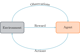
Figure 1: General reinforcement learning framework.

A recent review presented the available literature on DRL for fluid dynamics applications [30]. This work highlighted the potential of DRL in the context of fluid mechanics. To the best knowledge of the authors, at the time of writing, only two contributions proposed to exploit RL for problems related to shape optimization. These papers are concerned with the optimization of morphing airfoils with two [31] and four [32] parameters, respectively, using Q-learning methods (see section 2). In these contributions, the agent discovers the optimal morphing dynamics of airfoils in transition between different flight regimes. In addition, although not focusing on shape optimization, it is worth noting the work presented in [33], where neural networks directly learn how to perform gradient descent on specific classes of problems. The method is reported to have a very good generalization capability, which confirms it as a good candidate for shape optimization. Therefore, it appears that while DRL is a promising method for performing shape optimization, there has not been a clear illustration of direct shape optimization with DRL yet.

Therefore, motivated by our observation of the potential of DRL for performing shape optimization, we present in this article the first application of deep reinforcement learning (DRL) to direct shape optimization. We use Proximal Policy Optimization (PPO [34]) in combination with an artificial neural network to generate 2D shapes described by Bézier curves. The flow around the shape is assessed via 2D numerical simulation at moderate Reynolds numbers using FeniCs [35]. We commit to releasing all our code as open source, in order to facilitate the application of DRL to shape optimization. In the following, we first describe the methodology, including the shape generation method and the numerical setup used to compute the flow around the generated shapes. Subsequently, we introduce our reinforcement learning approach and its application to shape optimization. Finally, several results of the optimization process are presented.

2 Methodology

2.1 CFD environment

The CFD simulation, which constitutes the environment interacting with the DRL agent, consists of a computational fluid dynamics (CFD) simulation based on FeniCs [35] that numerically solves the Navier-Stokes (NS) equations. Each shape, of typical dimension 1, is immersed in a rectangular computational domain of length $l=45$ and width $w=30$ (see figure 2(a)). A constant velocity $\textbf{v}=v_{\text{in}}\textbf{e}_{x}$ is imposed on the inflow profile, while free-slip boundary conditions are imposed on top and bottom of the domain. Finally, a no-slip boundary condition is imposed on the obstacle, and a traction-free condition is set on the outflow profile. To perform the required numerical computations, mesh generation of the domain and geometries is performed using Gmsh [36]. The reference flow corresponds to that of a cylinder of radius $r_{\text{cyl}}=1$ immersed in the same domain. The reference Reynolds number is then defined as:

$$Re_{\text{ref}}=\frac{2\rho v_{\text{in}}r_{\text{cyl}}}{\mu},$$ (1)

where $\rho$ is the volumic mass of fluid, and $\mu$ its viscosity. In the remaining of this paper, $\rho$ is kept constant and equal to 1 kg/m³, as well as $v_{\text{in}}$, which is kept equal to 1 m/s. The modification of flow conditions is performed through the choice of the reference Reynolds number, which is modified by adapting the viscosity of the fluid. For all computations, the numerical timestep is chosen as:

$$\Delta t=C\,\frac{h_{\text{min}}}{v_{\text{in}}},$$ (2)

the constant $C$ being the CFL condition number (here, $C=0.5$). The drag and lift forces experienced by a given shape immersed in the flow are computed as follows:

$$f_{d}=\int_{S}\left(\bm{\sigma}\cdot\textbf{n}\right)\cdot\textbf{e}_{x}\;\text{ and }\;f_{l}=\int_{S}\left(\bm{\sigma}\cdot\textbf{n}\right)\cdot\textbf{e}_{y},$$ (3)

after what the drag and lift coefficients $C_{d}$ and $C_{l}$ are evaluated as:

$$C_{d}=\frac{f_{d}}{\frac{1}{2}\rho v_{\text{in}}^{2}s}\;\text{ and }\;C_{l}=\frac{f_{l}}{\frac{1}{2}\rho v_{\text{in}}^{2}s}.$$ (4)

In the following, a positive value of $C_{d}$ (resp $C_{l}$) indicates that the force $f_{d}$ (resp $f_{l}$) is oriented toward $\textbf{e}_{x}$ (resp $\textbf{e}_{y}$). The maximal physical time $t_{\text{max}}$ used in the numerical computations is set in order to obtain stabilized average values of the monitored quantities of interest (see next section). In practice, the following rule of thumb is used:

$$t_{\text{max}}=\frac{2}{v_{\text{in}}}\left(x_{\text{max}}-x_{\text{min}}\right).$$ (5)

The numerical formulation used for the resolution of the discretized Navier-Stokes equations is a finite-element incompressible solver based on the projection method [37], coupled to a BDF2 marching-in-time scheme. This allows us to consider flows at low Reynolds numbers, typically $Re=200$. Using this typical value of the Reynolds number allows to address a shape optimization task presenting the ingredients of non linearity and high dimensionality that are challenging in this class of problems, while keeping the computational budget limited, therefore, allowing relatively fast training without large computational resources. This is a similar approach to what was used in [28], and is well suited for a proof-of-concept of the methodology as well as future benchmarking of fine-tuned algorithms.

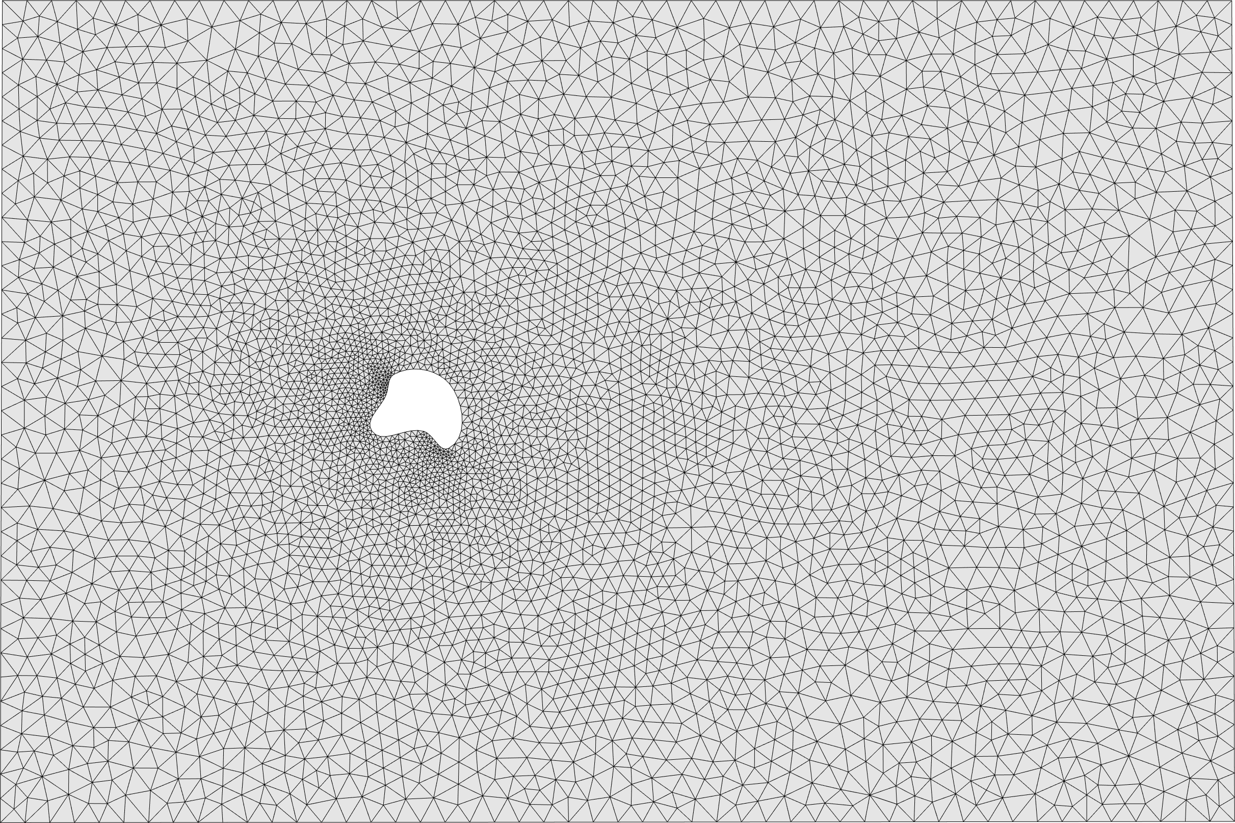
(a) Mesh of the computational domain

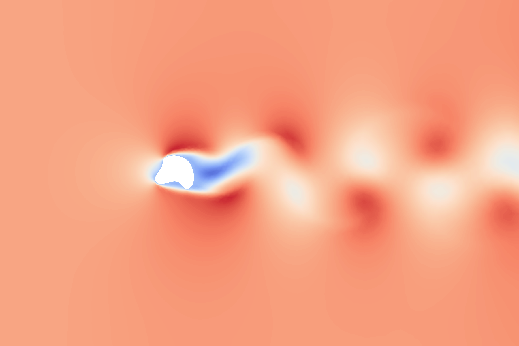
(b) Computed $v_{x}$ velocity field at $Re=200$

Figure 2: Mesh and computed $v_{x}$ velocity field at $Re=200$ behind a random shape. The recirculation area behind the obstacle is clearly visible, followed by a well-established Von Karman vortex alley. The velocity field is scaled in the $\left[-1,1\right]$ range.

2.2 Deep reinforcement learning

Our DRL agent is based on proximal policy optimization (PPO) introduced in [34]. This algorithm belongs to the class of policy gradient methods, which differs from action-value methods such as Q-learning. In action-value methods, the neural network learns to predict the future reward of taking an action when provided a given state, and selects the maximum action based on these estimates. In contrast, policy gradient methods directly optimize the expected overall reward of a decision policy mapping states to actions, without resorting to a value function. Policy gradient methods are advantageous since (i) they can handle continuous action spaces (different from Q-learning methods), and (ii) they were successfully applied to optimal control in a similar setup in the past [28].

Policy gradient methods are trained based on episodes, which correspond to a sequence of consecutive interactions of the agent with the environment. The temporally discounted sum of rewards observed during an episode acts as the quality assessment of the agent’s current decision policy. This in turn is used as the learning signal to update the network parameters via gradient descent [34]. By repeating this process, the agent iteratively learns to choose more adequate actions in order to maximize its reward (details regarding the PPO algorithm are given in appendix B).

In this work, the network action output consists of $3n$ values in $\left[-1,1\right]$, where $n$ is fixed for each experiment and corresponds to the number of points used to specify the shape. These values are then transformed adequately in order to generate a valid shape, by generating the position and local curvature of a series of points connected through a Bezier curve. Given a $(p,q,s)$ triplet provided by the network, a transformed triplet $(x,y,e)$ is obtained that generates the position $x,y$ and local curvature $e$ of the $i^{th}$ point:

$$\left\{\begin{aligned} r&=r_{\text{max}}\max\left(\left|p\right|,r_{\text{min}}\right),\\ \theta&=\frac{\pi}{n}\left(i+\frac{q}{2}\right),\\ x&=r\cos\left(\theta\right),\\ y&=r\sin\left(\theta\right),\\ e&=\frac{1}{2}\left(1+s\right).\end{aligned}\right.$$ (6)

This mapping allows to restrict the reachable positions of each point to a specific portion of a torus, bounded by user-defined interior ($r_{\text{min}}$) and exterior ($r_{\text{max}}$) radii (see figure 3). In doing so, it encourages the generation of untangled shapes, thus limiting resulting meshing issues. Once the final point positions are computed, the environment connects them to generate a closed shape using Bézier curves in a fully deterministic way (more details about the shape generation process can be found in appendix C). A CFD run is performed as described in section 2.1, and once finished, the reward is computed and passed on to the agent. The neural network representing the agent is a simple fully-connected network with two hidden layers of size 512, similar to the choice of [28]. Our training setup also benefits from parallelized multi-environment training [38], which provides an almost-linear speedup with respect to the number of available cores.

Figure 3: Example of generated shape with geometrical constraints. The colored dots indicate the control points generated by the agent, that are then joined using Bézier curves. Each point the agent suggests is restricted by construction in radius (inner and outer circles of radii $r_{\text{min}}$ and $r_{\text{max}}$) and in azimuth (diverging white lines).

2.3 Degenerate DRL

For this paper, our setup follows a ”degenerate” version of DRL where a learning episode only consists of a single timestep, i.e. a single attempt of the network to generate an optimal shape (see figure 4). Consequently, we only leverage the capability of DRL to learn from indirect supervision through a generic reward signal (note that the correct optimal response is not known, so supervised methods are not straightforwardly applicable). As will be shown in section 3, this choice allows to exploit DRL algorithms as direct non-linear optimizers. We are not aware of other works applying DRL this way.

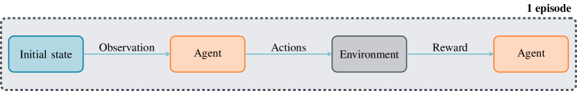
Figure 4: Degenerate reinforcement learning framework used in this paper. One episode consists of a single control from the agent: the same initial observation is provided to the agent at the start, which in return provides an action to the environment. The environment returns a reward value to the agent, and the episode is terminated.

3 Results

For the record, we are concerned with the generation of shapes maximizing the lift-to-drag ratio $\frac{C_{l}}{C_{d}}$. To this end, the proposed baseline reward is:

$$r_{t}=\left<\frac{C_{l}}{\left|C_{d}\right|}\right>-\left<\frac{C_{l}}{\left|C_{d}\right|}\right>_{\text{cyl}},$$ (7)

where the notation $<\cdot>$ indicates a temporal average over the second half of the CFD computation. The ${}_{\text{cyl}}$ subscript corresponds to the value computed in the reference case, i.e. using the unit radius cylinder. Here, the reference lift-to-drag value using the cylinder is trivially equal to 0, the cylinder generating no lift in average. The fact that this reward is sign-changing depending on the direction in which lift occurs implies a good reward variability, helping the agent to learn. Finally, shapes where no reward could be computed (meshing failed or CFD computation failed) are penalized via the reward function as follows:

$$r_{t}\leftarrow\max\left(r_{t},r_{\text{fail}}\right).$$ (8)

This shaping also allows to clip the reward in the case of shape with very bad aerodynamic properties. In practice, $r_{\text{fail}}=-5$. The deformations bounds are set as $r_{\text{min}}=0.3$ and $r_{\text{max}}=3$. The network parameters are updated every 50 shapes, with a learning rate equal to $1\text{\times}{10}^{-3}$. The shape is described with 4 points, with the possibility of keeping some of them fixed.

3.1 Baseline results

The results obtained in this configuration with 1, 3 and 4 free points out of 4 points describing the shape in total are shown in figure 5. As stated in section 2.2, one Bézier point corresponds to 3 degrees of freedom (d.o.f.) for the network to optimize (the position of the point ($x,y$) and the local curvature $e$). In the case of a single free point (figure 5(a)), the agent understands the necessity of creating a high pressure area below the shape to generate lift, and creates an airfoil-like shape with a high angle of attack. The presence of a trailing edge is also observed on all the best-performing shapes. When using three free points (figure 5(b), the same behavior is observed with a reduced apparent diameter, that is mostly controlled by the top and bottom points. The angle of attack is reduced compared to that of the single point case, while the average maximal reward is increased (see figure 7(b)). When the four points are allowed to move (figure 5(c)), the airfoil extends to the whole available domain to maximize lift, but the trailing edge remains similar (in both 3 and 4 free points cases, the angle between the center of the shape and the trailing edge is close to $23\mathrm{°}$). Although a rounded leading edge appears on the shape of figure 5(c), it did not appear systematically in the other best-performing shapes, as shown in figure 6. This is most probably due to the relatively low Reynolds number used in the present study. Finally, it should be noted that with four available points, the agent manages to obtain even better rewards, as shown in figure 7. In all cases, learning happens almost immediately, and continues almost linearly before reaching a plateau, after which the agent keeps exploring the environment, but no learning is specifically visible. The shapes shown in figures 5(a), 5(b) and 5(c) are the best ones drawn from the whole exploration. The horizontal component of the velocity field around the last shape is also shown in figure 5(d).

(a) Best shape with 4 points, 1 free point (3 d.o.f.s)

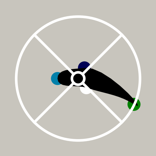
(b) Best shape with 4 points, 3 free points (9 d.o.f.s)

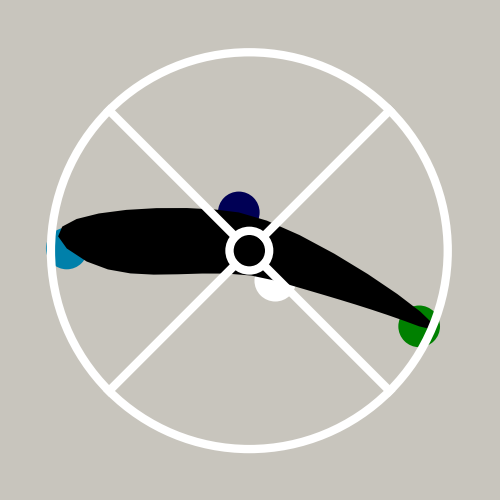
(c) Best shape with 4 points, 4 free points (12 d.o.f.s)

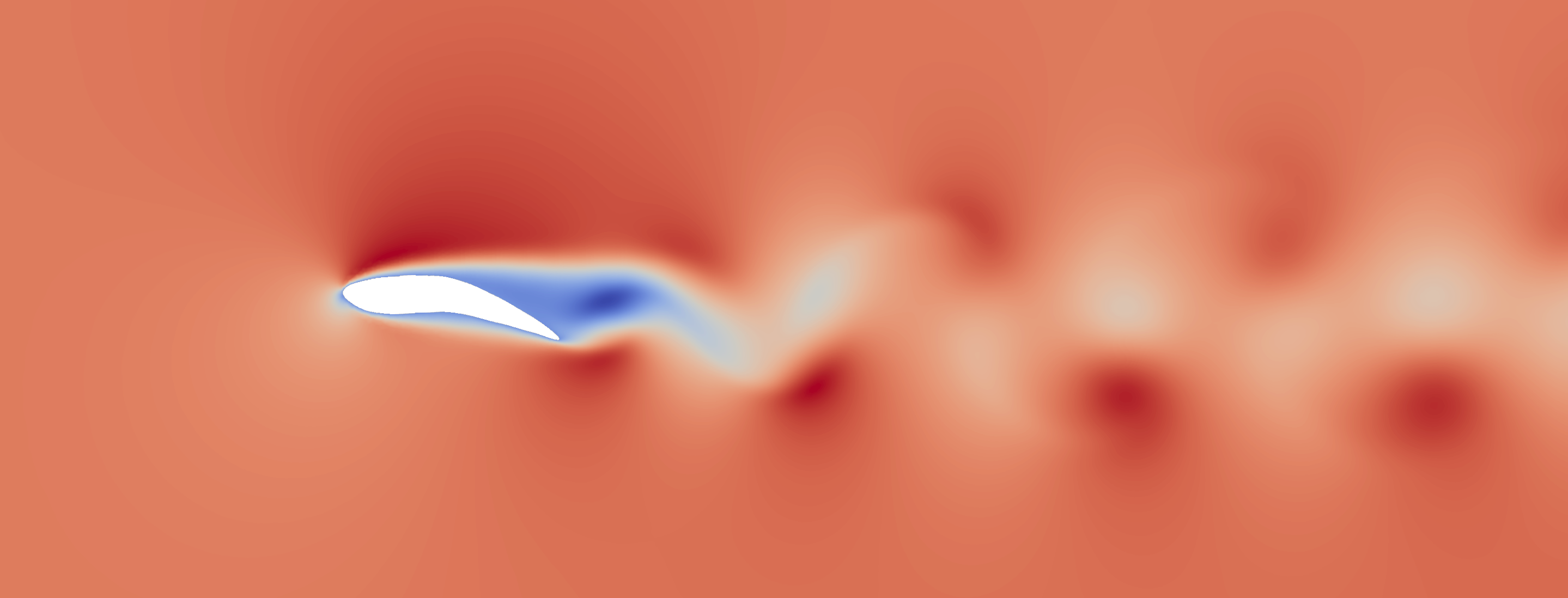
(d) Computed $v_{x}$ velocity field at $Re\sim 600$ around shape 5(c) (the domain is cropped).

Figure 5: Results of the baseline shape optimization process. Best shapes obtained using 1, 3 and 4 free points are shown in subfigures 5(a), 5(b) and 5(c) respectively. In subfigure 5(a), the left, top and bottom points are fixed to their initial position (i.e. that of the reference cylinder), while the rightmost one is free to move. In subfigure 5(b), only the left point is fixed, while in subfigure 5(c), all four points are free to move. The velocity field corresponding to shape 5(c) is shown in subfigure 5(d).

(a) Best shape with 4 free points

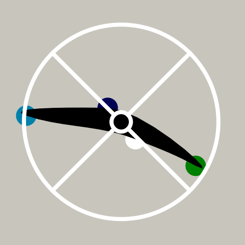
(b) Close-to-best shape with 4 free points

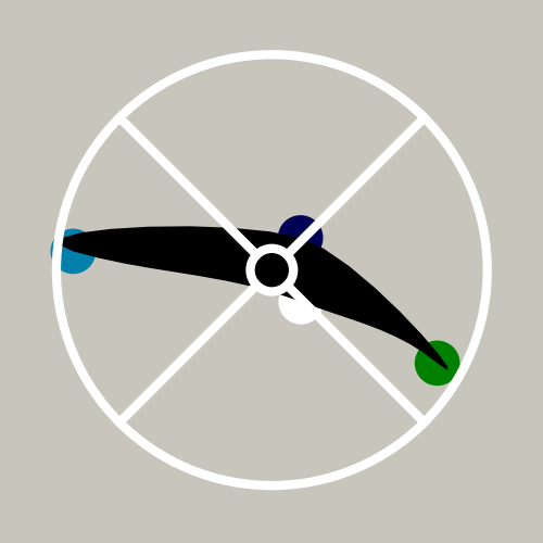
(c) Close-to-best shape with 4 free points

Figure 6: Some of the best performers using 4 free points. A rounded leading edge is not an essential feature of the best performers. This arises from the low $Re$ value used in this experiment. By contrast, the trailing edge is similar in all the best-performing shapes.

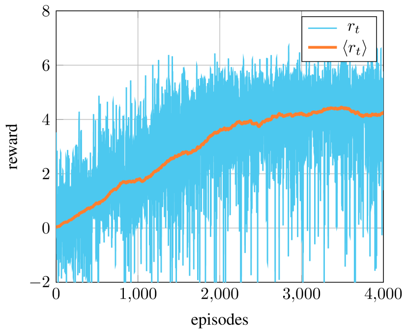
(a) Instantaneous and moving-average reward history using 4 free points

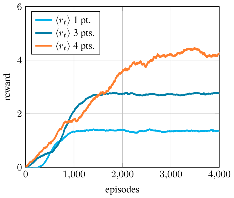
(b) Moving-average reward history using 1, 3 and 4 free points

Figure 7: Typical reward evolution (instantaneous and averaged) during the shape optimization process. Subfigure 7(a) corresponds to the learning of case 5(c). Moving-averaged learning curves for the three different cases of figure 5 are compared in subfigure 7(b).

3.2 Reward shaping

3.2.1 Shaping for faster convergence

It can be observed on figure 7(b) that the learning process requires a considerable amount of explored shapes to converge toward its final performance level. As could be expected, this number of shapes increases with the number of degrees of freedom involved in the shape generation. In this section, we show that basic reward shaping is enough, in our case, to cut that number by a considerable amount. To do so, the reward is computed following equations (7) and (8), after which it is multiplied by a constant if it is positive, as shown in figure 8(a), following:

$$r_{t}\leftarrow 2\,r_{t}\cdot\mathds{1}\big{(}r_{t}>0\big{)}.$$ (9)

The impact of this modification on the learning is clearly visible in figure 8(b): when using the shaped reward, the agent reaches the learning plateau after approximatively 1500 shapes, versus 3000 when using the baseline reward. The average plateau reward is also slightly higher with the shaped reward.

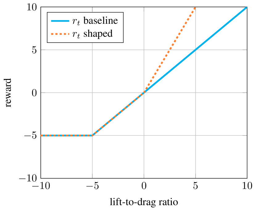
(a) Baseline and shaped reward functions as a function of lift-to-drag ratio

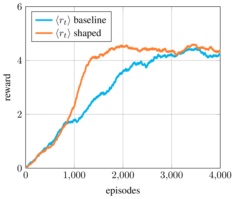
(b) Average reward observed during agent learning using baseline and shaped reward functions (normalized)

Figure 8: Baseline and shaped reward functions and their resulting observed rewards on the 4 free points case. Using a shaped reward increases the overall learning speed.

3.2.2 Shaping to add constraints

Constraints can be weakly enforced (in a non-mathematical sense) by adding penalties to the reward function that eventually prohibits undesired behaviors from the network. By regularly hitting a reward barrier in the action space, the agent will learn to avoid the associated behavior. Here, the goal is to prescribe the area of the optimal shape to remain close to that of the initial cylinder. To that end, one can simply add an ad hoc penalization term to the reward function:

$$r_{t}\leftarrow r_{t}-\frac{\left|\alpha-\alpha_{\text{cyl}}\right|}{\alpha_{\text{cyl}}},$$ (10)

where $\alpha$ is the area of the current shape, and $\alpha_{\text{cyl}}$ is the area of the reference cylinder. In figure 9, we compare the optimal shapes obtained using 4 points with 3 moving points, both with and without the area penalization (10). The area of the optimal shape with penalization is very close to that of the reference cylinder, which is not the case of the baseline one. As shown in figure 10, during the first 2000 episodes, both the constrained and unconstrained agents produce shapes of similar areas. Once the learning plateau is reached, the constrained agent starts generating shapes that minimize the penalization term in (10). Although this effect is barely visible on the reward curves, the behavior is particularly clear when looking at the area history. The lower $\left<r_{t}\right>$ values for the constrained agent are a direct consequence of the trade-off between the lift-to-drag ratio and the area penalization. This additional constraint induces a reduction of approximately 30% in the lift-to-drag ratio compared to the optimal shape without area penalization.

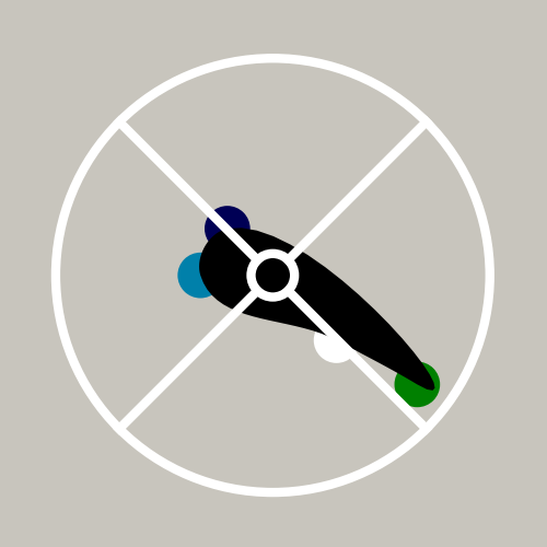
(a) Best shape with 4 points, 3 free points, with area penalization ($\alpha=3.176$)

(b) Best shape with 4 points, 3 free points, no area penalization ($\alpha=2.733$)

Figure 9: Optimal shapes obtained with and without area penalization using 4 points with 3 free points. While the target area is that of the unit cylinder ($\alpha_{\text{cyl}}=\pi$), the area of the optimal shape with area penalization is equal to 3.176, versus 2.733 for that of the non-penalized shape. While respecting this constraint, the lift-to-drag ratio of the penalized shape is approximately 30% lower than that of the non-penalized one.

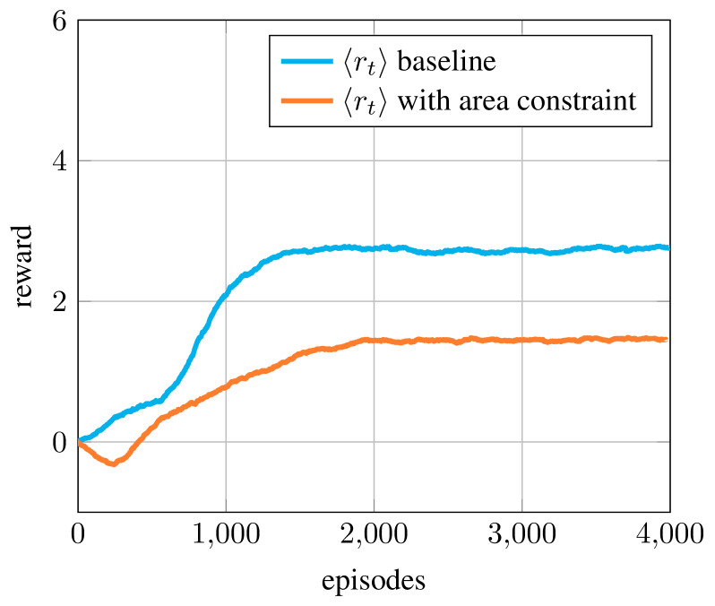
(a) Moving-average reward history with and without area constraint

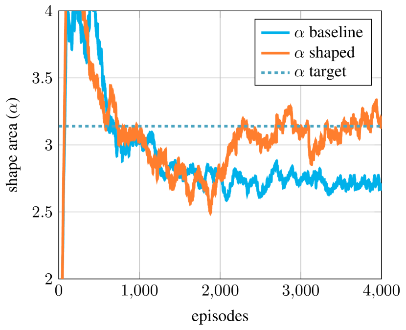
(b) Moving-average area history with and without area constraint

Figure 10: Moving-average reward and area history of the explored shapes using baseline and shaped reward (10) compared to target area on a single training. Once the learning plateau is reached (approx. 2000 episodes), the agent modifies its behavior in order to fulfill the additional area constraint, although this is barely visible on the reward curve. For the case with area constraint, the agent has to make a trade-off between the lift-to-drag ratio and the area penalization in the reward, explaining the lower $\left<r_{t}\right>$ values.

4 Conclusions

In this work, we present the first application of deep reinforcement learning to direct shape optimization. After an introduction to the basic concepts of DRL and a description of the CFD setup, details were given on the shape generation using Bézier curves and the implementation of the DRL environment. Then, we showed that, provided an adequate reward function based on the lift-to-drag ratio, our agent generated wing-like optimal shapes without any priori knowledge of aerodynamic concepts. Furthermore, we explored reward shaping, both to speed up learning and to introduce additional constraint on the considered optimization problem. This paper also introduced a ”degenerate DRL” approach that allows to use DRL algorithms as general purpose optimizers. Many refinements of the method remain to be explored, regarding the observations provided to the agent, the management of the shape deformation, or the data efficiency of the method, among others.

This contribution paves way to a new category of shape optimization processes. Although our application is focused on aerodynamics, the method is agnostic to the application use case, which makes our approach easily extendable to other domains of computational mechanics. In addition, using DRL for performing shape optimization may offer several promising perspectives. First, the DRL methodology can be expected to handle non-linear, high dimensionality optimization problems well, as this has already been proven in a number of control applications. Second, DRL is known to scale well to large amounts of data, which is well adapted to cases where parallelization of simulations is difficult due to algorithmic or hardware challenges, but many simulations can be run in parallel. Third, we can expect that transfer learning may enable DRL to solve similar new problems solely based on the knowledge obtained from its previous training. Further work should be performed to investigate each of these aspects.

Appendix A Open source code

The code of this project is available on the following Github repository: https://github.com/jviquerat/drl_shape_optimization. It relies on FEniCS for the CFD resolution [35], and on Tensorforce [39] for the reinforcement learning library. The generation of shapes using Bézier curves description is ensured by a homemade code included in the repository.

Appendix B DRL, policy gradient and PPO algorithm

This section briefly introduces the basic concepts and definitions of DRL, policy gradient and proximal policy optimization methods. For a more detailed introduction and discussion, the reader is referred to [40] and references therein for more details.

Reinforcement learning is a class of machine learning methods focusing on optimal decision making in a complex environment. At any discrete timestep $t\in\mathbb{N}$, an agent observes the current world state $s_{t}$, decides for an action $a_{t}$ and receives a reward signal $r_{t}\in\mathbb{R}$. In the literature, observation and state are sometimes distinguished, but for ease of notation, these two concepts are commonly merged into the concept of a state $s_{t}$ (which we do here). Still, the reader must keep in mind that states are often a partial and/or noisy observation of the actual state of the environment. The final goal of the agent is to update the discounted cumulative reward over a rollout of the agent’s policy $\pi$, i.e. a trajectory of states, actions and rewards $\tau=(s_{0},a_{0},r_{0}s_{1},a_{1},r_{1},...)$ which distribution follows policy $\pi$:

$$R(\tau)=\sum_{t=0}^{T}\gamma^{t}r_{t},$$

where $\gamma\in\left[0,1\right]$ is a discount factor to prioritize more immediate over more distant rewards. Two popular types of reinforcement learning algorithms are Q-learning and policy gradient methods:

1. Q-learning assumes a discrete, finite action space, and chooses actions based on their estimated Q-value, which is the expected discounted cumulative reward obtained when starting from state $s$ with action $a$, and then following trajectory $\tau$ according to policy $\pi$:

   $$Q(s,a)=\underset{\tau\sim\pi}{\mathbb{E}}\left[R(\tau)|s,a\right].$$

   In DRL, the $Q$ function is implemented as a deep neural network and optimized to fit the recursively characterized optimal solution, given by the Bellman equation:

   $$Q^{*}(s,a)=R(s,a)+\gamma\max_{a^{\prime}}Q^{*}(s^{\prime},a^{\prime}).$$

2. Policy gradient (PG) methods, on the other hand, can handle both discrete and continuous action spaces. In contrast to Q-learning, PG methods directly optimize the policy instead of an auxiliary value function. They assume a stochastic policy $\pi(a|s)$, often parameterized by a deep neural network, whose gradient-based optimization directly maximizes the expected discounted cumulative reward $\underset{\tau\sim\pi}{\mathbb{E}}\left[R\right]$, approximated by a finite batch of rollouts. Compared to Q-learning methods, PG methods exhibit better capabilities in handling high dimensional action spaces as well as smoother convergence properties, although they are known to often converge to local minima.

Introduced in 2000 by Sutton et al [41], vanilla PG relies on an estimate of the first-order gradient of the log-policy $\nabla_{\theta}\log\pi_{\theta}$ to update its network. This approach was latter followed by several major improvements, including the trust-region policy optimization (TRPO) [42] and the proximal policy optimization (PPO) [34]. In these methods, the network update exploits a surrogate advantage functional:

$$\theta_{k+1}=\arg\max_{\theta}L(\theta_{k},\theta),$$

with

$$L(\theta_{k},\theta)=\underset{(s,a)\sim\pi_{\theta_{k}}}{\mathbb{E}}\big{[}\Pi(s,a,\theta,\theta_{k})A^{\pi_{\theta_{k}}}(s,a)\big{]},$$

and

$$\Pi(s,a,\theta,\theta_{k})=\frac{\pi_{\theta}(a|s)}{\pi_{\theta_{k}}(a|s)}.$$

In the latter expressions, $A^{\pi_{\theta_{k}}}(s,a)$ is called the advantage function, and measures how much better it is to take action $a$ in state $s$ compared to the average result of all actions that could be taken in state $s$. Hence, $L(\theta_{k},\theta)$ measures how much better (or worse) policy $\pi_{\theta}$ performs compared to the previous policy $\pi_{\theta_{k}}$. In order to avoid too large policy updates that could collapse the policy performance, TRPO leverages second-order natural gradient optimization to update parameters within a trust-region of a fixed maximum Kullback-Leibler divergence between old and updated policy distribution. This relatively complex approach was replaced in the PPO method by simply clipping the maximized expression:

$$L(\theta_{k},\theta)=\underset{(s,a)\sim\pi_{\theta_{k}}}{\mathbb{E}}\big{[}\min\left(\Pi(s,a,\theta,\theta_{k})A^{\pi_{\theta_{k}}}(s,a),g\left(\varepsilon,A^{\pi_{\theta_{k}}}(s,a)\right)\right)\big{]},$$

where

$$g(\varepsilon,A)=\begin{cases}(1+\varepsilon)A&A\geq 0,\\ (1-\varepsilon)A&A<0,\end{cases}$$

where $\varepsilon$ is a small, user-defined parameter. When $A^{\pi_{\theta_{k}}}(s,a)$ is positive, taking action $a$ in state $s$ is preferable to the average of all actions that could be taken in that state, and it is natural to update the policy to favor this action. Still, if the ratio $\Pi(s,a,\theta,\theta_{k})$ is very large, stepping too far from the previous policy $\pi_{\theta_{k}}$ could damage performance. For that reason, $\Pi(s,a,\theta,\theta_{k})$ is clipped to $1+\varepsilon$ to avoid too large updates of the policy. If $A^{\pi_{\theta_{k}}}(s,a)$ is negative, taking action $a$ in state $s$ represents a poorer choice than the average of all actions that could be taken in that state, and it is natural to update the policy to decrease the probability of taking this action. In the same fashion, $\Pi(s,a,\theta,\theta_{k})$ is clipped to $1-\varepsilon$ if it happens to be lower than that value.

In the latter expressions, $A^{\pi_{\theta_{k}}}(s,a)$ is estimated using a generalized advantage estimator (GAE), which represents a trade-off between Monte-Carlo and time difference estimators [43]. Additionally, instead of performing a single, full-batch update, the network optimization is decomposed in multiple updates computed from subsampled mini-batches. Finally, an entropy regularization is added to the surrogate loss:

$$L(\theta_{k},\theta)=\underset{(s,a)\sim\pi_{\theta_{k}}}{\mathbb{E}}\big{[}\min\left(\Pi(s,a,\theta,\theta_{k})A^{\pi_{\theta_{k}}}(s,a),g\left(\varepsilon,A^{\pi_{\theta_{k}}}(s,a)\right)\right)\big{]}+cH\left(\pi_{\theta}(a|s)\right).$$

This additional term encourages the agent not to be over-confident, by keeping the policy distribution close to uniform unless there is a strong signal not to.

Appendix C Shape generation using Bézier curves

This section describes the process followed to generate shapes from a set of $n_{s}$ points provided by the agent. Once the points are collected, an ascending trigonometric angle sort is performed (see figure 11(a)), and the angles between consecutive points are computed. An average angle is then computed around each point (see figure 11(b)) using:

$$\theta^{*}_{i}=\alpha\theta_{i-1,i}+(1-\alpha)\theta_{i,i+1},$$

with $\alpha\in\left[0,1\right]$. The averaging parameter $\alpha$ allows to alter the sharpness of the curve locally, maximum smoothness being obtained for $\alpha=0.5$. Then, each pair of points is joined using a cubic Bézier curve, defined by four points: the first and last points, $p_{i}$ and $p_{i+1}$, are part of the curve, while the second and third ones, $p^{*}_{i}$ and $p^{**}_{i}$, are control points that define the tangent of the curve at $p_{i}$ and $p_{i+1}$. The tangents at $p_{i}$ and $p_{i+1}$ are respectively controlled by $\theta^{*}_{i}$ and $\theta^{*}_{i+1}$ (see figure 11(c)). A final sampling of the successive Bézier curves leads to a boundary description of the shape (figure 11(d)). Using this method, a wide variety of shapes can be attained.

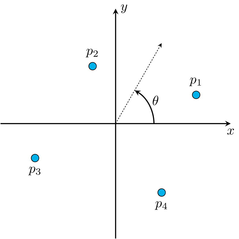
(a) Sort the provided points by ascending trigonometric angle

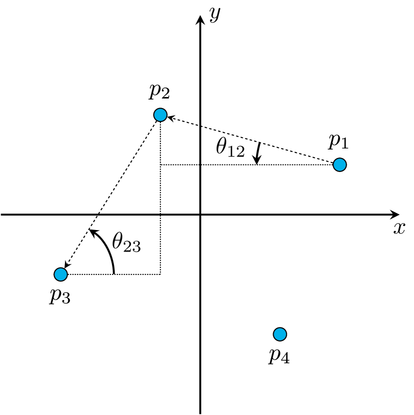
(b) Compute angles between points, and compute an average angle around each point $\theta^{*}_{i}$

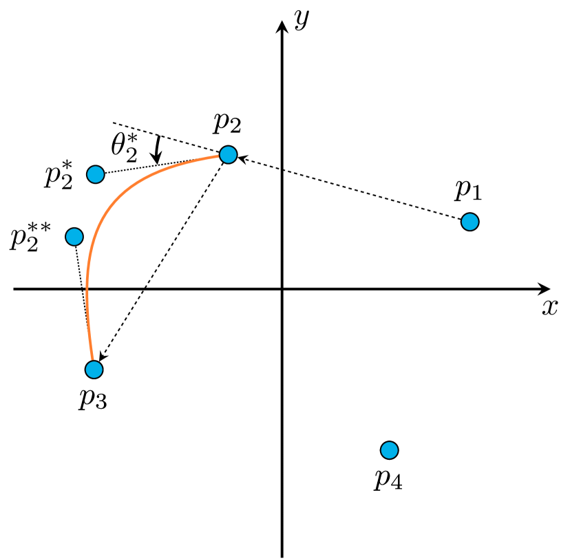
(c) Compute control points coordinates from averaged angles and generate cubic Bézier curve

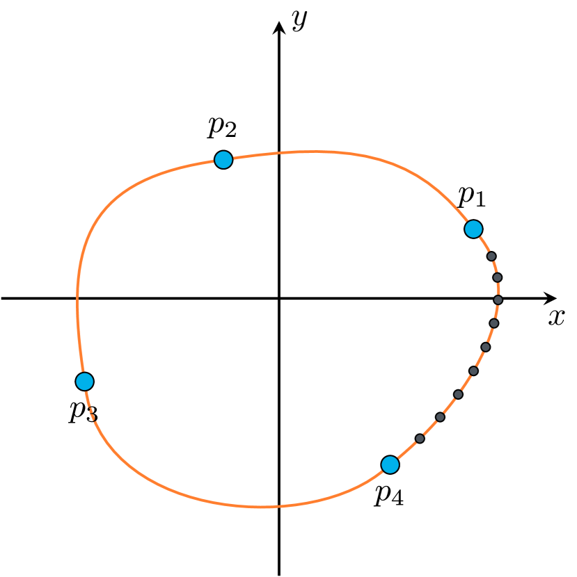
(d) Sample all Bézier lines and export for mesh immersion

Figure 11: Shape generation using cubic Bézier curves. Each subfigure illustrates one of the consecutive steps used in the process. Detailed nomenclature is provided in the text.

References

- [1] Grégoire Allaire, Eric Bonnetier, Gilles Francfort, and François Jouve. Shape optimization by the homogenization method. Numerische Mathematik, 76(1):27–68, 1997.
- [2] Johannes Semmler, Lukas Pflug, Michael Stingl, and Günter Leugering. Shape Optimization in Electromagnetic Applications. Springer International Publishing, 2015.
- [3] Wolf Hucho and Gino Sovran. Aerodynamics of road vehicles. Annual review of fluid mechanics, 25(1):485–537, 1993.
- [4] Antony Jameson. Aerodynamic shape optimization using the Adjoint Method. VKI Lecture Series, 30, 2003.
- [5] Byungwook Jang, Myungjun Kim, Jungsun Park, and Sooyong Lee. Design optimization of composite radar absorbing structures to improve stealth performance. International Journal of Aeronautical and Space Sciences, 17(1):20–28, 2016.
- [6] Alison L Marsden, Meng Wang, Bijan Mohammadi, and P Moin. Shape optimization for aerodynamic noise control. Center for Turbulence Research Annual Brief, pages 241–247, 2001.
- [7] H. W. Carlson and W. D. Middleton. A numerical method for the design of camber surfaces of supersonic wings with arbitrary planforms. NASA Technical Reports, 1964.
- [8] J. Reuther, A. Jameson, J. Farmer, L. Martinelli, and D. Saunders. Aerodynamic shape optimization of complex aircraft configurations via an adjoint formulation. In American Institute of Aeronautics and Astronautics, editor, Proc. AIAA Aerospace Sciences Meeting and Exhibit, 2013.
- [9] Thomas A. Zang. Airfoil/Wing Optimization. Encyclopedia of Aerospace Engineering, pages 1–11, 2010.
- [10] Gaetan K. W. Kenway and Joaquim R. R. A. Martins. Multipoint Aerodynamic Shape Optimization Investigations of the Common Research Model Wing. AIAA Journal, 54(1):113–128, 2015.
- [11] O. Pironneau. On optimum design in fluid mechanics. Journal of Fluid Mechanics, 64:97 – 110, 1974.
- [12] S. N. Skinner and H. Zare-Behtash. State-of-the-art in aerodynamic shape optimisation methods. Applied Soft Computing Journal, 62:933–962, 2018.
- [13] W. Yamazaki, K. Matsushima, and K. Nakahashi. Aerodynamic design optimization using the drag-decomposition method. AIAA Journal, 46(5):1096–1106, 2008.
- [14] Yuan-yuan Wang, Bin-qian Zhang, and Ying-chun Chen. Robust airfoil optimization based on improved particle swarm optimization method. Applied Mathematics and Mechanics, 32(10):1245, 2011.
- [15] Rania Hassan, Babak Cohanim, Olivier de Weck, and Gerhard Venter. A comparison of particle swarm optimization and the genetic algorithm. In American Institute of Aeronautics and Astronautics, editor, 46th AIAA/ASME/ASCE/AHS/ASC Structures, Structural Dynamics and Materials Conference, 2012.
- [16] W. T. Tiow, K. F C. Yiu, and M Zangeneh. Application of simulated annealing to inverse design of transonic turbomachinery cascades. Proceedings of the Institution of Mechanical Engineers, Part A: Journal of Power and Energy, 216(1):59–73, 2002.
- [17] Slawomir Koziel, Yonatan Tesfahunegn, Anand Amrit, and Leifur T. Leifsson. Rapid multi-objective aerodynamic design using co-kriging and space mapping. In American Institute of Aeronautics and Astronautics, editor, 57th AIAA/ASCE/AHS/ASC Structures, Structural Dynamics, and Materials Conference, 2016.
- [18] Nestor V. Queipo, Raphael T. Haftka, Wei Shyy, Tushar Goel, Rajkumar Vaidyanathan, and P. Kevin Tucker. Surrogate-based analysis and optimization. Progress in Aerospace Sciences, 41(1):1–28, 2005.
- [19] Oleg Chernukhin and David W. Zingg. Multimodality and global optimization in aerodynamic design. AIAA Journal, 51(6):1342–1354, 2013.
- [20] Sergey Peigin and Boris Epstein. Multiconstrained aerodynamic design of business jet by cfd driven optimization tool. Aerospace Science and Technology, 12(2):125 – 134, 2008.
- [21] Pierluigi Della Vecchia and Fabrizio Nicolosi. Aerodynamic guidelines in the design and optimization of new regional turboprop aircraft. Aerospace Science and Technology, 38:88 – 104, 2014.
- [22] Aaron Courville Ian Goodfellow, Yoshua Bengio. The Deep Learning Book. MIT Press, 2017.
- [23] Steven L. Brunton, Bernd R. Noack, and Petros Koumoutsakos. Machine learning for fluid mechanics. Annual Review of Fluid Mechanics, 52(1):477–508, 2020.
- [24] Volodymyr Mnih, David Silver, and Martin Riedmiller. Atari Deep Reinforcement learning. Nips, pages 1–9, 2013.
- [25] David Silver, Julian Schrittwieser, Karen Simonyan, Ioannis Antonoglou, Aja Huang, Arthur Guez, Thomas Hubert, Lucas Baker, Matthew Lai, Adrian Bolton, et al. Mastering the game of go without human knowledge. Nature, 550(7676):354, 2017.
- [26] Noam Brown and Tuomas Sandholm. Superhuman ai for multiplayer poker. Science, 2019.
- [27] Nicolas Heess, Dhruva TB, Srinivasan Sriram, Jay Lemmon, Josh Merel, Greg Wayne, Yuval Tassa, Tom Erez, Ziyu Wang, S. M. Ali Eslami, Martin Riedmiller, and David Silver. Emergence of Locomotion Behaviours in Rich Environments. arXiv e-prints, 2017.
- [28] Jean Rabault, Miroslav Kuchta, Atle Jensen, Ulysse Reglade, and Nicolas Cerardi. Artificial Neural Networks trained through Deep Reinforcement Learning discover control strategies for active flow control. Journal of Fluid Mechanics, 865:281–302, 2019.
- [29] Hongzi Mao, Mohammad Alizadeh, Ishai Menache, and Srikanth Kandula. Resource Management with Deep Reinforcement Learning. arXiv e-prints, pages 50–56, 2016.
- [30] Paul Garnier, Jonathan Viquerat, Jean Rabault, Aurélien Larcher, Alexander Kuhnle, and Elie Hachem. A review on deep reinforcement learning for fluid mechanics. arXiv e-prints, 2019.
- [31] Amanda Lampton, Adam Niksch, and John Valasek. Reinforcement learning of a morphing airfoil-policy and discrete learning analysis. Journal of Aerospace Computing, Information, and Communication, 7(8):241–260, 2010.
- [32] Amanda Lampton, Adam Niksch, and John Valasek. Morphing Airfoils with Four Morphing Parameters. In American Institute of Aeronautics and Astronautics, editor, AIAA Guidance, Navigation and Control Conference and Exhibit, 2008.
- [33] Marcin Andrychowicz, Misha Denil, Sergio Gomez, Matthew W. Hoffman, David Pfau, Tom Schaul, Brendan Shillingford, and Nando de Freitas. Learning to learn by gradient descent by gradient descent. arXiv e-prints, pages 1–17, 2016.
- [34] John Schulman, Filip Wolski, Prafulla Dhariwal, Alec Radford, and Oleg Klimov. Proximal Policy Optimization Algorithms. arXiv e-prints, pages 1–12, 2017.
- [35] Martin S. Alnæs, Jan Blechta, Johan Hake, August Johansson, Benjamin Kehlet, Anders Logg, Chris Richardson, Johannes Ring, Marie E. Rognes, and Garth N. Wells. The fenics project version 1.5. Archive of Numerical Software, 3(100), 2015.
- [36] Christophe Geuzaine and Jean-François Remacle. A three-dimensional finite element mesh generator with built-in pre- and post-processing facilities. Int. J. Numer. Meth. Engng., 79(11):1309–1331, 2017.
- [37] J. L. Guermond, P. Minev, and Jie Shen. An overview of projection methods for incompressible flows. Computer Methods in Applied Mechanics and Engineering, 195(44-47):6011–6045, 2006.
- [38] Jean Rabault and Alexander Kuhnle. Accelerating deep reinforcement learning of active flow control strategies through a multi-environment approach. Physics of Fluids, 31:094105, 2019.
- [39] Alexander Kuhnle, Michael Schaarschmidt, and Kai Fricke. Tensorforce: a tensorflow library for applied reinforcement learning. Web page, 2017.
- [40] Vincent François-lavet, Peter Henderson, Riashat Islam, and Marc G Bellemare. An Introduction to Deep Reinforcement Learning. Foundations and trends in machine learning, 2018.
- [41] Richard S Sutton, David McAllester, Satinder Singh, and Yishay Mansour. Policy Gradient Methods for Reinforcement Learning with Function Approximation Richard. Advances in Neural Information Processing Systems, 12:1057–1063, 2000.
- [42] John Schulman, Sergey Levine, Philipp Moritz, Michael I. Jordan, and Pieter Abbeel. Trust Region Policy Optimization. arXiv e-prints, 2015.
- [43] John Schulman, Philipp Moritz, Sergey Levine, Michael Jordan, and Pieter Abbeel. High-Dimensional Continuous Control Using Generalized Advantage Estimation. arXiv e-prints, pages 1–14, 2015.