A Weakly Supervised Method for Instance Segmentation of Biological Cells

Abstract

We present a weakly supervised deep learning method to perform instance segmentation of cells present in microscopy images. Annotation of biomedical images in the lab can be scarce, incomplete, and inaccurate. This is of concern when supervised learning is used for image analysis as the discriminative power of a learning model might be compromised in these situations. To overcome the curse of poor labeling, our method focuses on three aspects to improve learning: i) we propose a loss function operating in three classes to facilitate separating adjacent cells and to drive the optimizer to properly classify underrepresented regions; ii) a contour-aware weight map model is introduced to strengthen contour detection while improving the network generalization capacity; and iii) we augment data by carefully modulating local intensities on edges shared by adjoining regions and to account for possibly weak signals on these edges. Generated probability maps are segmented using different methods, with the watershed based one generally offering the best solutions, specially in those regions where the prevalence of a single class is not clear. The combination of these contributions allows segmenting individual cells on challenging images. We demonstrate our methods in sparse and crowded cell images, showing improvements in the learning process for a fixed network architecture.

1 Introduction

In developmental cell biology studies, one generally needs to quantify temporal signals, e.g. protein concentration, on a per cell basis. This requires segmenting individual cells in many images, accounting to hundreds or thousands of cells per experiment. Such data availability suggests carrying on large annotation efforts, following the common wisdom that massive annotations are beneficial for fully supervised training to avoid overfitting and improve generalization. However, full annotation is expensive, time consuming, and it is often inaccurate and incomplete when it is done at the lab, even by specialists (see Fig.1).

Figure 1: Incomplete (A) and inaccurate (B) annotations of training images might be harmful for supervised learning as the presence of similar regions with erratic annotations might puzzle the optimization process. Our formulation is able to segment well under uncertainty as shown in the examples in the right panels of A and B above.

 

To mitigate these difficulties and make the most of limited training data, we work on three fronts to improve learning. In addition to the usual data augmentation strategies (rotation, cropping, etc.), we propose a new augmentation scheme which modulates intensities on the borders of adjacent cells as these are key regions when separating crowded cells. This scheme augments the contrast patterns between edges and cell interiors. We also explicitly endow the loss function to account for critically underrepresented and reduced size regions so they can have a fair contribution to the functional during optimization. By adopting large weights on short edges separating adjacent cells we increase the chances of detecting them as they now contribute more significantly to the loss. In our experience, without this construction, these regions are poorly classified by the optimizer – weights used in the original U-Net formulation [9] are not sufficient to promote separation of adjoining regions. Further, adopting a three classes approach [4] has significantly improved the separation of adjacent cells which are otherwise consistently merged when considering a binary foreground and background classification strategy. We have noticed that complex shapes, e.g. with small necks, slim invaginations and protrusions, are more difficult to segment when compared to round, mostly convex shapes [10]. Small cells, tiny edges, and slim parts, equally important for the segmentation result, can be easily dismissed by the optimizer if their contribution is not explicitly accounted for and on par with other more dominant regions.

Previous Work. In [6] the authors propose a weakly semantic segmentation method for biomedical images. They include prior knowledge in the form of constraints into the loss function for regularizing the size of segmented objects. The work in [11] proposes a way to keep annotations at a minimum while still capturing the essence of the signal present in the images. The goal is to avoid excessively annotating redundant parts, present due to many repetitions of almost identical cells in the same image. In [8] the authors also craft a tuned loss function applied to improve segmentation on weakly annotated gastric cancer images. The instance segmentation method for natural images Mask R-CNN [5] uses two stacked networks, with detection followed by segmentation. We use it for comparisons on our cell images. Others have used three stacked networks for semantic segmentation and regression of a watershed energy map allowing separating nearby objects [1].

2 Segmentation Method

Notation. Let $S=\{(x_{j},g_{j})\}_{j=1}^{N}$ be a training instance segmentation set where $x_{j}\colon\Omega\to\mbox{$\mathbbm{R}$}^{+}$ is a single channel gray image defined on the regular grid $\Omega\in\mbox{$\mathbbm{R}^{2}$}$, and $g_{j}\colon\Omega\to\{0,\ldots,m_{j}\}$ its instance segmentation ground truth map which assigns to a pixel $p\in\Omega$ a unique label $g_{j}(p)$ among all $m_{j}+1$ distinct instance labels, one for each object, including background, labeled 0. For a generic $(x,g)$, $V_{i}=\{p\;|\;g(p)=i\}$ contains all pixels belonging to instance object $i$, hence forming the connected component of object $i$. Due to label uniqueness, $V_{i}\cap V_{j}=\O,i\neq j$, i.e. a pixel cannot belong to more than one instance thus satisfying the panoptic segmentation criterion [7]. Let $h\colon\Omega\to\{0,\ldots,C\}$ be a semantic segmentation map, obtained using $g$, which reports the semantic class of a pixel among the $C+1$ possible semantic classes, and $y\colon\Omega\to\mbox{$\mathbbm{R}^{C+1}$}$ its one hot encoding mapping. That is, for vector $y(p)\in\mbox{$\mathbbm{R}^{C+1}$}$ and its $l$-th component $y_{l}(p)$, we have $y_{l}(p)=1$ iff $h(p)=l$, otherwise $y_{l}(p)=0$. We call $n_{l}=\sum_{p\in\Omega}y_{l}(p)$ the number of pixels of class $l$, and $\eta_{k}(p),k\geqslant 1$, the $(2k+1)\times(2k+1)$ neighborhood of a pixel $p\in\Omega$. In our experiments we adopted $k=2$.

From Instance to Semantic Ground Truth. We formulate the instance segmentation problem as a semantic segmentation problem where we obtain object segmentation and separation of cells at once. To transform an instance ground truth to a semantic ground truth, we adopted the three semantic classes scheme of [4]: image background, cell interior, and touching region between cells. This is suitable as the intensity distribution of our images in those regions is multi-modal. We define our semantic ground truth $h$ as

$$h(p)=\left\{\begin{aligned} 0&\quad\text{ if }g(p)=0&\text{-- background}\\ 2&\quad\text{ if }\sum\nolimits_{p^{\prime}\in\eta_{k}(p)}[g(p^{\prime})\neq g(p)]\cdot[g(p^{\prime})\neq 0]>1&\text{-- touching}\\ 1&\quad\text{ otherwise}&\text{-- cell}\end{aligned}\right.\vspace{-1mm}$$ (1)

where $[\cdot]$ refers to Iverson bracket notation [2]: $[b]=1$ if the boolean condition $b$ is true, otherwise $[b]=0$. Eq.1 assigns class $0$ to all background pixels, it assigns class $2$ to all pixels whose neighborhood $\eta_{k}$ contains at least one pixel of another connected component, and it assigns class $1$ to cell pixels not belonging to touching regions.

\begin{overpic}[width=84.55907pt]{images/fig1a_-10.png} \put(65.0,85.0){\color[rgb]{1,1,1}$\displaystyle-1.0$} \end{overpic}

\begin{overpic}[width=84.55907pt]{images/fig1b_-05.png} \put(65.0,85.0){\color[rgb]{1,1,1}$\displaystyle-0.5$} \end{overpic}

\begin{overpic}[width=84.55907pt]{images/fig1c_0.png} \put(70.0,85.0){\color[rgb]{1,1,1}$\displaystyle 0.0$} \end{overpic}

\begin{overpic}[width=84.55907pt]{images/fig1d_05.png} \put(70.0,85.0){\color[rgb]{1,1,1}$\displaystyle 0.5$} \end{overpic}

\begin{overpic}[width=84.55907pt]{images/fig1e_10.png} \put(70.0,85.0){\color[rgb]{1,1,1}$\displaystyle 1.0$} \end{overpic}

Figure 2: Contrast modulation around touching regions. Separating adjacent cells is one of the major challenges in crowded images. To leverage learning, we feed the network with a variety of contrasts around touching regions. We do so by modulating their intesities while keeping adjacencies the same. In this example, an original image ($a=0$) has its contrast increased (decreased) around shared edges when we set $a<0$ ($a>0$).

 

Touching Region Augmentation. Touching regions have the lowest pixel count among all semantic classes, having few examples to train the network. They are in general brighter than their surroundings, but not always, with varying values along its length. To train with a larger gamut of touching patterns, including weak edges, we augment existing ones by modulating their pixel values according to the expression $x_{a}(p)=(1-a)\cdot x(p)+a\cdot\tilde{x}(p)$, only applied when $h(p)=2$, where $\tilde{x}$ is the $7\times 7$ median filtered image of $x$. When $a<0\;(a>0)$ we increase (decrease) contrast. During training, we have random values of $a\sim U(-1,1)$. An example of this modulation is shown in Fig.2.

Loss Function. U-Net [9] is an encoder–decoder network for biomedical image segmentation with proven results in small datasets, and with cross entropy being the most commonly adopted loss function. The weighted cross entropy [9] is a generalization where a pre–computed weight map assigns to each pixel its importance for the learning process,

$$\mathcal{L}(y,z)=-\sum_{l=0}^{C}\sum_{p\in\Omega}\omega_{\beta,\nu,\sigma}(p)\cdot y_{l}(p)\cdot\log z_{l}(p)\vspace{-1mm}$$ (2)

where $\omega_{\beta,\nu,\sigma}(p)$ is the parameterized weight at pixel $p$, and $z_{l}(p)$ the computed probability of $p$ belonging to class $l$ for ground truth $y_{l}(p)$.

Let $R(u)=u^{+}$ be the rectified linear function, ReLu, and $\varphi_{\beta}(u)=R(1-u/\beta),u\in\mbox{$\mathbbm{R}$}$, a rectified inverse function saturated in $\beta\in\mbox{$\mathbbm{R}$}^{+}$. We propose the Triplex Weight Map, $W^{3}$, model

$$\omega_{\beta,\nu,\sigma}(p)=\begin{cases}\nu/n_{0}+\nu\cdot\varphi_{\beta}\left(\phi_{h}(p)\right)/n_{1}&\text{ if }h(p)=0\\ \nu/n_{1}+\nu\cdot\varphi_{\beta}\left(\phi_{K}(p)\right)&\text{ if }h(p)=1,p\in\Gamma\\ \nu/n_{1}+\omega_{\beta,\nu,\sigma}(\zeta_{\Gamma}(p))\cdot\exp(-\phi_{\Gamma}^{2}(p)/\sigma^{2})&\text{ if }h(p)=1,p\notin\Gamma\\ \nu/n_{2}&\text{ if }h(p)=2\\ \end{cases}\vspace{-1mm}$$ (3)

where $\Gamma$ represents cell contour; $n_{l}$ is the number of pixels of class $l$; $\phi_{h}$ is the distance transform over $h$ that assigns to every pixel its Euclidean distance to the closest non-background pixel; $\phi_{K}$ and $\phi_{\Gamma}$ are, respectively, the distance transforms with respect to the skeleton of cells and cell contours; and $\zeta_{\Gamma}\colon\Omega\to\Omega$ returns the pixel in contour $\Gamma$ closest to a given pixel $p$, thus $\zeta_{\Gamma}(p)\in\Gamma$. The $W^{3}$ model sets $\omega_{\beta,\nu,\sigma}(p)=\nu/n_{0}$ for all background pixels distant at least $\beta$ to a cell contour. This way, true cells that are eventually not annotated and located beyond $\beta$ from annotated cells have very low importance during training – by design, weights on non annotated regions are close to zero.

The recursive expression for foreground pixels (third line in eq.3) creates weights using a rolling Gaussian with variance $\sigma^{2}$ centered on each pixel of the contour. These weights have amplitudes which are inversely proportional to their distances to cell skeleton, resulting in large values for slim and neck regions. The parameter $\nu$ is used for setting the amplitude of the Gaussians. The weight at a foreground pixel is the value of the Gaussian at the contour point closest to this pixel. The touching region is assigned a constant weight for class balance, larger than all other weights.

From Semantic to Instance Segmentation. After training the network for semantic segmentation, we perform the transformation from semantic to panoptic, instance segmentation. First, a decision rule $\hat{h}$ over the output probability map $z$ is applied to hard classify each pixel. The usual approach is to classify with maximum a posteriori (MAP) where the semantic segmentation is obtained with $\hat{h}(p)=\arg\max_{l}z_{l}(p)$. However, since pixels in the touching and interior cell regions share similar intensity distributions, the classifier might be uncertain in the transition zone between these regions, where it might fail to assign the right class for some, sometimes crucial, pixels in these areas. A few misclassified pixels can compromise the separation of adjacent cells (see Fig.3). Therefore, we cannot solely rely on MAP as our hard classifier. An alternative is to use a thresholding (TH) strategy as a decision rule, where parameters $\gamma_{1}$ and $\gamma_{2}$ control, respectively, the class assignment of pixels: $\hat{h}(p)=2\text{ if }z_{2}(p)\geq\gamma_{2}$, and $\hat{h}(p)=1\text{ if }z_{1}(p)\geq\gamma_{1}\text{ and }z_{2}(p)<\gamma_{2}$, and $0$ otherwise. Finally, the estimated instance segmentation $\hat{g}$ labels each cell region $\hat{V}_{i}$ and it distributes touching pixels to their closest components,

$$\hat{g}(p)=\begin{cases}0&\text{ if }\hat{h}(p)=0\\ i&\text{ if }\hat{h}(p)=1\textbf{ and }p\in\hat{V}_{i}\\ \hat{g}(\zeta_{\Gamma}(p))&\text{ if }\hat{h}(p)=2\end{cases}\vspace{-1mm}$$ (4)

Another alternative for post-processing is to segment using the Watershed Transform (WT) with markers. It is applied on the topographic map formed by the subtraction of touching and cell probability maps, $z_{2}-z_{1}$. Markers are comprised of pixels in the background and cell regions whose probabilities are larger than given thresholds $\tau_{0}$ and $\tau_{1}$, $\{p|z_{0}(p)\geq\tau_{0}\text{ or }z_{1}(p)\geq\tau_{1}\}$. High values for these should be safe, e.g. $\tau_{0}=\tau_{1}=0.8$.

3 Experiments and Results

Training of our triplex weight map method, $W^{3}$, is done using U-Net [9] initialized with normally distributed weights according to the Xavier method [3]. We compare it to the following methods: Lovász-Softmax loss function ignoring the background class, LSMAX [2]; weighted cross entropy using class balance weight map, BWM; U-Net with near object weights [9] adapted to three classes, UNET; and the per-class average combination of the probability maps from BWM, UNET, and $W^{3}$, followed by a softmax, named COMB. We also compared our results with those obtained by Mask R-CNN, MRCNN [5]. The use of COMB is motivated by ensenble classifiers where one tries to combine the predictions of multiple classifiers to achieve a prediction which is potentially better than each individual one. We plan to explore other choices beyond averaging.

We trained all networks over a cell segmentation dataset containing 28 images of size 1024x1024 with weak supervision in the form of incomplete and inaccurate annotations. We use the optimizer Adam with initial learning rate $lr=10^{-4}$. The number of epochs and minibatch size were, respectively, $1000$ and $1$. We augmented data during training by random mirroring, rotating, warping, gamma correction, and touching contrast modulation, as in Fig.2.

We follow [7] to assess results. For detection, we use the Precision (P05) and the Recognition Quality (RQ) of instances with Jaccard index above 0.5. For segmentation, we use Segmentation Quality (SQ) computed as the average Jaccard of matched segments. For an overall evaluation of both detection and segmentation, we use the Panoptic Quality (PQ) metric, $PQ=RQ\cdot SQ$.

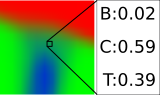
Image	Segmentation	MAP	Prob. map	Prob. values

Figure 3: Poor classification. Maximum a posteriori, MAP, does not separate adjacent cells due to poor probabilities in the junctions shown above. The misclassification of just a few pixels renders a wrong cell topology. Probability maps are shown as RGB images with Background (red), Cell (green) and Touching (blue) classes.

 

\begin{overpic}[width=143.09538pt]{images/map.pdf} \put(14.0,78.0){{\small Maximum A Posterior}} \end{overpic}

\begin{overpic}[width=143.09538pt]{images/TH.pdf} \put(35.0,78.0){{\small Threshold}} \end{overpic}

\begin{overpic}[width=143.09538pt]{images/WT.pdf} \put(35.0,78.0){{\small Watershed}} \end{overpic}

Figure 4: Panoptic Quality (PQ) training values for all methods we compare to $W^{3}$, except COMB, using Maximum a Posteriori (MAP), Thresholded Maps (TH) and Watershed Transform (WT) post-processing. $W^{3}$ converges faster to a better solution.

Panoptic Segmentation Performance. We performed an exploration over the parameter space for the two parameters used in the TH and WT postprocessing methods. Table 1 shows a comparison of different post-processing strategies considering the best combination of parameters for Thresholds (TH) and Watershed (WT). For Mask R-CNN we used the same single threshold TH on the instance probability maps of all boxed cells. We performed watershed WT on each boxed cell region with seeds extracted from the most prominent background and foreground regions in the probability maps. Although Lovász-Softmax seems to be a promising loss function, we believe that the small training dataset and minibatch size negatively influenced its performance. For most values of thresholds used in the TH post-processing, the average combination (COMB) improved the overall result due to the reduction of False Positives (see P05 column). Also, in most cases, our $W^{3}$ approach obtained better SQ values than other methods suggesting a better contour adequacy. Because touching and cell intensity distributions overlap, a softer classification was obtained for these regions. MAP did not achieve the same performance of other approaches (Fig. 3). The behavior in Table 1 remained the same during training as shown in Fig. 4.

  Methods MAP TH WT P05 RQ SQ PQ P05 RQ SQ PQ P05 RQ SQ PQ MRCNN 0.9188 0.8617 0.8002 0.6892 0.9343 0.8767 0.8012 0.7019 0.9343 0.8767 0.8019 0.7026 LSMAX 0.3871 0.3236 0.7455 0.2408 0.4348 0.3119 0.7171 0.2286 0.4000 0.3149 0.7073 0.2237 BWM 0.6756 0.5580 0.8674 0.4858 0.8583 0.8504 0.8769 0.7476 0.8193 0.8405 0.8831 0.7437 U-Net 0.6801 0.5381 0.8418 0.4556 0.8413 0.8508 0.8791 0.7492 0.8708 0.8600 0.8850 0.7621 $W^{3}$(Ours) 0.7384 0.6305 0.8721 0.5513 0.8477 0.8439 0.8994 0.7604 0.9028 0.8775 0.8995 0.7896 COMB(Ours) 0.7587 0.6129 0.8698 0.5351 0.8952 0.8851 0.8908 0.7889 0.8925 0.8759 0.8944 0.7837

Table 1: Metric values for different post processing schemes and segmentation methods. Numbers are average values obtained for the best combination of threshold parameters for both TH and WT post processing methods. Tests were done on 7 images, totaling 138 cells, with 14 clusters containing from 2 to approximately 32 cells. Metric values obtained with TH and WT are higher than those obtained with MAP showing that our post procesing schemes improve results. Overall, our $W^{3}$ and COMB outperform other segmentation methods for almost all metrics, except P05, when thresholding and watershed classification schemes are adopted.

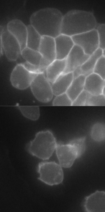
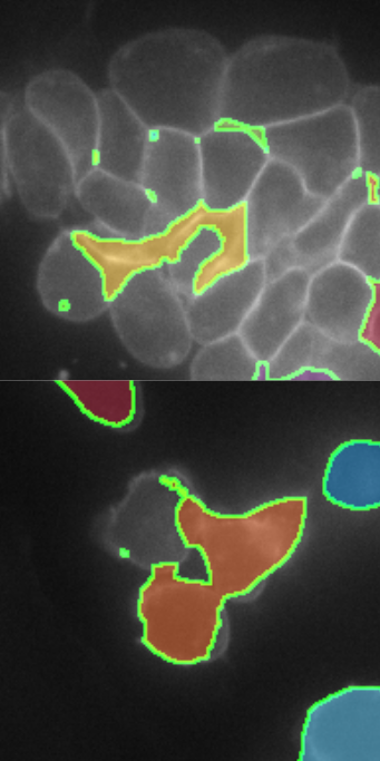
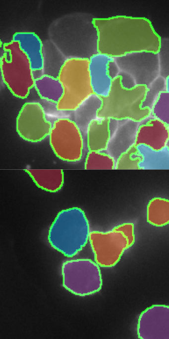
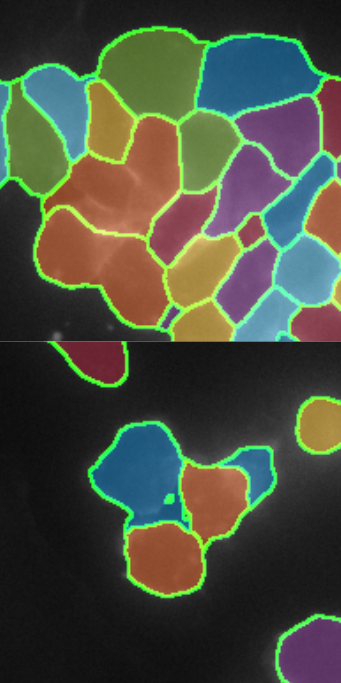
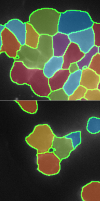
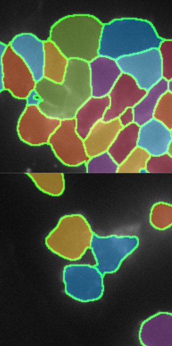
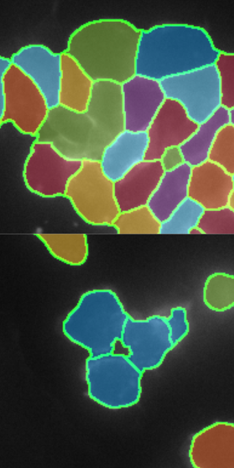
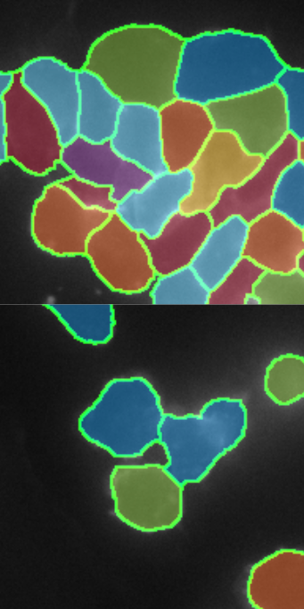
Image	LSMAX	MRCNN	U-Net	BWM	$W^{3}$	COMB	Annotation

Figure 5: Segmentation results for packed cell clusters obtained using methods described in section 3. Colors serve to show cell separation. Note the superiority of our $W^{3}$.

 

\begin{overpic}[width=104.07117pt]{images/fig5a_im.png} \put(25.0,88.0){\color[rgb]{1,1,1}Meristem} \end{overpic}

\begin{overpic}[width=104.07117pt]{images/fig51b_segm.png} \put(15.0,88.0){\color[rgb]{1,1,1}Segmentation} \end{overpic}

\begin{overpic}[width=104.07117pt]{images/fig5c_im.png} \put(35.0,88.0){\color[rgb]{1,1,1}Sepal} \end{overpic}

\begin{overpic}[width=104.07117pt]{images/fig51d_segm.png} \put(15.0,88.0){\color[rgb]{1,1,1}Segmentation} \end{overpic}

Figure 6: Zero-shot panoptic segmentation of meristem and sepal images with our $W^{3}$ method exclusively trained with cell images from different domains.

Examples of segmenting crowded cells with various methods are shown in Fig. 5. In our experiments, MRCNN was able to correctly segment isolated and nearly adjacent cells (second row), but it sometimes failed in challenging high-density clusters. BWM and U-Net tend to misclassify background pixels in neighboring cells (second row) with estimated contours generally beyond cell boundaries. $W^{3}$ had a better detection and segmentation performance with improvement of contour adequacy over COMB.

We believe our combined efforts of data augmentation, loss formulation with per pixel geometric weights, and multiclass classification enabled our trained neural networks to correctly segment cells even from domains it has never seen. For example, we have never trained with images of meristem and sepal cells but we still obtain good quality cell segmentation for these as shown in Fig.6. These solutions might be further improved by training with a few samples from these domains.

4 Conclusions

We proposed a weakly supervised extension to the weighted cross entropy loss function that enabled us to effectively segment crowded cells. We used a semantic approach to solve a panoptic segmentation task with a small training dataset of highly cluttered cells which have incomplete and inaccurate annotations. A new contrast modulation was proposed as data augmentation for touching regions allowing us to perform an adequate panoptic segmentation. We were able to segment images from domains other than the one used for training the network. The experiments showed a better detection and contour adequacy of our method and a faster convergence when compared to similar approaches.

References

- [1] Bai, M., Urtasun, R.: Deep Watershed Transform for Instance Segmentation. In: Proceedings of IEEE CVPR. pp. 5221–5229 (2017)
- [2] Berman, M., Rannen Triki, A., Blaschko, M.B.: The Lovász-Softmax Loss: A Tractable Surrogate for the Optimization of the Intersection-Over-Union Measure in Neural Networks. In: Proceedings of IEEE CVPR. pp. 4413–4421 (2018)
- [3] Glorot, X., Bengio, Y.: Understanding the Difficulty of Training Deep Feedforward Neural Networks. In: Proceedings of 13th AISTATS. pp. 249–256 (2010)
- [4] Guerrero-Pena, F.A., Fernandez, P.D.M., Ren, T.I., Yui, M., Rothenberg, E., Cunha, A.: Multiclass Weighted Loss for Instance Segmentation of Cluttered Cells. In: 2018 25th IEEE ICIP. pp. 2451–2455. IEEE (2018)
- [5] He, K., Gkioxari, G., Dollár, P., Girshick, R.: Mask R-CNN. In: Proceedings of IEEE ICCV. pp. 2961–2969 (2017)
- [6] Kervadec, H.et. al.: Constrained-CNN Losses for Weakly Supervised Segmentation. Medical Image Analysis 54, 88–99 (2019)
- [7] Kirillov, A., He, K., Girshick, R., Rother, C., Dollár, P.: Panoptic Segmentation. arXiv preprint arXiv:1801.00868 (2018)
- [8] Liang, Q., Nan, Y., Coppola, G., Zou, K., Sun, W., Zhang, D., Yu, G.: Weakly-Supervised Biomedical Image Segmentation by Reiterative Learning. IEEE Journal of Biomedical and Health Informatics (2018)
- [9] Ronneberger, O., Fischer, P., Brox, T.: U-Net: Convolutional Networks for Biomedical Image Segmentation. In: MICCAI Conference. pp. 234–241. Springer (2015)
- [10] Schmidt, U., Weigert, M., Broaddus, C., Myers, G.: Cell Detection with Star-Convex Polygons. In: MICCAI Conference. pp. 265–273. Springer (2018)
- [11] Yang, L., Zhang, Y., Chen, J., Zhang, S., Chen, D.Z.: Suggestive Annotation: A Deep Active Learning Framework for Biomedical Image Segmentation. In: MICCAI Conference. pp. 399–407. Springer (2017)