A Quantum Ring in a Nanosphere

Abstract

In this paper we study the quantum dynamics of an electron/hole in a two-dimensional quantum ring within a spherical space. For this geometry, we consider a harmonic confining potential. Suggesting that the quantum ring is affected by the presence of an Aharonov-Bohm flux and an uniform magnetic field, we solve the Schrödinger equation for this problem and obtain exactly the eigenvalues of energy and corresponding eigenfunctions for this nanometric quantum system. Afterwards, we calculate the magnetization and persistent current are calculated, and discuss influence of curvature of space on these values.

I Introduction

In recent years, the study of confined quasiparticles in nanostructures with annular geometry has attracted great interest in condensed matter physics. These quantum rings exhibit several interesting physical phenomena, such as the Aharonov-Bohm effect 9 ; 10 , spin-orbit interaction effects spin , persistent currents 12 ; 13 , quantum Hall effect 11 and the manifestation of Berry geometric quantum phase 14 . More recent works have demonstrated that assumption of finite width brings intricacy from an experimental point of view, although even more important results have been also found. So, in Ref. lorke it was shown through use of experiments with quantum rings of very small radii containing few electrons, that there are some electron modes representing different radii of electronic orbits in these nanometric systems. Several results show that magnetic field penetration depth in a conducting region plays an important role for physical properties of finite width quantum rings, including multiple channels which were experimentally observed 12 ; 13 ; inkson ; margulis ; bogachek . One-dimensional quantum rings pierced by Aharonov-Bohm solenoid were used to observe the quantum interference effect spin ; 14 ; 15 ; 16 . There are several exactly solvable models known for two-dimensional quantum rings, for example, those ones considered in refs. 12 ; inkson ; margulis ; bogachek . The theoretical approach developed by Tan and Inkson inkson ; 12 is of a special interest since it presents good agreement with experimental results, for instance, concerning effects of magnetic field penetration in the conducting region.

Landau levels in negative dune ; comtet ; comtet1 and positive dune ; greiter curvature cases have been intensively studied in order to explore quantum Hall effect in these spaces bulaphysb ; takuya ; jelal ; iengo ; nair ; hasebe . Quantum Hall effect in a Lobachevsky plane was considered in ref. bulaphysb , where the effect of negative curvature was observed for a Hall conductivity of these systems. The study of quantum Hall effect in a spherical space was carried out for different scenarios in Refs. hasebe2 ; nair2 ; nair3 ; nair3 ; nair4 . Advances in the development of techniques for low dimensional materials motivate many investigations concerning curvature and topology influence on nanostructures, since now it is possible to obtain several kinds of curved two-dimensional surfaces 16 and objects of nanometric size with desired shapes prinz . The impacts of curvature and topology for magnetic, spectral and transport properties of nanostructured materials have recently been studied by several authors 17 ; 18 ; 19 ; 20 . The magnetic moment of two-dimensional electron gas on a negative curvature surface was studied in ref. bulaemag . The effect of a negative curvature for a quantum dot with impurity was investigated in ref. geyler . The zero mode in systems for spin-$1/2$ particle in the presence of an Aharonov-Bohm solenoid in Lobachevsky plane was obtained in ref. geyler1 . Recently, Bulaev, Geyler and Margulis  bulacurva have studied the Tan-Inkson model 12 ; inkson in hyperbolic spaces and provided theoretical frameworks, comprising potentials with adjustable parameters, capable of describing nanostructures like quantum dots, antidots, rings and wires in this surface of negative curvature. Recently the effect of topology in quantum rings and dots was investigated in the refs. 22 ; 23 ; lincoan .

In this work we study a nanosystem in a positive curvature case. This case is interesting, among other reasons, because of the characteristics of the growth techniques for nanometric systems, such as quantum rings. Therefore, we have a motivation for probing how curvature influences physical properties of quantum rings. In our work we study a nanometric system grown over a surface with positive curvature, more specifically, a quantum ring in a spherical space in the presence of an Aharonov-Bohm flux and an uniform magnetic field through that space. We obtain the spectrum of energy and the wave function for Schrödinger equation solved exactly for this system. The magnetization in the zero temperature case is obtained, and the influence of curvature on the magnetization is investigated. The persistent current is obtained using the Byers-Yang relation byers , and the influence of curvature on it is discussed. An uniform magnetic field in this case is introduced through the curved space in order to observe what happens in the conducting region. We also compare our results in the appropriated limit with results obtained in Ref. bulacurva for a ring on a negative curvature surface.

This paper is organized as follows. In Section II we investigate the quantum dynamics in a two-dimensional spherical space. In Section III, we describe the confinement potential for this positive curvature space. In Section IV the quantum dynamics of a charged particle confined in a Tan-Inkson potential is investigated and the eigenvalues and eigenvectors of energy are obtained. In Section V the magnetization for $T=0$ is found and the physical properties is discussed. The persistent current is f calculated in Section VI. Finally, in Section VII we present the concluding remarks.

II Quantum dynamics in a two-dimensional spherical space

First of all, we write the Hamiltonian for a free particle in a two-dimensional space $S^{2}$ described by a sphere embedded in the Euclidean three-dimensional space, $x^{2}+y^{2}+z^{2}=a^{2}$, where $a$ is the radius of sphere. In this case the metric on the sphere, in terms of angular coordinates $(\theta,\varphi)$ and sphere radius $a$, is given by

$$ds^{2}=a^{2}d\theta^{2}+a^{2}\sin^{2}\theta d\varphi^{2},$$ (1)

where angular coordinates are restricted to the range $0<\theta<\pi$ and $0<\varphi<2\pi$. In this study we use a stereographic projection from the points in a sphere with radius $a$ on a plane. It is worth noting that the stereographic projection is a kind of map preserving angles and circles. In this way, first, angles between curves on original space are mapped into equal angles comprised by respective curves on projected plane; second, image of a circle on the original space is also a circle on the projected space. After this process, the points are at the distance $\rho$ from the origin (that is, from the sphere’s center) on the projection plane. Here the zenith angle is denoted by $\theta$ (which corresponds to the $\psi$ angle in the Figure (1).

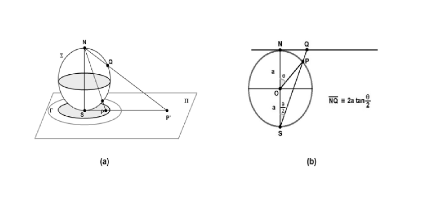
Figure 1: (a) Stereographic projection of a sphere on a plane. (b) Trigonometric relation useful for obtaining the metric for the projected space.

In this way, we obtain the following relations:

$$\tan\frac{\theta}{2}=\frac{\rho}{2a}\quad,$$ (2)

and

$$d\theta^{2}=\frac{1}{a^{2}\left[1+\left(\frac{\rho}{2a}\right)^{2}\right]^{2}}d\rho^{2}\quad,$$ (3)

and after some algebra we find the metric describing our stereographically projected system:

$$ds^{2}=\frac{d\rho^{2}+\rho^{2}d\varphi^{2}}{\left[1+\left(\frac{\rho}{2a}\right)^{2}\right]^{2}}\ ,$$ (4)

where $0<\rho<\infty$ and $0<\varphi<2\pi$. We will consider an uniform magnetic field $B$ on the spherical surface. So, for the projected representation, the equivalent magnetic field will be along the $z$-direction, perpendicular to the projection plane. The vector potential for this field configuration for the geometry described by (4) is given by

$$\vec{A_{1}}=\left(0,\frac{B\rho}{2\left[1+\left(\frac{\rho}{2a}\right)^{2}\right]^{2}}\right).$$ (5)

Now, we introduce a Aharonov-Bohm magnetic flux ($\Phi_{AB}$) Landau:hydrogen3 ; sakurai ; bogachek ; Furtado:density ; Dunne in $z$-direction on the sphere. Therefore, the only non-vanishing component of the magnetic vector potential is the azimuthal one, and the corresponding vector potential is $\vec{A_{2}}$ given by

$$\vec{A_{2}}=\left(0,\frac{\Phi_{AB}}{2\pi\rho}\right).$$ (6)

The Hamiltonian in the curved space characterized by the metric $g_{ij}$ in the presence of external magnetic fields is given by

$$H_{0}=\frac{1}{2\mu\sqrt{g}}\left(-i\hbar\frac{\partial}{\partial x^{i}}-\frac{e}{c}A_{i}\right)\sqrt{g}g^{ij}\left(-i\hbar\frac{\partial}{\partial x^{j}}-\frac{e}{c}A_{j}\right).$$ (7)

Hence, the Hamiltonian (7) in the space with the metric (4) looks like

$$\begin{split}\hat{H_{0}}\,=\,-\frac{\hbar^{2}}{2\mu a^{2}}\left\{a^{2}\left[1+\left(\frac{\rho}{2a}\right)^{2}\right]^{2}\left[\frac{1}{\rho}\frac{d}{d\rho}\left(\rho\frac{d}{d\rho}\right)+\frac{1}{\rho^{2}}\left(\frac{\partial}{\partial\varphi}+i\frac{\Phi_{AB}}{\Phi_{0}}\right)\right]\right\}\,\\ -\,i\frac{\hbar\omega_{c}}{2}\left[1+\left(\frac{\rho}{2a}\right)^{2}\right]\left(\frac{\partial}{\partial\varphi}+i\frac{\Phi_{AB}}{\Phi_{0}}\right)+\frac{\mu\omega_{c}^{2}\left(-a^{2}\right)}{2}\left(\frac{\rho}{2\left(ia\right)}\right)^{2}\,+\,\frac{\hbar^{2}}{8\mu a^{2}}\,.\end{split}$$ (8)

This operator describes a quantum particle in a two-dimensional spherical space submitted to an uniform magnetic field, in the presence of Aharonov-Bohm solenoid in $z$-direction.

III The Tan-Inkson Confinement Potential in a Two-dimensional Spherical Space

Let us introduce a confinement potential in a two-dimensional spherical space $S^{2}$. We generalize the Tan-Inkson inkson potential for this geometry. This potential is a harmonic confining potential describing different kinds of nanostructures in a spherical space, after a simple change of parameters, is given by

$$V(\rho)=\lambda_{1}\rho^{2}+\frac{\lambda_{2}}{\rho^{2}}\left[1+\left(\frac{\rho}{2a}\right)^{2}\right]^{2}-V_{0},$$ (9)

where $\lambda_{1}$ and $\lambda_{2}$ are the parameters of the potential and $V_{0}$ looks like

$$V_{0}=\frac{\lambda_{2}}{2a^{2}}+2\sqrt{\lambda_{2}\left(\lambda_{1}+\frac{\lambda_{2}}{\left(2a\right)^{4}}\right)}.$$ (10)

The potential (9) has a minimum in $\rho_{0}$ equal to

$$\rho_{0}=\left(\frac{\lambda_{2}}{\lambda_{1}+\frac{\lambda_{2}}{(2a)^{4}}}\right)^{1/4}.$$ (11)

It is worth noting that, in the limit of $\lambda_{2}\to 0$ for the potential presented by (9), in stereographic coordinates, one recovers the harmonic potential for a quantum dot in a flat space. Besides, if we consider this system in the spherical coordinates characterizing the metric (4), the quantum dot takes the form $V(\theta)=4\lambda_{1}a^{2}\tan^{2}(\theta)$. For the case $\lambda_{2}\to 0$, we arrive at the antidot potential in spherical space. In the limit $a\to\infty$, we obtain the flat Tan-Inkson potential in the form

$$V(\rho)=\lambda_{1}\rho^{2}+\frac{\lambda_{2}}{\rho^{2}}-V_{0},$$ (12)

where $V_{0}$ is given by

$$V_{0}=2\sqrt{\lambda_{2}\lambda_{1}}.$$ (13)

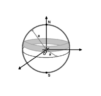
Figure 2: Quantum ring on sphere

IV The quantum Dynamics in a Quantum Ring in Spherical Space

Now we solve the Schrödinger equation for an electron/hole confined by the potential (9), in the presence of magnetic fields (5) and (6). In this case the Hamiltonian of an electron is given by

$$\begin{split}\hat{H}\,=\,-\frac{\hbar^{2}}{2\mu a^{2}}\left\{a^{2}\left[1+\left(\frac{\rho}{2a}\right)^{2}\right]^{2}\left[\frac{1}{\rho}\frac{d}{d\rho}\left(\rho\frac{d}{d\rho}\right)+\frac{1}{\rho^{2}}\left(\frac{\partial}{\partial\varphi}+i\frac{\Phi_{AB}}{\Phi_{0}}\right)\right]\right\}\,\\ -\,i\frac{\hbar\omega_{c}}{2}\left[1+\left(\frac{\rho}{2a}\right)^{2}\right]\left(\frac{\partial}{\partial\varphi}+i\frac{\Phi_{AB}}{\Phi_{0}}\right)+\frac{\mu\omega_{c}^{2}\left(-a^{2}\right)}{2}\left(\frac{\rho}{2\left(ia\right)}\right)^{2}\,+\,\frac{\hbar^{2}}{8\mu a^{2}}\,\\ +\,\lambda_{1}\rho^{2}\,+\,\frac{\lambda_{2}}{\rho^{2}}\left[1+\left(\frac{\rho}{2a}\right)^{2}\right]^{2}\,-\,V_{0}\,.\end{split}$$ (14)

We must solve the Schrödinger equation $\hat{H}\Psi(\rho,\varphi)=E\Psi(\rho,\varphi)$. To do it, first we make the following change of the variable

$$x\equiv\frac{1}{1\,+\,\left(\frac{\rho}{2a}\right)^{2}}\,.$$ (15)

Substituting this in (14), we obtain the following equation

$$\begin{split}-\frac{\hbar^{2}}{2\mu a^{2}}\left\{a^{2}\frac{1}{x^{2}}\left[\frac{1}{a^{2}}\left(x^{2}\frac{d}{dx}\left[x(1-x)\right]\frac{d}{dx}\right)-\frac{1}{4a^{2}}\left(\frac{x}{1-x}\right)\left(\frac{\partial}{\partial\varphi}+i\frac{\Phi_{AB}}{\Phi_{0}}\right)\right]\right\}\Psi(x,\varphi)\,\\ -\,i\frac{\hbar\omega_{c}}{2}\frac{1}{x}\left(\frac{\partial}{\partial\varphi}+i\frac{\Phi_{AB}}{\Phi_{0}}\right)\Psi(x,\varphi)+\frac{\mu\omega_{c}^{2}a^{2}}{2}\left(\frac{1-x}{x}\right)\Psi(x,\varphi)\,+\,\frac{\hbar^{2}}{8\mu a^{2}}\Psi(x,\varphi)\\ +\lambda_{1}\,4a^{2}\,\left(\frac{1-x}{x}\right)\Psi(x,\varphi)\,+\,\lambda_{2}\,\frac{1}{4a^{2}}\left(\frac{x}{1-x}\right)\frac{1}{x^{2}}\Psi(x,\varphi)\,-\frac{\lambda_{2}}{2a^{2}}\Psi(x,\varphi)-\\ -\,\frac{\mu}{4}\omega_{0}^{2}\Psi(x,\varphi)\,\rho_{0}^{2}\,=E\Psi(x,\varphi).\end{split}$$ (16)

From (16), using the ansatz $\Psi\left(\rho,\,\varphi\right)\,=\,\frac{e^{i\,m\varphi}}{\sqrt{2\pi}}\,f_{m}(x)$, we obtain the following Schrödinger equation

$$\begin{split}-\frac{\hbar^{2}}{2\mu a^{2}}\left\{\frac{1}{x^{2}}\left[x^{2}\,\frac{d}{dx}(x(1-x))\frac{d}{dx}\,-\,\frac{1}{4}\left(\frac{x}{1-x}\right)\left(m\,+\,\frac{\Phi_{AB}}{\Phi_{0}}\right)^{2}\right]\right\}\,f_{m}(x)\\ +\,\frac{\hbar\omega_{c}}{2}\left(m\,+\,\frac{\Phi_{AB}}{\Phi_{0}}\right)\,\frac{1}{x}\,f_{m}(x)\\ +\,\left\{\frac{\mu\,\omega_{c}^{2}\,a^{2}}{2}\frac{1}{x}\,-\,\frac{\mu\,\omega_{c}^{2}\,a^{2}}{2}\,+\,\frac{\hbar^{2}}{8\mu a^{2}}\,+\,\frac{\left[\frac{1}{2}\mu\,a^{2}\,\omega_{0}^{2}\,-\,\frac{1}{2}\,\mu\,a^{2}\,\omega_{0}^{2}\left(\frac{\rho_{0}}{2a}\right)^{4}\right]\,x}{1-x}\,+\,\frac{\frac{\mu\,a^{2}\,\omega_{0}^{2}}{2}}{x(1-x)}\right\}\,f_{m}(x)\\ -\left\{\,\frac{\left[\mu\,a^{2}\,\omega_{0}^{2}\,-\,\mu\,a^{2}\,\omega_{0}^{2}\left(\frac{\rho_{0}}{2a}\right)^{4}\right]}{1-x}\,+\,\mu\,a^{2}\,\omega_{0}^{2}\left(\frac{\rho_{0}}{2a}\right)^{4}\,+\,\frac{\mu}{4}\,\omega_{0}^{2}\,\rho_{0}^{2}\right\}\,f_{m}(x)=\,E\,f_{m}(x)\,,\end{split}$$ (17)

where $\omega_{c}=\frac{eB}{m}$ is a cyclotron frequency and

$$\omega_{0}=\sqrt{\frac{8}{\mu}\left[\lambda_{1}+\frac{\lambda_{2}}{\left(2a\right)^{4}}\right]}\quad.$$ (18)

Now, after some algebra we obtain

$$\begin{split}\left\{-\frac{d}{dx}(x(1-x))\frac{d}{dx}\,+\,\frac{M^{2}}{4}\frac{1}{1-x}\,+\,\frac{\mu^{2}a^{4}}{\hbar^{2}}\omega_{m}^{2}\frac{1}{x}\,-\,\frac{\mu^{2}a^{4}}{\hbar^{2}}\left[\omega_{c}^{2}\,+\,\omega_{0}^{2}\left(1\,+\,\left(\frac{\rho_{0}}{2a}\right)^{2}\right)^{2}\right]\right\}f_{m}(x)\\ =\,\left\{\frac{2\mu a^{2}}{\hbar^{2}}\,E\,-\,\frac{1}{4}\right\}f_{m}(x)\end{split}$$ (19)

where

$$M\equiv\sqrt{\left(m\,+\,\frac{\Phi_{AB}}{\Phi_{0}}\right)^{2}\,+\,\left(\frac{\mu\omega_{0}\rho_{0}^{2}}{2\hbar}\right)^{2}}\,,$$ (20)

$$\omega_{m}\equiv\sqrt{\left(\omega_{c}\,+\,\frac{\hbar}{2\mu a^{2}}\left(m\,+\,\frac{\Phi_{AB}}{\Phi_{0}}\right)\right)^{2}\,+\,\omega_{0}^{2}},$$ (21)

$$E^{\prime}\,=\,\frac{2\mu a^{2}}{\hbar^{2}}\,E.$$ (22)

Thus, rearranging terms in (19), we write

$$\begin{split}\left\{\frac{d^{2}}{dx^{2}}\,+\,\left(\frac{1}{x}\,-\,\frac{1}{1-x}\right)\frac{d}{dx}\,+\,\left[\frac{-\frac{\mu^{2}a^{4}\omega_{m}^{2}}{\hbar^{2}}}{x}\,+\,\frac{-\frac{M^{2}}{4}}{1-x}\right]\frac{1}{x(1-x)}\right\}f_{m}(x)\\ -\,\left\{\frac{1}{4}-\frac{2\mu a^{2}}{\hbar^{2}}E\,-\,\frac{\mu^{2}a^{4}}{\hbar^{2}}\left[\omega_{c}^{2}\,+\,\omega_{0}^{2}\left(1\,+\,\left(\frac{\rho_{0}}{2a}\right)^{2}\right)^{2}\right]\right\}\frac{1}{x(1-x)}f_{m}(x)=\,0.\end{split}$$ (23)

The equation (23) replays the form of following differential equation

$$\frac{d^{2}\,P(\xi)}{d\xi^{2}}\,+\,\left(\frac{1-\alpha-\alpha^{\prime}}{\xi}\,-\,\frac{1-\gamma-\gamma^{\prime}}{1-\xi}\right)\frac{d\,P(\xi)}{d\xi}\,+\,\left(\frac{\alpha\,\alpha^{\prime}}{\xi}\,-\,\frac{\gamma\,\gamma^{\prime}}{1-\xi}\,-\,\beta\,\beta^{\prime}\right)\times$$ (24)

$$\times \frac{1}{\xi\left(\xi-1\right)}P(\xi)\,=\,0\,,$$

where

$$\alpha\,+\alpha^{\prime}\,+\,\beta\,+\,\beta^{\prime}\,+\,\gamma\,+\gamma^{\prime}\,=\,1\,.$$ (25)

It is important to note that (24) and (25) are similar to Eqs. ($5$) and ($5a$) in Ref. rubino . Further, we can see that (24) has the form of the hypergeometric equation, whose solution reads as

$$P(\xi)\,=\,\xi^{\alpha}\,\left(1-\xi\right)^{\gamma}\,F\left(a^{\prime},b^{\prime},c^{\prime};\xi\right)\,,$$ (26)

where

$$a^{\prime}\,=\,\alpha\,+\,\beta\,+\,\gamma,\quad b^{\prime}\,=\,\alpha\,+\,\beta^{\prime}\,+\,\gamma,\quad c^{\prime}\,=\,1\,+\,\alpha\,-\,\alpha^{\prime}\,.$$ (27)

Comparing (24) and (23), we see that

$$1\,-\,\alpha\,-\,\alpha^{\prime}\,=1\quad\to\alpha\,=\,-\alpha^{\prime}.$$ (28)

and at the same way

$$\gamma\,=\,-\gamma^{\prime}\quad\mbox{and}\quad\beta^{\prime}\,=\,1\,-\,\beta\,.$$ (29)

Let us define

$$\alpha\equiv\frac{\mu a^{2}}{\hbar}\,\omega_{m}\,,$$ (30)

and

$$\gamma\equiv\frac{M}{2}\,.$$ (31)

We can also use the relation

$$\beta\,\left(1\,-\,\beta\right)\,=\,\frac{1}{4}\,-\,\frac{2\mu a^{2}}{\hbar^{2}}E\,-\,\frac{\mu^{2}a^{4}}{\hbar^{2}}\left[\omega_{c}^{2}\,+\,\omega_{0}^{2}\left(1\,+\,\left(\frac{\rho_{0}}{2a}\right)^{2}\right)^{2}\right]\,.$$ (32)

From last relations it is easy to see that we can assume

$$P(x)\,=\,x^{\alpha}\,\left(1\,-\,x\right)^{\gamma}\,F\left(\alpha\,+\,\beta\,+\,\gamma,\,\alpha\,+\,\gamma\,+\,1\,-\,\beta,\,1\,+\,2\alpha,\,x\right)\,.$$ (33)

From (32) we find the following expression

$$\beta\,=\,\frac{1}{2}\,\pm\,\sqrt{\frac{2\mu a^{2}}{\hbar^{2}}E\,+\,\frac{\mu^{2}a^{4}}{\hbar^{2}}\omega_{c}^{2}\,+\,\frac{\mu^{2}a^{4}}{\hbar^{2}}\omega_{0}^{2}\,+\,2\frac{\mu^{2}a^{4}}{\hbar^{2}}\omega_{0}^{2}\left(\frac{\rho_{0}}{2a}\right)^{2}\,+\,\frac{\mu^{2}a^{4}}{\hbar^{2}}\omega_{0}^{2}\left(\frac{\rho_{0}}{2a}\right)^{4}}.$$ (34)

Assuming, because of (33), that

$$\alpha\,+\,\beta\,+\,\gamma\,\leqslant\,-n\,$$ (35)

and considering (30), (31) and (34), and solving condition (35) when equality holds, after some algebra and substituting the explicit values for $\alpha,\,\beta,\,\gamma,\,\omega_{m}^{2},\,M^{2}$, basing on previously obtained relations, we obtain the following energy eigenvalues

$$\begin{split}E\,=\,\frac{\hbar^{2}}{2\mu a^{2}}\left[\left(n\,+\,\frac{1}{2}\right)^{2}\,+\,\left(n\,+\,\frac{1}{2}\right)M\,+\,\frac{1}{2}\left(m\,+\,\frac{\Phi_{AB}}{\Phi_{0}}\right)^{2}\right]\,+\,\hbar\,\omega_{m}\left(n\,+\,\frac{1}{2}\,+\,\frac{M}{2}\right)\\ +\,\hbar\,\omega_{c}\left(m\,+\,\frac{\Phi_{AB}}{\Phi_{0}}\right)\,-\,\frac{\mu\omega_{0}^{2}\rho_{0}^{2}}{4},\end{split}$$ (36)

with $n\,\in\,\mathbb{N}:\,0\,\leqslant\,n\,<\,\frac{\mu\omega_{m}a^{2}}{\hbar}\,-\,\frac{M}{2}\,-\,\frac{1}{2}$ . In the limit $\lambda_{1}=\lambda_{2}=0$ and $\Phi_{AB}=0$ we find the results obtained by Dunne Dunne for Landau levels in a spherical space. Here we can see that eigenvalues are only discrete, in contrast with the case of hyperbolic space where the Landau levels are studied in Refs. comtet ; comtet1 ; Dunne and the eigenvalues can be discrete as well as and continuous. In the limit $a\to\infty$ we recover the results obtained by Tan and Inkson 12 given by

$$E=\hbar\,\omega_{fm}\left(n\,+\,\frac{1}{2}\,+\,\frac{M}{2}\right)+\hbar\,\omega_{c}\left(m\,+\,\frac{\Phi_{AB}}{\Phi_{0}}\right)\,-V_{0}$$ (37)

where flat definition $V_{0}$ is given by Eq. (13), and $\omega_{fm}=\sqrt{(\omega_{c}^{2}+\omega_{0})^{2}}$.

V The Magnetization for Quantum Ring in Spherical space

Considering our system as a canonical ensemble, one can obtain the magnetization landau-stat , from a Helmholtz free energy and a magnetic field, as

$$\mathcal{M}(B)\,=\,-\left(\frac{\partial F}{\partial B}\right)_{T,N}\,=\,{\sum}_{n,m}\mathcal{M}_{n,m}\,f_{0}\left(E_{n,m}\right)\,$$ (38)

where $N$ represents the number of electrons and $f_{0}$ is the Fermi distribution function. In this case, magnetic moment for each $(n,m)$th state is given by

$$\mathcal{M}_{n,m}\,=\,-\frac{\partial E_{n,m}}{\partial B},$$ (39)

with

$$N\,=\,{\sum}_{n,m}\,f_{0}\left(E_{n,m}\right).$$ (40)

Noting that $\omega_{m}$ depends on the magnetic field $B$, $\omega_{c}$, one can write

$$\frac{\partial}{\partial B}\,=\,\frac{\partial\omega_{c}}{\partial B}\,\frac{\partial}{\partial\omega_{c}},$$ (41)

which implies the following relation

$$\mathcal{M}_{n,m}\,=\,-\frac{e}{\mu c}\,\frac{\partial}{\partial\omega_{c}}\,E_{n,m}.$$ (42)

In this way, we can use the above relation and the energy eigenvalues (36), and obtain

$$\mathcal{M}_{n,m}\,=\,\mu_{B}\frac{m_{0}}{\mu}\left[\hbar\left(2n+M+1\right)\frac{\partial}{\partial\omega_{c}}\omega_{m}\,+\,\left(m+\frac{\Phi_{AB}}{\Phi_{0}}\right)\right],$$ (43)

where $m_{0}$ represents the electron rest mass and $\mu_{B}$ is Bohr magneton given by

$$\mu_{B}\,=\,\frac{e\,\hbar}{2m_{0}c}.$$ (44)

Taking into account that

$$\frac{\partial}{\partial\omega_{c}}\omega_{m}\,=\,\frac{1}{\omega_{m}}\left[\omega_{c}\,+\,\frac{\hbar}{2\mu a^{2}}\left(m+\frac{\Phi_{AB}}{\Phi_{0}}\right)\right],$$ (45)

finally we find

$$\frac{\mathcal{M}_{n,m}}{\mu_{B}}\,=\,-\frac{m_{0}}{\mu}\,\left[\left(2n\,+\,M\,+\,1\right)\frac{\omega_{c}\,+\,\frac{\hbar\left(m+\frac{\Phi_{AB}}{\Phi_{0}}\right)}{2\mu a^{2}}}{\omega_{m}}\,+\,m+\frac{\Phi_{AB}}{\Phi_{0}}\right].$$ (46)

The expression (46) is the magnetization for $T=0$ for a two-dimensional quantum ring in a spherical space. Applying limit $a\to\infty$, we recover the flat case 12 ; footnote1 for Gaussian CGS units.

VI The Persistent current in Quantum Ring in Spherical Space

In this section we investigate the arising of the persistent current in a two-dimensional quantum ring for the spherical geometry. Then, we also obtain persistent currents from (36). It was showed in byers-yang that for known energy eigenvalues, we can obtain the current from the following relation

$$I_{n,m}\,=\,-c\,\frac{\partial E_{n,m}}{\partial\Phi_{AB}},\,$$ (47)

that is, the Byers-Yang relation. In this way, the persistent currents will be given by

$$\begin{split}I_{n,m}\,=\,-c\left\{\frac{\hbar^{2}}{2\mu a^{2}}\left[\left(n+\frac{1}{2}\right)\frac{\partial M}{\partial\Phi_{AB}}\,+\,\frac{1}{2}\frac{\partial}{\partial\Phi_{AB}}\,\left(m+\frac{\Phi_{AB}}{\Phi_{0}}\right)^{2}\right]\,+\,\hbar\left(n+\frac{1}{2}+\frac{M}{2}\right)\frac{\partial\omega_{m}}{\partial\Phi_{AB}}\right\}\\ \,-\frac{c}{2}\hbar\omega_{m}\frac{\partial M}{\partial\Phi_{AB}}\,-\,c\,\frac{\hbar\omega_{c}}{2}\frac{1}{\Phi_{0}}\,.\end{split}$$ (48)

Taking into account that

$$\frac{\partial M}{\partial\Phi_{AB}}\,=\,\frac{1}{2}\,\frac{1}{M}\,2\,\left(m+\frac{\Phi_{AB}}{\Phi_{0}}\right)\,\frac{1}{\Phi_{0}}\,=\,\frac{1}{M}\left(m+\frac{\Phi_{AB}}{\Phi_{0}}\right)\,\frac{1}{\Phi_{0}}\,,$$ (49)

and

$$\frac{\partial\omega_{m}}{\partial\Phi_{AB}}\,=\,2\,\left(m+\frac{\Phi_{AB}}{\Phi_{0}}\right)\,\frac{1}{\Phi_{0}}\,=\,\frac{\partial\omega_{m}}{\partial\Phi_{AB}}\,=\,\frac{\hbar}{2\mu a^{2}}\,\frac{1}{\Phi_{0}}\,\left[\frac{\omega_{c}\,+\,\frac{\hbar}{2\mu a^{2}}\left(m+\frac{\Phi_{AB}}{\Phi_{0}}\right)}{\omega_{m}}\right]\,,$$ (50)

and substituting (49) and (50) in (48), one finds

$$\begin{split}I_{n,m}\,=\,(-c)\left\{\left[\frac{\hbar^{2}}{2\mu a^{2}}\frac{\left(2n+1\right)}{2}\,+\,\frac{\hbar\omega_{m}}{2}\right]\frac{1}{\Phi_{0}}\frac{1}{M}\left(m+\frac{\Phi_{AB}}{\Phi_{0}}\right)\,+\,\frac{\hbar^{2}}{2\mu a^{2}}\left(m+\frac{\Phi_{AB}}{\Phi_{0}}\right)\frac{1}{\Phi_{0}}\right\}\\ -c\left\{\frac{\hbar}{2}\left(2n+M+1\right)\frac{\hbar}{2\mu a^{2}}\frac{1}{\Phi_{0}}\left[\frac{\omega_{c}\,+\,\frac{\hbar}{2\mu a^{2}}\left(m+\frac{\Phi_{AB}}{\Phi_{0}}\right)}{\omega_{m}}\right]\,+\,\frac{\hbar\omega_{c}}{2}\frac{1}{\Phi_{0}}\right\}\,.\end{split}$$ (51)

Here we used

$$\Phi_{0}\,\equiv\,\frac{hc}{e}\,=\,\frac{2\pi\hbar c}{e}\,,$$ (52)

where $e$ is the electron/hole charge. After some algebraic manipulations we obtain

$$I_{n,m}\,=\,\frac{c}{\pi\rho_{m}^{2}}\left\{\mathcal{M}_{n,m}\left[1+\left(\frac{\rho_{m}}{2a}\right)^{2}\right]\,+\,\mu_{B}\frac{m_{0}}{\mu}\frac{\omega_{c}}{\omega_{m}}\left(2n+1\right)\right\}\,,$$ (53)

where

$$\rho_{m}\,\equiv\,\sqrt{\frac{2\hbar M}{\mu\omega_{m}}}\,,$$ (54)

is the effective radius of the state with a quantum number $m$.

VII Concluding remarks

In this paper we have investigated the two-dimensional quantum ring in the presence of the Aharonov-Bohm quantum flux and an uniform magnetic field in the spherical space. We obtained the eigenvalues and eigenfunctions of the Hamiltonian and demonstrated the influence of curvature on these physical quantities. We have found the magnetization and the persistent current for $T=0$ and showed the influence of the curvature on these cases. In the zero curvature limit ($a\to\infty$) we reproduced the previous results obtained by Tan and Inkson 12 . In the case where $\lambda_{1}=\lambda_{2}=0$ and $\Phi_{AB}=0$ we obtained the Landau levels in spherical space Dunne . Notice that in the expression (53) the first contribution is caused by the classical current in a quantum ring of radius $\rho_{m}$ exposed to a magnetic field, the second contribution arises due to the magnetic field penetration in the conduction region of the two-dimensional ring, and this contribution is responsible for breaking the proportionality of the magnetic moment and the persistent current, a similar case was observed by Bulaev et al. for a two-dimensional quantum ring in hyperbolic space bulaphysb . In the limit $\omega_{c}<<\omega_{0}$ the current is proportional to the magnetic moment. We can write the magnetization in the following way:

$$\mathcal{M}_{n,m}=\left\{\frac{c\pi\rho_{m}^{2}}{\left[1+\left(\frac{\rho_{m}}{2a}\right)^{2}\right]}I_{n,m}\,-\,\mu_{B}\frac{m_{0}}{\mu}\frac{\omega_{c}}{\omega_{m}}\left(2n+1\right)\right\}\,.$$ (55)

It follows from Eq. (55) that the magnetization can be presented as a sum of two terms. The first one arises due to a magnetic dipole moment of a current loop within spherical geometry, and in the limit $a\to\infty$ we recover the classical results  jackson . The another contribution corresponds to a diamagnetic shift. This term has a contribution due to the curvature dependence in the term $\frac{\omega_{c}}{\omega_{m}}$. Finally, we claim that with the development on nanotechnology the possibility to investigate this spherical system from the experimental point of view can be realized technically which can allow to obtain this spherical thin shell material . We emphasize the interest to investigating the spherical systems taken place in recent years, see f.e jelal ; nair ; hasebe ; hasebe2 ; nair2 ; nair3 .

We can use the geometry of the quantum ring in spherical shell to construct an experimental set-up to investigate the physical properties obtained here for this theoretical model. A nanometric system for a quantum ring on a sphere can be experimentally constructed between two well-determined $\theta$ angles in a quasi-two-dimensional nanostructured hemisphere. Electron or holes may be injected by terminals attached to the ring and the persistent current can be measured in this experimental scheme similar to that described in reference Ref.gao For flat case. Other properties of these systems that can be investigated in a future publication, such as, de Haas- van Alphen effect and a more detailed numerical study of the contribution of the persistent current and magnetization obtained in previous sections to a system with many particles for $T=0$ and $T\neq 0$.

References

• (1) Y. Aharonov and D. Bohm, Phys. Rev. 115, 485 (1959).
• (2) U. F. Keyser et al, Semicond. Sci. Technol. 17, L22 (2002).
• (3) Y. Meir, O. Entin-Wohlman, Y. Gefen, Phys. Rev. B 42, 8351 (1990).
• (4) W. C. Tan and J. C. Inkson, Phys. Rev. B 60, 5626 (1999).
• (5) Y. Avishai, Y. Hatsugai, and M. Kohmoto, Phys. Rev. B 47, 9501 (1993).
• (6) B. I. Halperin, Phys. Rev. B 25, 2185 (1982).
• (7) V. Chandrasekhar et. al, Phys. Rev. Lett. 67, 3578 (1991).
• (8) A. Lorke, R. J. Luyken, A. O. Govorov, J. P. Kotthaus, J. M. Garcia, and P. M. Petroff, Phys. Rev. Lett. 84, 2223 (2000).
• (9) W. C. Tan and J. C. Inkson, Semicond. Sci. and Technol. 11, 1635 (1996).
• (10) V. A. Margulis, A. V. Shorokhov, and M. P. Trushin, Physica E 10, 518 (2001).
• (11) E. N. Bogachek and U. Landman, Phys. Rev. B 52, 14067 (1995).
• (12) M. V. Berry, J. P. Keating, J. Phys. A 27, 6167 (1994).
• (13) V. Y. Prinz, V. A. Seleznev, A. K. Gutakovsky, A. V. Chehovskiy, V. V. Preobrazhenskii, M. A. Putyato, T. A. Gavrilova, Physica E 6, 828 (2000).
• (14) G. V. Dunne, Ann. Phys. (N.Y.) 215, 233 (1992).
• (15) A. Comtet, P. J. Houston, J. Math. Phys. 26, 185 (1985).
• (16) A. Comtet. Ann. Phys. (N.Y.) 173, 185 (1987).
• (17) M. Greiter, Phys. Rev. B 83, 115129 (2011).
• (18) D. V. Bulaev, V. A. Geyler and V. A. Margulis, Phys. Rev. B 337, 180 (2003).
• (19) T. Mine, Y. Nomura, J. Funct. Anal. 263 1701 (2012).
• (20) A. Jellal, Nucl. Phys. B725, 554 (2005), hep-th/0505095.
• (21) R. Iengo and D. Li, Nucl. Phys. B413, 735 (1994), hep-th/9307011.
• (22) V. P. Nair, J. Phys. A39, 12735 (2006), hep-th/0606161.
• (23) K. Hasebe, Phys. Rev. D 78, 125024 (2008).
• (24) K. Hasebe, Phys. Rev. Lett. 94, 206802 (2005), hep-th/0411137.
• (25) V. P. Nair, S. Randjbar-Daemi, Nucl. Phys. B679, 447 (2004).
• (26) D. Karabali, V. P. Nair, Nucl. Phys. B679, 427 (2004), hep-th/0307281.
• (27) D. Karabali, V. P. Nair, Nucl. Phys. B697, 513 (2004), hep-th/0403111.
• (28) V. Y. Prinz, D. Grützmacher, A. Beyer, C. David, B. Ketterer, and E. Deccard, in Proccedings of 9th International Symposium Nanostructures: Physics and Technology (St. Petersburg, Russia, 2001), p. 13.
• (29) C. L. de Souza Batista, D. Li, Phys. Rev. B 55, 1582 (1997).
• (30) A. L. Carey, K. C. Hannabuss, V. Mathai, P. McCann, Commun. Math. Phys. 190, 629 (1998).
• (31) M. L. Leadbeater, C. L. Forden, T. M. Burke, J. H. Burroughes, M. P. Grimshaw, D. A. Ritchie, L. L. Wang, M. Pepper, J. Phys.: Cond. Mat. 7, L307 (1995).
• (32) M. V. Entin, L. I. Magarill, Phys. Rev. B 64, 085330 (2001).
• (33) D. V. Bulaev and V.A. Margulis, Eur. Phys. J. B. 36, 183 (2003).
• (34) V. Geyler, P. Stovicek, M. Tusek, Operator Theory: Advances and Applications, 188, 135 (2008).
• (35) V. Geyler, P. Stovicek, J. Phys. A: Math. and Gen. 36, 1375 (2006).
• (36) D. V. Bulaev, V. A. Geyler and V.A. Margulis, Phys. Rev. B 62, 11517 (2000).
• (37) C. Furtado, A. Rosas, S. Azevedo, Europhys. Lett. 79, 57001 (2007).
• (38) A. L. Silva Netto, C. Chesman and C. Furtado, Phys. Lett. A 372, 3894 (2008).
• (39) L. Dantas, A. L. Silva Netto and C. Furtado, Phys. Lett. A 379, 11 (2014).
• (40) N. Byers, C. N. Yang, Phys. Rev. Lett. 7, 46 (1961).
• (41) L. D. Landau, E, M. Lifshitz, Quantu Mechanics, Pergamon Press, Oxford, 1980.
• (42) J. J. Sakurai, Modern Quantum Mechanics, Addison-Wesley Publishing Company, 1994.
• (43) C. Furtado, C. A. de Lima Ribeiro, S. Azevedo, Phys. Lett. A 296, 171 (2002).
• (44) G. V. Dunne, Hilbert Space for Charged Particles in Perpendicular Magnetic Fields, Ann. Phys. 215, 233 (1992).
• (45) A. Rubinowicz, Sommerfeld’s Polynomial Method Simplified, Proceedings of the Physical Society, Section A 63 (7), 766 (1950).
• (46) L. D. Landau, E. M. Lifshitz, Statistical Physics, Pergamon Press, Oxford, 1980.
• (47) From reference 12 , one sees that according to relations $4$, $\omega_{c}$ is defined for S.I. units and the factor $\frac{\hbar e}{\mu}$ in [9]? would be similar to the relation (43) in our contribution except for a $\frac{1}{c}$ factor that comes from Gaussian CGS units choice. In the rest of the paper, if we consider our result present in (43) in the limit $a>>1$, we recover the flat case.
• (48) N. Byers, C. N. Yang, Phys. Rev. Lett. 7, 46 (1961).
• (49) J. D. Jackson, Classical Electrodynamics (John Wiley & Sons, Inc. New York, 1999), 3rd edition, p. 183.
• (50) J. Liu, W. X. Gao, K. Ismail, K. Y. Lee, J. M. Hong, and S. Washburn, Phys. Rev. B 48, 148 (1993).