Back-to-back relative-excess observable in search for the chiral magnetic effect

Abstract

Background

The chiral magnetic effect (CME) is extensively studied in heavy-ion collisions at RHIC and LHC. In the commonly used reaction plane (RP) dependent, charge dependent azimuthal correlator ($\Delta\gamma$), both the close and back-to-back pairs are included. Many backgrounds contribute to the close pairs (e.g. resonance decays, jet correlations), whereas the back-to-back pairs are relatively free of those backgrounds.

Purpose

In order to reduce those backgrounds, we propose a new observable which only focuses on the back-to-back pairs, namely, the relative back-to-back opposite-sign (OS) over same-sign (SS) pair excess ($r_{\text{BB}}$) as a function of the pair azimuthal orientation with respect to the RP ($\varphi_{\text{BB}}$).

Methods

We use analytical calculations and toy model simulations to demonstrate the sensitivity of $r_{\text{BB}}(\varphi_{\text{BB}})$ to the CME and its insensitivity to backgrounds.

Results

With finite CME, the $\varphi_{\text{BB}}$ distribution of $r_{\text{BB}}$ shows a clear characteristic modulation. Its sensitivity to background is significantly reduced compared to the previous $\Delta\gamma$ observable. The simulation results are consistent with our analytical calculations.

Conclusions

Our studies demonstrate that the $r_{\text{BB}}(\varphi_{\text{BB}})$ observable is sensitive to the CME signal and rather insensitive to the resonance backgrounds.

1 Introduction

In quantum chromodynamics (QCD), vacuum fluctuations can produce nontrivial topological gluon fields in local domains Lee and Wick (1974). The chirality of quarks, under the approximate chiral symmetry, is imbalanced in those gluon fields Morley and Schmidt (1985); Kharzeev et al. (1998, 2008). This violates the $\mathcal{CP}$ symmetry in QCD in local domains. In a strong magnetic field, the single-handed quarks will polarize along or opposite to the magnetic field depending on the quark charge. This produces an electric current along the magnetic field, resulting in an observable charge separation in the final state Kharzeev et al. (1998, 2008). This phenomenon is called the chiral magnetic effect (CME) Kharzeev et al. (1998, 2008).

In non-central heavy-ion collisions, the spectator protons can produce an intense, transient magnetic field, approximately perpendicular to the reaction plane (RP) (spanned by the beam direction and the impact parameter) Kharzeev et al. (2008). The high energy density region created in these collisions, where the approximate chiral symmetry may be restored, provides a suitable environment to search for the CME Kharzeev et al. (2008). The observation of CME-induced charge separation in heavy-ion collisons would provide a strong evidence for QCD vacuum fluctuations and local $\mathcal{CP}$ violation.

The CME is extensively studied in heavy-ion experiments at the Relativistic Heavy Ion Collider (RHIC) Abelev et al. (2009a, 2010a); Adamczyk et al. (2014a, 2013); Zhao (2018a, 2017, 2019); Adamczyk et al. (2014b) and the Large Hadron Collider (LHC) Khachatryan et al. (2017); Abelev et al. (2013); Acharya et al. (2018); Sirunyan et al. (2018). To probe the CME signal, the RP-dependent, charge-dependent $\Delta\gamma$ observable was proposed Voloshin (2004) and widely used. Positive CME-like signals in $\Delta\gamma$ have been observed in both heavy ion collisions (Au+Au at RHIC Abelev et al. (2009a, 2010a); Adamczyk et al. (2014a, 2013) and Pb+Pb at the LHC Abelev et al. (2013)) and small systems collisions (p+Au and d+Au at RHIC Zhao (2018a, 2017) and p+Pb at the LHC Khachatryan et al. (2017)), where the latter is believed to come only from backgrounds. In fact, it has been pointed out previously that the $\Delta\gamma$ in heavy-ion collisions was contaminated by major backgrounds Wang (2010); Bzdak et al. (2010); Schlichting and Pratt (2011). Various methods have been developed to suppress the backgrounds, such as event shape engineering Sirunyan et al. (2018); Acharya et al. (2018), invariant mass dependence Zhao (2018a), and the comparative $\Delta\gamma$ measurements with respect to the reaction and participant planes Xu et al. (2018a, b). The current results with those methods show a CME signal consistent with zero.

In this paper, we propose a new method. In the original definition of $\Delta\gamma$, both the close pairs and the back-to-back pairs are included. Many backgrounds contribute to the close pairs (e.g. resonance decays, jet correlations) Wang (2010); Bzdak et al. (2010); Liao et al. (2010); Bzdak et al. (2011); Schlichting and Pratt (2011); Pratt et al. (2011); Petersen et al. (2011); Toneev et al. (2012); Zhao (2018b); Jie Zhao (2018); Zhao and Wang (2019), whereas the back-to-back pairs are relatively free of those backgrounds. Thus, we propose a new observable which only focuses on the back-to-back pairs, namely, the relative back-to-back opposite-sign (OS) over same-sign (SS) pair excess as a function of the pair azimuthal orientation with respect to the RP. We use simulations by a toy model (previously used in Ref. Wang and Zhao (2017); Feng et al. (2018)) to demonstrate the sensitivity of this observable to the CME signal and insensitivity to the backgrounds. The relationship between this new observable and the $\Delta\gamma$ observable is also discussed.

The paper is organized as follows. Section 2 describes the methodology of this study. Section 3 shows our toy-model simulation results using the new method. Section 4 summarizes this work.

2 Methodology

2.1 New back-to-back relative-excess observable, $r_{\text{BB}}$

We divide a heavy-ion collision event into three subevents according to the $\eta$ range, the east ($-1<\eta<-0.5$), middle ($-0.5\leq\eta<0.5$), and west ($0.5\leq\eta<1$) subevent. The middle subevent is used to reconstruct the second-order event plane azimuthal angle ($\Psi_{2}$) as a proxy for that of the RP ($\Psi_{\text{RP}}$). We form pairs of two charges, one from the west subevent and the other from the east subevent. The middle subevent provides an $\eta$ gap between the pair of charges. The opening angle between the two charges are required to be larger than a certain value (e.g. $150^{\circ}$) to define as “back-to-back” pairs. According to their charges, we classify those back-to-back pairs as either OS or SS pairs. The azimuthal orientation of the back-to-back pairs is defined to be

$$\varphi_{\text{BB}}=(\varphi_{1}+\varphi_{2}-\pi)/2,$$ (1)

where $\varphi_{1}$, $\varphi_{2}$ are the azimuthal angles of the two charges relative to $\Psi_{\text{RP}}$ (see Fig. 1 for the various azimuthal angle definitions).

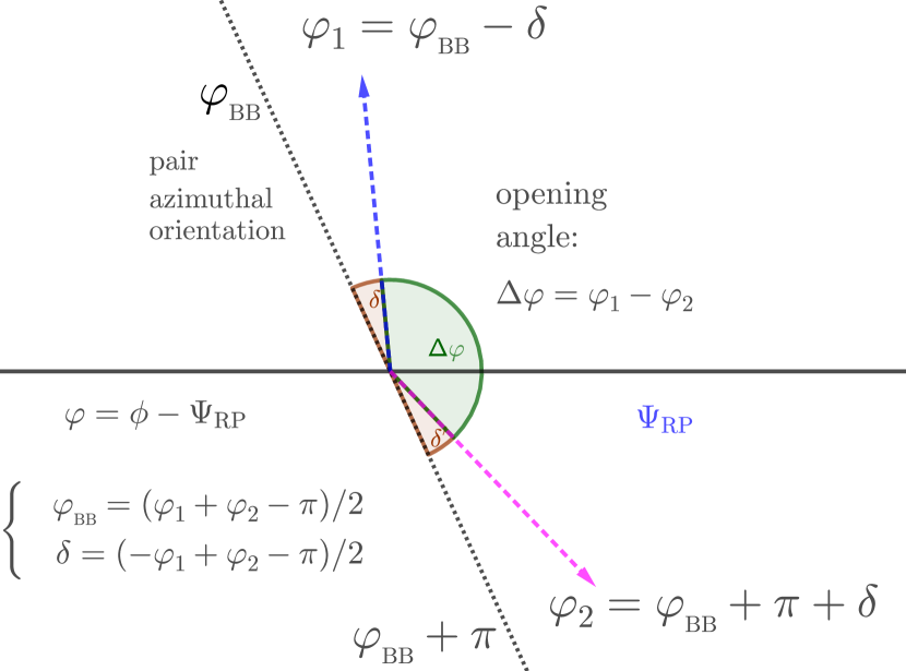
Figure 1: A sketch of “back-to-back” pair on the transverse plane.

We count the numbers of the OS (SS) pairs, $n_{\text{OS}}$ ($n_{\text{SS}}$), as a function of $\varphi_{\text{BB}}$. We define our new observable as

$$r_{\text{BB}}(\varphi_{\text{BB}})=\frac{n_{\text{OS}}(\varphi_{\text{BB}})-n_{\text{SS}}(\varphi_{\text{BB}})}{n_{\text{OS}}(\varphi_{\text{BB}})+n_{\text{SS}}(\varphi_{\text{BB}})}.$$ (2)

If we expand this ratio by Fourier series, as we will show in Sec. 2.2, the second-order coefficient of the Fourier expansion of this quantity is a measure of the CME signal.

2.2 CME signal extraction from $r_{\text{BB}}$

We first clarify analytically how $r_{\text{BB}}(\varphi_{\text{BB}})$ is sensitive to the CME signal. The azimuthal distribution for the primordial pions can be written as

$$n^{\pm}(\varphi)\equiv\frac{\text{d}N^{\pm}(\varphi)}{\text{d}\varphi}=\frac{N^{\pm}}{2\pi}(1\pm 2a_{1}\sin\varphi+2v_{2,\pi^{\pm}}\cos 2\varphi),$$ (3)

where the superscript $\pm$ means the charge sign, and $N^{\pm}$ is the total number of primordial $\pi^{\pm}$ of the event. The CME signal is described by the term $\pm 2a_{1}\sin\varphi$. A rough estimation is $\langle a_{1}^{2}\rangle\sim 10^{-4}$ in typical heavy ion collisions Kharzeev et al. (2008). Without loss of generality, we use $\varphi_{1}$ to denote a $\pi^{+}$ from the east subevent and $\varphi_{2}$ to denote a $\pi^{-}$ from the west subevent. Transferring to pair variables $\varphi_{\text{BB}}$ and $\delta$, noting the Jacob determinant $|\partial(\varphi_{1},\varphi_{2})/\partial(\varphi_{\text{BB}},\delta)|=2,$ we obtain the pair distribution

$$\begin{split}&n_{\text{W}}^{+}(\varphi_{1})n_{\text{E}}^{-}(\varphi_{2})\text{d}\varphi_{1}\text{d}\varphi_{2}\\ &=n_{\text{W}}^{+}(\varphi_{\text{BB}}-\delta)n_{\text{E}}^{-}(\varphi_{\text{BB}}+\pi+\delta)2\text{d}\varphi_{\text{BB}}\text{d}\delta.\end{split}$$ (4)

Including the other case, we have the OS pair density distribution

$$\begin{split}&n_{\text{OS}}(\varphi_{\text{BB}},\delta)\\ =&2n_{\text{W}}^{+}(\varphi_{\text{BB}}-\delta)n_{\text{E}}^{-}(\varphi_{\text{BB}}+\pi+\delta)\\ &+2n_{\text{W}}^{-}(\varphi_{\text{BB}}-\delta)n_{\text{E}}^{+}(\varphi_{\text{BB}}+\pi+\delta)\\ &=\frac{N_{\text{W}}^{+}N_{\text{E}}^{-}+N_{\text{W}}^{-}N_{\text{E}}^{+}}{2\pi^{2}}\Big{[}1+4a_{1}^{2}\sin(\varphi_{\text{BB}}+\delta)\sin(\varphi_{\text{BB}}-\delta)\\ &+4v_{2,\pi^{+}}v_{2,\pi^{-}}\cos 2(\varphi_{\text{BB}}+\delta)\cos 2(\varphi_{\text{BB}}-\delta)\\ &+\cos 2(\varphi_{\text{BB}}+\delta)\\ &\quad\times\left(v_{2,\pi^{+}}+v_{2,\pi^{-}}-2a_{1}(v_{2,\pi^{+}}-v_{2,\pi^{-}})\sin(\varphi_{\text{BB}}-\delta)\right)\\ &+\cos 2(\varphi_{\text{BB}}-\delta)\\ &\quad\times\left(v_{2,\pi^{+}}+v_{2,\pi^{-}}+2a_{1}(v_{2,\pi^{+}}-v_{2,\pi^{-}})\sin(\varphi_{\text{BB}}+\delta)\right)\Big{]}.\end{split}$$ (5)

Assuming the event averages

$$\langle N_{\text{W}}^{+}N_{\text{E}}^{-}\rangle=\langle N_{\text{W}}^{-}N_{\text{E}}^{+}\rangle=\langle N_{\text{W}}^{+}N_{\text{E}}^{+}\rangle=\langle N_{\text{W}}^{-}N_{\text{E}}^{-}\rangle=\langle N^{2}\rangle,$$ (6)

and intergrating over $\delta$ from $-\Delta$ to $\Delta$, we have

$$\begin{split}&n_{\text{OS}}(\varphi_{\text{BB}})=\int_{\delta=-\Delta}^{\delta=\Delta}n_{\text{OS}}(\varphi_{\text{BB}},\delta)\text{d}\delta\\ =&\frac{2\langle N^{2}\rangle}{\pi^{2}}\Big{[}\Delta+2v_{2,\pi^{+}}v_{2,\pi^{-}}\Delta\cos 4\varphi_{\text{BB}}+a_{1}^{2}\sin 2\Delta\\ &+\cos 2\varphi_{\text{BB}}(-2a_{1}^{2}\Delta+(v_{2,\pi^{+}}+v_{2,\pi^{-}})\sin 2\Delta)\\ &+\frac{1}{2}v_{2,\pi^{+}}v_{2,\pi^{-}}\sin 4\Delta\Big{]}.\end{split}$$ (7)

Similarly, we obtain the SS pair density distribution

$$\begin{split}&n_{\text{SS}}(\varphi_{\text{BB}},\delta)\\ =&2n_{\text{W}}^{+}(\varphi_{\text{BB}}-\delta)n_{\text{E}}^{+}(\varphi_{\text{BB}}+\pi+\delta)\\ &+2n_{\text{W}}^{-}(\varphi_{\text{BB}}-\delta)n_{\text{E}}^{-}(\varphi_{\text{BB}}+\pi+\delta),\end{split}$$ (8)

$$\begin{split}&n_{\text{SS}}(\varphi_{\text{BB}})=\int_{\delta=-\Delta}^{\delta=\Delta}n_{\text{SS}}(\varphi_{\text{BB}},\delta)\text{d}\delta\\ =&\frac{2\langle N^{2}\rangle}{\pi^{2}}\Big{[}\Delta+(v_{2,\pi^{+}}^{2}+v_{2,\pi^{-}}^{2})\Delta\cos 4\varphi_{\text{BB}}-a_{1}^{2}\sin 2\Delta\\ &+\cos 2\varphi_{\text{BB}}(2a_{1}^{2}\Delta+(v_{2,\pi^{+}}+v_{2,\pi^{-}})\sin 2\Delta)\\ &+\frac{1}{4}(v_{2,\pi^{+}}^{2}+v_{2,\pi^{-}}^{2})\sin 4\Delta\Big{]}.\end{split}$$ (9)

The difference and sum are, respectively,

$$\begin{split}&n_{\text{OS}}(\varphi_{\text{BB}})-n_{\text{SS}}(\varphi_{\text{BB}})\\ =&\frac{2\langle N^{2}\rangle}{\pi^{2}}\Big{[}-4a_{1}^{2}\Delta\cos 2\varphi_{\text{BB}}+2a_{1}^{2}\sin 2\Delta\\ &-(v_{2,\pi^{+}}-v_{2,\pi^{-}})^{2}\Delta\cos 4\varphi_{\text{BB}}\\ &-\frac{1}{4}(v_{2,\pi^{+}}-v_{2,\pi^{-}})^{2}\sin 4\Delta\Big{]},\end{split}$$ (10)

$$\begin{split}&n_{\text{OS}}(\varphi_{\text{BB}})+n_{\text{SS}}(\varphi_{\text{BB}})\\ =&\frac{2\langle N^{2}\rangle}{\pi^{2}}\Big{[}2\Delta+(v_{2,\pi^{+}}+v_{2,\pi^{-}})^{2}\Delta\cos 4\varphi_{\text{BB}}\\ &+(v_{2,\pi^{+}}+v_{2,\pi^{-}})\cos 2\varphi_{\text{BB}}\sin 2\Delta\\ &+\frac{1}{4}(v_{2,\pi^{+}}+v_{2,\pi^{-}})^{2}\sin 4\Delta\Big{]}.\end{split}$$ (11)

Our new observable is the ratio and we expand it into Fourier series

$$r_{\text{BB}}(\varphi_{\text{BB}})=\frac{n_{\text{OS}}(\varphi_{\text{BB}})-n_{\text{SS}}(\varphi_{\text{BB}})}{n_{\text{OS}}(\varphi_{\text{BB}})+n_{\text{SS}}(\varphi_{\text{BB}})}=\sum_{k=0}^{+\infty}c_{k}\cos(k\varphi_{\text{BB}}).$$ (12)

Noticing that $(v_{2,\pi^{+}}+v_{2,\pi^{-}})$ is small ($\sim 0.1$), up to the first order of $(v_{2,\pi^{+}}+v_{2,\pi^{-}})$, the coefficient of $\cos 2\varphi_{\text{BB}}$ is

$$\begin{split}&c_{2}\approx a_{1}^{2}\left(-2-(v_{2,\pi^{+}}+v_{2,\pi^{-}})\frac{\sin^{2}2\Delta}{\Delta^{2}}\right)\\ &+(v_{2,\pi^{+}}+v_{2,\pi^{-}})(v_{2,\pi^{+}}-v_{2,\pi^{-}})^{2}\frac{(2\Delta+\sin 4\Delta)\sin 2\Delta}{8\Delta^{2}}.\end{split}$$ (13)

If we require the opening angle to be larger than $150^{\circ}$ for the back-to-back pairs, then $\Delta=15^{\circ}$,

$$\begin{split}c_{2}\approx&a_{1}^{2}\left(-2-3.648(v_{2,\pi^{+}}+v_{2,\pi^{-}})\right)\\ &+1.267(v_{2,\pi^{+}}+v_{2,\pi^{-}})(v_{2,\pi^{+}}-v_{2,\pi^{-}})^{2}.\end{split}$$ (14)

The second term is not related to the CME; taking $|v_{2,\pi^{+}}-v_{2,\pi^{-}}|\sim 10^{-3},\quad(v_{2,\pi^{+}}+v_{2,\pi^{-}})\sim 10^{-1}$, its magnitude is on the order of $10^{-7}$. For a CME signal of $a_{1}\geq 10^{-3}$, $a_{1}^{2}$ dominates over the primordial flow effects in $c_{2}$, indicating that $c_{2}$ is a good measure of the CME.

Similarly, the coefficient of the constant term ($k=0$) is

$$\begin{split}c_{0}=&\frac{\sin 2\Delta}{4\Delta}\big{(}4a_{1}^{2}(1+v_{2,\pi^{+}}+v_{2,\pi^{-}})\\ &-(v_{2,\pi^{+}}-v_{2,\pi^{-}})^{2}\cos 2\Delta\big{)},\end{split}$$ (15)

and for $\Delta=15^{\circ}$,

$$\begin{split}c_{0}\approx 1.910a_{1}^{2}(1+v_{2,\pi^{+}}+v_{2,\pi^{-}})-1.654(v_{2,\pi^{+}}-v_{2,\pi^{-}})^{2}.\end{split}$$ (16)

Note that $c_{2}$ and $c_{0}$ are both sensitive to the CME, with similar sensitivities. It will be shown later, however, that $c_{0}$ is also sensitive to the backgrounds. Those backgrounds are mainly from the low $p_{T}$ resonance decays whose decay daughters are back-to-back. The $c_{2}$ is less sensitive to those backgrounds because their $v_{2}$ at low $p_{T}$ is small.

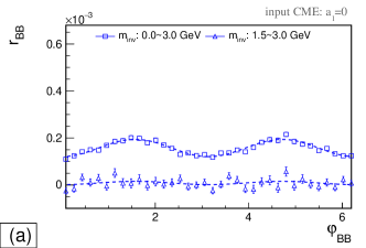
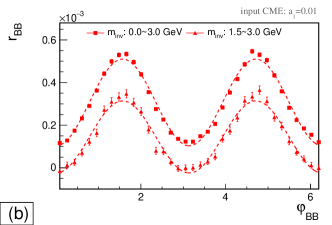
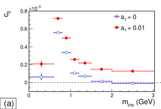
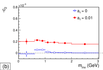
Figure 2: The distribution of the back-to-back relative-excess observable $r_{\text{BB}}(\varphi_{\text{BB}})$ in the toy model simulations with input CME (a) $a_{1}=0$ and (b) $a_{1}=0.01$.

Figure 3: The fitted Fourier coefficients, (a) $c_{0}$ and (b) $-c_{2}$, to the back-to-back relative-excess observable $r_{\text{BB}}(\varphi_{\text{BB}})$ in the toy model with various CME inputs.

2.3 Comparison to the back-to-back $\Delta\gamma$ observable, $\Delta\gamma_{\text{BB}}$

The $\Delta\gamma$ observable is frequently used in heavy-ion collisions to search for the CME,

$$\begin{split}\Delta\gamma=&\gamma_{\text{OS}}-\gamma_{\text{SS}},\\ \gamma=&\langle\cos(\varphi_{1}+\varphi_{2})\rangle.\end{split}$$ (17)

To see the relationship between $r_{\text{BB}}$ and $\Delta\gamma$, we will apply the same “back-to-back” requirement to the pairs in $\Delta\gamma$, denoted as $\Delta\gamma_{\text{BB}}$. For back-to-back pairs, $\cos(\varphi_{1}+\varphi_{2})=-\cos(2\varphi_{\text{BB}})$. The correlators $\gamma_{\text{OS}}$ and $\gamma_{\text{SS}}$ can be simplified into

$$\begin{split}\gamma_{\text{OS}}=&-\frac{\int\cos(2\varphi_{\text{BB}})n_{\text{OS}}(\varphi_{\text{BB}})\text{d}\varphi_{\text{BB}}}{\int n_{\text{OS}}(\varphi_{\text{BB}})\text{d}\varphi_{\text{BB}}}\\ =&\frac{2a_{1}^{2}\Delta-(v_{2,\pi^{+}}+v_{2,\pi^{-}})\sin 2\Delta}{2\Delta+2a_{1}^{2}\sin 2\Delta+v_{2,\pi^{-}}v_{2,\pi^{+}}\sin 4\Delta},\\ \gamma_{\text{SS}}=&-\frac{\int\cos(2\varphi_{\text{BB}})n_{\text{SS}}(\varphi_{\text{BB}})\text{d}\varphi_{\text{BB}}}{\int n_{\text{SS}}(\varphi_{\text{BB}})\text{d}\varphi_{\text{BB}}}\\ =&\frac{-2a_{1}^{2}\Delta-(v_{2,\pi^{+}}+v_{2,\pi^{-}})\sin 2\Delta}{2\Delta-2a_{1}^{2}\sin 2\Delta+\frac{1}{2}(v_{2,\pi^{-}}^{2}+v_{2,\pi^{+}}^{2})\sin 4\Delta}.\end{split}$$ (18)

The difference to the first order of $(v_{2,\pi^{+}}+v_{2,\pi^{-}})$ is therefore

$$\begin{split}\Delta\gamma_{\text{BB}}=&\gamma_{\text{OS}}-\gamma_{\text{SS}}\\ \approx&a_{1}^{2}\left(2+(v_{2,\pi^{+}}+v_{2,\pi^{-}})\frac{\sin^{2}2\Delta}{\Delta^{2}}\right)\\ &-(v_{2,\pi^{+}}+v_{2,\pi^{-}})(v_{2,\pi^{+}}-v_{2,\pi^{-}})^{2}\frac{\sin 2\Delta\sin 4\Delta}{8\Delta^{2}}.\end{split}$$ (19)

With $\Delta=15^{\circ}$, it becomes

$$\begin{split}\Delta\gamma_{\text{BB}}=&\gamma_{\text{OS}}-\gamma_{\text{SS}}\\ \approx&a_{1}^{2}\left(2+3.648(v_{2,\pi^{+}}+v_{2,\pi^{-}})\right)\\ &-0.790(v_{2,\pi^{+}}+v_{2,\pi^{-}})(v_{2,\pi^{+}}-v_{2,\pi^{-}})^{2}.\end{split}$$ (20)

Comparing Eqs. 19 and 20 to Eqs. 13 and 14, it is clear that $\Delta\gamma_{\text{BB}}$ and $r_{\text{BB}}$ have similar sensitivity to the CME. The $r_{\text{BB}}$ observable is directly related to $\Delta\gamma_{\text{BB}}$. Only the back-to-back pairs are used in these two observables, so the backgrounds among the close pairs are reduced.

3 Results

In this section, we show the back-to-back $r_{\text{BB}}(\varphi_{\text{BB}})$ and back-to-back $\Delta\gamma_{\text{BB}}$ observables calculated from a toy model (with/without input CME) simulations.

3.1 Toy-model simulation

We use a toy model including the primordial pions and the $\rho$ meson decays to study the sensitivities of $r_{\text{BB}}$ to CME signal and resonance backgrounds. This toy model has been used for CME background studies in Ref. Wang and Zhao (2017); Feng et al. (2018). Both the resonance decays and primordial pions have the $p_{T}$ distributions and $v_{2}(p_{T})$ obtained from Au+Au measurements corresponding to centrality $40\%\sim 50\%$ Adams et al. (2004a); Adler et al. (2003); Adams et al. (2004b); Abelev et al. (2009b); Adams et al. (2005); Adare et al. (2010); Dong et al. (2004); Adamczyk et al. (2015); Olive et al. (2014); Abelev et al. (2010b); Wang and Zhao (2017).

To simulate the CME signal in the toy model, we input the coefficient $a_{1}$ when generating the primordial pions from the azimuthal distribution (Eq. 3). Two cases are studied, one without CME input ($a_{1}=0$), and the other with $1\%$ CME input ($a_{1}=0.01$). Each case has $2\times 10^{9}$ events. The tracks are selected with transverse momentum $0.2\text{ GeV}<p_{T}<2.0\text{ GeV}$ and pseudorapidity $-1.0<\eta<1.0$. Figure 3 shows the $r_{\text{BB}}(\varphi_{\text{BB}})$ distributions for the two cases. The case with finite CME shows larger amplitude and modulation than the case without, indicating the sensitivity of the $r_{\text{BB}}(\varphi_{\text{BB}})$ observable to the CME. The case without CME shows some finite amplitude and modulation, at low $m_{\text{inv}}$, indicating that the observable still has some background contamination. In order to further suppress resonance backgrounds, we also show the $r_{\text{BB}}$ distributions with the invariant mass range $1.5\text{ GeV}<m_{\text{inv}}<3.0\text{ GeV}$. The result is consistent with zero as expected.

$m_{\text{inv}}$ range (GeV)	input $a_{1}$	Fourier coefficients ($\times 10^{-4}$)		extracted $a_{1}$ ($\times 10^{-2}$)
$0.0\sim 3.0$	$0$	$\ \ c_{0}$	$1.57\pm 0.01$	$0.87\pm 0.01$
		$-c_{2}$	$0.37\pm 0.02$	$0.39\pm 0.02$
	$0.01$	$\ \ c_{0}$	$3.07\pm 0.01$	$1.21\pm 0.01$
		$-c_{2}$	$2.04\pm 0.02$	$0.93\pm 0.01$
$1.5\sim 3.0$	$0$	$\ \ c_{0}$	$0.08\pm 0.03$	$0.20\pm 0.07$
		$-c_{2}$	$0.07\pm 0.04$	$0.17\pm 0.10$
	$0.01$	$\ \ c_{0}$	$1.45\pm 0.03$	$0.83\pm 0.02$
		$-c_{2}$	$1.69\pm 0.04$	$0.85\pm 0.02$

Table 1: The fitted Fourier coefficients $c_{0}$ and $-c_{2}$ are shown for the $r_{\text{BB}}(\varphi_{\text{BB}})$ distributions from the toy-model simulations with/without CME signal input. Two invariant mass ranges are shown. If we set $(v_{2,\pi^{+}}+v_{2,\pi^{-}})\approx 0.1$, ignore the $(v_{2,\pi^{+}}-v_{2,\pi^{-}})^{2}$ terms in Eqs. 14 and 16, and assume zero resonance background in the toy-model simulations, the $a_{1}$ can be extracted from $c_{0}$ and $c_{2}$, respectively. These extracted $a_{1}$ values are also listed, to be compared to the input $a_{1}$.

We fit the $r_{\text{BB}}(\varphi_{\text{BB}})$ distributions to Eq. 12. Figure 3 shows the fitted Fourier coefficients $c_{0}$ and $-c_{2}$, respectively, as a function of $m_{\text{inv}}$. The $c_{0}$ has strong sensitivity to both signal and background. Although still affected by the residual resonance backgrounds, the $-c_{2}$ has better sensitivity to CME than $c_{0}$ and less sensitivity to background. To illustrate our results more quantitatively, we list the fitted coefficients $c_{0}$ and $-c_{2}$ in Table 1. Also listed are the $a_{1}$ values extracted from $c_{0}$ and $-c_{2}$, via Eqs. 16 and 14, respectively, ignoring the presence of backgrounds. Due to resonance backgrounds in the low $m_{\text{inv}}$ range, the extracted $a_{1}$ are large with $0.0\text{ GeV}<m_{\text{inv}}<3.0\text{ GeV}$, no matter whether the input $a_{1}$ are zero or not. In the range $1.5\text{ GeV}<m_{\text{inv}}<3.0\text{ GeV}$, with zero input $a_{1}$, the extracted $a_{1}$ values are also close to zero; the small deviations from zero are due to residual resonance backgrounds. With input $a_{1}=0.01$, the extracted $a_{1}$ values in the high $m_{\text{inv}}$ range are nonzero, close to the input; again, the differences are due to residual resonance backgrounds. However, under this condition, the extracted $a_{1}$ values are smaller than the inputs. This is because there are pairs composed of pions from uncorrelated sources (one primordial pion and one resonance pion, or two pions from two different resonance decays), whose zero contributions are averaged in $c_{0}$, $-c_{2}$. The dilution from those uncorrelated pairs reduces the extracted $a_{1}$ values.

3.2 Comparison among $\Delta\gamma$, $\Delta\gamma_{\text{BB}}$, and $-c_{2}$

We also calculate the inclusive $\Delta\gamma$ and back-to-back $\Delta\gamma_{\text{BB}}$ observables in our model studies. Figure 4 compares the results of those three observables. It is found that $\Delta\gamma_{\text{BB}}$ and $-c_{2}$ are very close to each other. This indicates that the $r_{\text{BB}}$ and $\Delta\gamma_{\text{BB}}$ observables are nearly the same, as expected from Eqs. 14 and 20. With zero CME input ($a_{1}=0$) in the toy model simulation (Fig. 4a), the inclusive $\Delta\gamma$ is further away from zero than the other two observables in the invariant mass range $0.6\sim 1.5\text{ GeV}$ where resonance contributions are large. This shows that the inclusive $\Delta\gamma$ is more significantly affected by the resonance backgrounds. In the high mass region where resonance contributions are small, all three observables approach to zero as expected. With nonzero CME input ($a_{1}=0.01$) in the toy model simulation (Fig. 4b), the three observables are all away from zero. The inclusive $\Delta\gamma$ is lower than the other two in the mass range $1.5\text{ GeV}\sim 3.0\text{ GeV}$ where there is not much resonance contribution. This is because the back-to-back CME signal is diluted more in the inclusive $\Delta\gamma$ by including close pairs from backgrounds. This can also be explained by the analytical calculations in Eq. 19 by assigning $\Delta=90^{\circ}$ for the inclusive $\Delta\gamma$ and $\Delta=15^{\circ}$ for $\Delta\gamma_{\text{BB}}$.

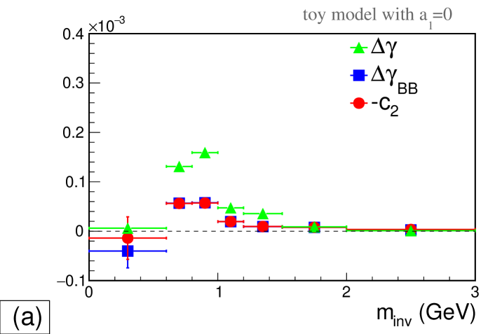
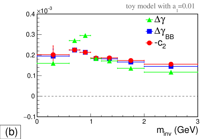
Figure 4: Comparison among the inclusive $\Delta\gamma$, the back-to-back $\Delta\gamma_{\text{BB}}$, and the Fourier coefficient $-c_{2}$ of the $r_{\text{BB}}(\varphi_{\text{BB}})$ distribution in different simulations.

4 Summary

In this paper, we propose a new observable to search for the CME, called the back-to-back relative-excess observable of OS to SS pairs ($r_{\text{BB}}$), as a function of the pair azimuthal orientation ($\varphi_{\text{BB}}$). The charge pairs used in this observable are required to be back-to-back: opening angle larger than $150^{\circ}$ on the transverse plane; they are taken from different $\eta$ ranges with a $\Delta\eta$ gap to further reduce backgrounds. As a result, the backgrounds (such as resonance decays) contributing mostly to the close pairs can be reduced. A modulation of the form $\cos 2\varphi_{\text{BB}}$ in the observable can indicate a CME signal, which is described by the second-order coefficient $c_{2}$ in Fourier expansion.

We use a toy model simulation without input CME ($a_{1}=0$) and with $1\%$ input CME ($a=0.01$), and calculate the observable from the simulated data. The coefficient $c_{2}$ is close to zero when there is no input CME, whereas it is far from zero with $1\%$ input CME.

To relate the new observable to the previous $\Delta\gamma$ observable, we apply the same back-to-back pair requirement to the definition of $\Delta\gamma$ to obtain $\Delta\gamma_{\text{BB}}$. We use analytical calculations and toy-model simulations to show that $\Delta\gamma_{\text{BB}}$ is nearly identical to $-c_{2}$. Both are more sensitive to the CME and less sensitive to resonance backgrounds than the inclusive $\Delta\gamma$ observable.

References

- Lee and Wick (1974) T. Lee and G. Wick, Vacuum stability and vacuum excitation in a spin 0 field theory, Phys.Rev. D9, 2291 (1974).
- Morley and Schmidt (1985) P. D. Morley and I. A. Schmidt, Strong P, CP, T violations in heavy ion collisions, Z. Phys. C26, 627 (1985).
- Kharzeev et al. (1998) D. Kharzeev, R. Pisarski, and M. H. Tytgat, Possibility of spontaneous parity violation in hot QCD, Phys.Rev.Lett. 81, 512 (1998), arXiv:hep-ph/9804221 [hep-ph] .
- Kharzeev et al. (2008) D. E. Kharzeev, L. D. McLerran, and H. J. Warringa, The Effects of topological charge change in heavy ion collisions: ’Event by event P and CP violation’, Nucl.Phys. A803, 227 (2008), arXiv:0711.0950 [hep-ph] .
- Abelev et al. (2009a) B. Abelev et al. (STAR Collaboration), Azimuthal Charged-Particle Correlations and Possible Local Strong Parity Violation, Phys.Rev.Lett. 103, 251601 (2009a), arXiv:0909.1739 [nucl-ex] .
- Abelev et al. (2010a) B. Abelev et al. (STAR Collaboration), Observation of charge-dependent azimuthal correlations and possible local strong parity violation in heavy ion collisions, Phys.Rev. C81, 054908 (2010a), arXiv:0909.1717 [nucl-ex] .
- Adamczyk et al. (2014a) L. Adamczyk et al. (STAR), Beam-energy dependence of charge separation along the magnetic field in Au+Au collisions at RHIC, Phys. Rev. Lett. 113, 052302 (2014a), arXiv:1404.1433 [nucl-ex] .
- Adamczyk et al. (2013) L. Adamczyk et al. (STAR), Fluctuations of charge separation perpendicular to the event plane and local parity violation in GeV Au+Au collisions at the BNL Relativistic Heavy Ion Collider, Phys. Rev. C88, 064911 (2013), arXiv:1302.3802 [nucl-ex] .
- Zhao (2018a) J. Zhao (STAR), Chiral magnetic effect search in p+Au, d+Au and Au+Au collisions at RHIC, Proceedings, 47th International Symposium on Multiparticle Dynamics (ISMD2017): Tlaxcala, Tlaxcala, Mexico, September 11-15, 2017, EPJ Web Conf. 172, 01005 (2018a), arXiv:1712.00394 [hep-ex] .
- Zhao (2017) J. Zhao (STAR), Charge dependent particle correlations motivated by chiral magnetic effect and chiral vortical effect, Proceedings, 46th International Symposium on Multiparticle Dynamics (ISMD 2016): Jeju Island, South Korea, August 29-September 2, 2016, EPJ Web Conf. 141, 01010 (2017).
- Zhao (2019) J. Zhao, Measurements of the chiral magnetic effect with background isolation in 200 gev au+au collisions at star, Nuclear Physics A 982, 535 (2019), the 27th International Conference on Ultrarelativistic Nucleus-Nucleus Collisions: Quark Matter 2018.
- Adamczyk et al. (2014b) L. Adamczyk et al. (STAR), Measurement of charge multiplicity asymmetry correlations in high-energy nucleus-nucleus collisions at 200 GeV, Phys. Rev. C89, 044908 (2014b), arXiv:1303.0901 [nucl-ex] .
- Khachatryan et al. (2017) V. Khachatryan et al. (CMS), Observation of charge-dependent azimuthal correlations in -Pb collisions and its implication for the search for the chiral magnetic effect, Phys. Rev. Lett. 118, 122301 (2017), arXiv:1610.00263 [nucl-ex] .
- Abelev et al. (2013) B. Abelev et al. (ALICE), Charge separation relative to the reaction plane in Pb-Pb collisions at TeV, Phys.Rev.Lett. 110, 012301 (2013), arXiv:1207.0900 [nucl-ex] .
- Acharya et al. (2018) S. Acharya et al. (ALICE), Constraining the magnitude of the Chiral Magnetic Effect with Event Shape Engineering in Pb-Pb collisions at = 2.76 TeV, Phys. Lett. B777, 151 (2018), arXiv:1709.04723 [nucl-ex] .
- Sirunyan et al. (2018) A. M. Sirunyan et al. (CMS Collaboration), Constraints on the chiral magnetic effect using charge-dependent azimuthal correlations in p-pb and pb-pb collisions at the cern large hadron collider, Phys. Rev. C 97, 044912 (2018).
- Voloshin (2004) S. A. Voloshin, Parity violation in hot QCD: How to detect it, Phys.Rev. C70, 057901 (2004), arXiv:hep-ph/0406311 [hep-ph] .
- Wang (2010) F. Wang, Effects of Cluster Particle Correlations on Local Parity Violation Observables, Phys.Rev. C81, 064902 (2010), arXiv:0911.1482 [nucl-ex] .
- Bzdak et al. (2010) A. Bzdak, V. Koch, and J. Liao, Remarks on possible local parity violation in heavy ion collisions, Phys.Rev. C81, 031901 (2010), arXiv:0912.5050 [nucl-th] .
- Schlichting and Pratt (2011) S. Schlichting and S. Pratt, Charge conservation at energies available at the BNL Relativistic Heavy Ion Collider and contributions to local parity violation observables, Phys.Rev. C83, 014913 (2011), arXiv:1009.4283 [nucl-th] .
- Xu et al. (2018a) H.-j. Xu, X. Wang, H. Li, J. Zhao, Z.-W. Lin, C. Shen, and F. Wang, Importance of isobar density distributions on the chiral magnetic effect search, Phys. Rev. Lett. 121, 022301 (2018a).
- Xu et al. (2018b) H.-J. Xu, J. Zhao, X.-B. Wang, H.-L. Li, Z.-W. Lin, C.-W. Shen, and F.-Q. Wang, Varying the chiral magnetic effect relative to flow in a single nucleus-nucleus collision, Chinese Physics C 42, 084103 (2018b).
- Liao et al. (2010) J. Liao, V. Koch, and A. Bzdak, On the Charge Separation Effect in Relativistic Heavy Ion Collisions, Phys.Rev. C82, 054902 (2010), arXiv:1005.5380 [nucl-th] .
- Bzdak et al. (2011) A. Bzdak, V. Koch, and J. Liao, Azimuthal correlations from transverse momentum conservation and possible local parity violation, Phys.Rev. C83, 014905 (2011), arXiv:1008.4919 [nucl-th] .
- Pratt et al. (2011) S. Pratt, S. Schlichting, and S. Gavin, Effects of Momentum Conservation and Flow on Angular Correlations at RHIC, Phys.Rev. C84, 024909 (2011), arXiv:1011.6053 [nucl-th] .
- Petersen et al. (2011) H. Petersen, T. Renk, and S. A. Bass, Medium-modified Jets and Initial State Fluctuations as Sources of Charge Correlations Measured at RHIC, Phys.Rev. C83, 014916 (2011), arXiv:1008.3846 [nucl-th] .
- Toneev et al. (2012) V. Toneev, V. Konchakovski, V. Voronyuk, E. Bratkovskaya, and W. Cassing, Event-by-event background in estimates of the chiral magnetic effect, Phys.Rev. C86, 064907 (2012), arXiv:1208.2519 [nucl-th] .
- Zhao (2018b) J. Zhao, Search for the Chiral Magnetic Effect in Relativistic Heavy-Ion Collisions, Int. J. Mod. Phys. A33, 1830010 (2018b), arXiv:1805.02814 [nucl-ex] .
- Jie Zhao (2018) F. W. Jie Zhao, Zhoudunming Tu, Status of the chiral magnetic effect search in relativistic heavy-ion collisions, Nuclear Physics Review 35, 225 (2018), arXiv:1807.05083 [nucl-ex] .
- Zhao and Wang (2019) J. Zhao and F. Wang, Experimental searches for the chiral magnetic effect in heavy-ion collisions, Prog. Part. Nucl. Phys. 107, 200 (2019), arXiv:1906.11413 [nucl-ex] .
- Wang and Zhao (2017) F. Wang and J. Zhao, Challenges in flow background removal in search for the chiral magnetic effect, Phys. Rev. C95, 051901 (2017), arXiv:1608.06610 [nucl-th] .
- Feng et al. (2018) Y. Feng, J. Zhao, and F. Wang, Responses of the chiral-magnetic-effect–sensitive sine observable to resonance backgrounds in heavy-ion collisions, Phys. Rev. C 98, 034904 (2018), arXiv:1803.02860 [nucl-th] .
- Adams et al. (2004a) J. Adams et al. (STAR), Rho0 production and possible modification in Au+Au and p+p collisions at S(NN)**1/2 = 200-GeV, Phys. Rev. Lett. 92, 092301 (2004a), arXiv:nucl-ex/0307023 [nucl-ex] .
- Adler et al. (2003) S. Adler et al. (PHENIX Collaboration), Suppressed production at large transverse momentum in central Au+ Au collisions at S(NN)**1/2 = 200 GeV, Phys.Rev.Lett. 91, 072301 (2003), arXiv:nucl-ex/0304022 [nucl-ex] .
- Adams et al. (2004b) J. Adams et al. (STAR), Identified particle distributions in pp and Au+Au collisions at s(NN)**(1/2) = 200 GeV, Phys. Rev. Lett. 92, 112301 (2004b), arXiv:nucl-ex/0310004 [nucl-ex] .
- Abelev et al. (2009b) B. Abelev et al. (STAR Collaboration), Systematic measurements of identified particle spectra in , +Au and Au+Au collisions from STAR, Phys.Rev. C79, 034909 (2009b), arXiv:0808.2041 [nucl-ex] .
- Adams et al. (2005) J. Adams et al. (STAR Collaboration), Azimuthal anisotropy in Au+Au collisions at s(NN)**(1/2) = 200-GeV, Phys.Rev. C72, 014904 (2005), arXiv:nucl-ex/0409033 [nucl-ex] .
- Adare et al. (2010) A. Adare et al. (PHENIX), Azimuthal anisotropy of neutral pion production in Au+Au collisions at = 200 GeV: Path-length dependence of jet quenching and the role of initial geometry, Phys. Rev. Lett. 105, 142301 (2010), arXiv:1006.3740 [nucl-ex] .
- Dong et al. (2004) X. Dong, S. Esumi, P. Sorensen, N. Xu, and Z. Xu, Resonance decay effects on anisotropy parameters, Phys. Lett. B597, 328 (2004), arXiv:nucl-th/0403030 [nucl-th] .
- Adamczyk et al. (2015) L. Adamczyk et al. (STAR), Measurements of Dielectron Production in AuAu Collisions at = 200 GeV from the STAR Experiment, Phys. Rev. C92, 024912 (2015), arXiv:1504.01317 [hep-ex] .
- Olive et al. (2014) K. A. Olive et al. (Particle Data Group), Review of Particle Physics, Chin. Phys. C38, 090001 (2014).
- Abelev et al. (2010b) B. Abelev et al. (STAR Collaboration), Studying Parton Energy Loss in Heavy-Ion Collisions via Direct-Photon and Charged-Particle Azimuthal Correlations, Phys.Rev. C82, 034909 (2010b), arXiv:0912.1871 [nucl-ex] .