A linearly implicit energy-preserving exponential integrator for the nonlinear Klein-Gordon equation

Abstract

In this paper, we generalize the exponential energy-preserving integrator proposed in the recent paper [SIAM J. Sci. Comput. 38(2016) A1876-A1895] for conservative systems, which now becomes linearly implicit by further utilizing the idea of the scalar auxiliary variable approach. Comparing with the original exponential energy-preserving integrator which usually leads to a nonlinear algebraic system, our new method only involve a linear system with constant coefficient matrix. Taking the nonlinear Klein-Gordon equation for example, we derive the concrete energy-preserving scheme and demonstrate its high efficiency through numerical experiments.

AMS subject classification: 65L05, 65M06, 65M20, 65M70
Keywords: Scalar auxiliary variable approach, linearly implicit scheme, energy-preserving scheme, conservative system.

1 Introduction

It is well-known that exponential integrators permit larger step sizes and achieve higher accuracy than nonexponential ones when the considered problem is a very stiff differential equation such as highly oscillatory ODEs or semidiscrete time-dependent PDEs. As to exponential integrators, the earlier attempts can date back to the original paper by Hersch [20], whereas the term “exponential integrators” was coined in the seminal paper by Hochbruck, Lubich, and Selhofer [22]. Readers are referred to Ref. [23] for details about exponential integrators. Over the years, there has been growing interest in structure-preserving exponential methods, which can preserve as much as possible the physical/geromeric properties of the dynamic system under consideration [18]. Due to the superior properties in the capability for the long-term computation, symplectic exponential methods have attracted much attention (e.g., see Refs. [33, 39, 45] and references therein). On the other hand, the energy conservation law is an important property of conservative systems and whether or not can preserve the energy conservation law of the original systems is a criterion to judge the success of a numerical method for their solution (e.g. see Refs. [14, 29, 47] and references therein). Thus, how to design energy-preserving schemes for conservative systems attracts a lot of interest in recent years. The noticeable ones include the discrete gradient (including averaged vector filed (AVF) method) [5, 7, 28, 35, 32], discrete variational derivative method [10, 14], Hamiltonian Boundary Value Methods (HBVMs) [2], energy-preserving continuous stage Runge-Kutta (CSRK) methods [17, 34, 42] and local energy-preserving methods [3, 15, 25, 44], and so on. However, to our best knowledge, most existing works on exponential integrators up to now focus on the construction of explicit schemes and fail to be energy-preserving. In Ref. [6], Celledoni et al. proposed some implicit and exponential integrators that preserver symmetric and energy of the cubic Schrödinger equation by using the symmetric projection approach [18]. Recently, combining the ideas of exponential integrators and discrete gradients, Li and Wu [30] proposed an energy-preserving exponential scheme for conservative systems, which was revisited and generalized more recently by Shen and Leok [39]. Unfortunately, such scheme is fully implicit. At each time step, one needs to solve a fully nonlinear system and thus it might be very time consuming. Compared with fully implicit schemes, linearly implicit schemes only require to solve a linear system, which leads to considerably lower costs than implicit ones [10]. As far as we know, there has been no reference considering linearly implicit exponential schemes for conservative systems, which can inherit the energy.

In this paper, taking the nonlinear Klein-Gordon equation as an example, we propose a novel linearly implicit exponential scheme for conservative systems by combining the ideas of the exponential integrator and the scalar auxiliary variable (SAV) approach [37, 38]. The proposed scheme can inherit the energy and enjoy the same computational advantages as the one (see [4]) provided by the classical SAV approach. The SAV approach as well as the earlier invariant energy quadratization (IEQ) approach [46, 48] is developed based on the idea of the energy quadratization, which can result linearly implicit and energy stable schemes for gradient flows. To the best of our knowledge, there has been no reference considering the combination of the ideas of the SAV approach and the exponential integrator for developing linearly implicit energy-preserving schemes for energy-conserving systems. Taking the nonlinear Klein-Gordon equation for example, we first explore the feasibility.

The outline of this paper is organized as follows. In Section 2, based on idea of the SAV approach, the NKGE (2.1) is reformulated into an equivalent system which inherits a modified energy. In Section 3, a second-order centered difference method is applied to the system and we show that the resulting semi-discrete system can preserve the semi-discrete energy. In Section 4, a linearly implicit exponential scheme is presented by combining the exponential integrator and the linearized Crank-Nicolson method, which inherits the fully discrete energy. Several numerical examples are shown to illustrate the power of our proposed scheme in Section 5. We draw some conclusions in Section 6.

2 Reformation of the model equation through the SAV approach

The Klein-Gordon equation is frequently used in mathematical models for problems in many fields of science and engineering, particularly in quantum field theory and relativistic quantum mechanics. Here, we consider the following nonlinear Klein-Gordon equation (NKGE)

$$\left\{\begin{aligned} &\partial_{tt}u({\bm{x}},t)-\omega^{2}\Delta u({\bm{x}},t)+G^{{}^{\prime}}(u({\bm{x}},t))=0,\ {\bm{x}}\in\mathbb{R}^{d},\ t>0,\\ &u({\bm{x}},0)=\phi_{1}({\bm{x}}),\ \partial_{t}u({\bm{x}},0)=\phi_{2}({\bm{x}}),\ {\bm{x}}\in\mathbb{R}^{d},\end{aligned}\right.$$ (2.1)

where $t$ is time variable, ${\bm{x}}\in\mathbb{R}^{d}$ is the spatial variable, $u:=u({\bm{x}},t)$ is a real-valued function, $\omega$ is a real parameter, $\Delta$ is the usual Laplace operator, $G(u)$ is a smooth potential energy function with $G(u)\geq 0$, and $\phi_{1}:=\phi_{1}({\bm{x}})$ and $\phi_{2}:=\phi_{2}({\bm{x}})$ are two given real-value initial data. The NKGE (2.1) conserves the Hamiltonian energy

$$E(t) =\int_{\mathbb{R}^{d}}\Big{[}\frac{1}{2}|\partial_{t}u|^{2}+\frac{\omega^{2}}{2}|\nabla u|^{2}+G(u)\Big{]}d{\bm{x}}=E(0),\ t\geq 0.$$ (2.2)

In the last few decades, various structure-preserving methods have been developed for solving the NKGE (2.1), including symplectic methods ( e.g., see Refs. [13, 31, 33]), multisymplectic methods (e.g., see Refs. [24, 36, 41, 49]) and energy-preserving methods (e.g., see Refs. [1, 9, 16, 43]), etc. However, there has been no reference considering a linearly implicit structure-preserving exponential scheme for the NKGE (2.1) to our knowledge.

Following the idea of the SAV approach, we introduce a scalar auxiliary variable, as follows:

$$q:=q(t)=\sqrt{(G(u),1)+C_{0}}.$$

Here $(f,g)$ is the inner product defined by $(f,g)=\int_{\mathbb{R}^{d}}f\bar{g}d{\bm{x}}$ where $\bar{g}$ denotes the conjugate of $g$, and $C_{0}$ is a constant large enough to make $q$ well-posed. The Hamiltonian energy (2.2) is then rewritten as

$$E(t)=\int_{\mathbb{R}^{d}}\Big{[}\frac{1}{2}|\partial_{t}u|^{2}+\frac{\omega^{2}}{2}|\nabla u|^{2}\Big{]}d{\bm{x}}+q^{2}-C_{0}.$$ (2.3)

According to the energy variational formula, the NKGE (2.1) can be reformulated into the following equivalent form

$$\left\{\begin{aligned} &\partial_{t}u=v,\\ &\partial_{t}v=\omega^{2}\Delta u-\frac{G^{{}^{\prime}}(u)}{\sqrt{(G(u),1)+C_{0}}}q,\\ &\partial_{t}q=\frac{(G^{{}^{\prime}}(u),\partial_{t}u)}{2\sqrt{(G(u),1)+C_{0}}},\\ &u({\bm{x}},0)=\phi_{1}({\bm{x}}),\ \partial_{t}u({\bm{x}},0)=\phi_{2}({\bm{x}}),\ q(0)=\sqrt{(G(u({\bm{x}},0)),1)+C_{0}},\end{aligned}\right.\ \$$ (2.4)

where ${\bm{x}}\in\mathbb{R}^{d}$ and $t>0$.

Theorem 2.1.

The system (2.4) possesses the following modified energy.

$$E(t)=\int_{\mathbb{R}^{d}}\Big{[}\frac{1}{2}|v|^{2}+\frac{\omega^{2}}{2}|\nabla u|^{2}\Big{]}d{\bm{x}}+q^{2}-C_{0}=E(0),\ t\geq 0.$$ (2.5)

Proof.

Taking the inner products with $v$ of the second equality of (2.4), we have, together with the first equality of (2.4)

$$\frac{d}{dt}\int_{\mathbb{R}^{d}}\Big{[}\frac{1}{2}|v|^{2}+\frac{\omega^{2}}{2}|\nabla u|^{2}\Big{]}d{\bm{x}}+\int_{\mathbb{R}^{d}}\frac{G^{{}^{\prime}}(u)\partial_{t}u}{\sqrt{(G(u),1)+C_{0}}}qd{\bm{x}}=0.$$ (2.6)

Multiplying the third equality of (2.4) by $q$ gives

$$\frac{d}{dt}q^{2}=\int_{\mathbb{R}^{d}}\frac{G^{{}^{\prime}}(u)\partial_{t}u}{\sqrt{(G(u),1)}}qd{\bm{x}}.$$ (2.7)

Combining (2.6) and (2.7), one obtains (2.5) immediately. ∎

Remark 2.1.

The SAV approach can also valid for a more general $G(u)$. Actually, if $G(u)$ is unbounded from below, we can use the splitting strategy to divide $G(u)$ into several differences which are bounded from below. Then the energy can be transformed into a quadratic form by introducing multiple scalar auxiliary variables and the corresponding model reformulation can be obtained (see Ref. [26]).

3 Energy-preserving spatial semi-discretization

For simplicity of notation, we shall introduce our scheme in one space dimension, i.e. $d=1$ in (2.4). Generalizations to $d>1$ are straightforward for tensor product grids and the results remain valid with modifications. For $d=1$, the NKGE (2.4) is truncated on a bounded interval $(a,b)$ with the periodic boundary condition.

Choose the mesh size $h=(b-a)/N$ with $N$ an even positive integer, and denote the grid points by $x_{j}=jh$ for $j=0,1,2,\cdots,N$; let $u_{j}$ and $v_{j}$ be the numerical approximations of $u(x_{j},t)$ and $v(x_{j},t)$ for $j=0,1,\cdots,N$, respectively, and $u:=(u_{0},u_{1},\cdots,u_{N-1})^{T}$, $v:=(v_{0},v_{1},\cdots,v_{N-1})^{T}$ be the solution vectors and define the following finite difference operators as

$$\delta^{+}_{x}u_{j}=\frac{u_{j+1}-u_{j}}{h},\ \delta_{x}^{2}u_{j}=\frac{u_{j+1}-2u_{j}+u_{j-1}}{h^{2}},\ 0\leq j\leq N-1.$$

In addition, for any $u$ and $v$, we define the discrete inner product and notions as follows

$$\langle u,v\rangle_{l^{2}}=h\sum_{j=0}^{N-1}u_{j}\bar{v}_{j},\ ||v||_{l^{2}}^{2}=h\sum_{j=0}^{N-1}|v_{j}|^{2},\ ||\delta_{x}^{+}u||_{l^{2}}^{2}=h\sum_{j=0}^{N-1}|\delta_{x}^{+}u_{j}|^{2}.$$

Then we apply the second-order centered difference scheme for spatial discretization

$$\left\{\begin{aligned} &\frac{d}{dt}u=v,\\ &\frac{d}{dt}v=\omega^{2}\delta_{x}^{2}u-\frac{G^{{}^{\prime}}(u)}{\sqrt{\langle G(u),{\bm{1}}\rangle_{l^{2}}+C_{0}}}q,\\ &\frac{d}{dt}q=\frac{\langle G^{{}^{\prime}}(u),\frac{d}{dt}u\rangle_{l^{2}}}{2\sqrt{\langle G(u),{\bm{1}}\rangle_{l^{2}}+C_{0}}},\\ &u_{j}(0)=\phi_{1}(x_{j}),\ v_{j}(0)=\phi_{2}(x_{j}),\ q(0)=\sqrt{\langle G(u(0)),{\bm{1}}\rangle_{l^{2}}+C_{0}},\\ &u_{0}=u_{N},\ u_{-1}=u_{N-1},\end{aligned}\right.\ \$$ (3.1)

where $G(u)=(G(u_{0},u_{1},\cdots,u_{N-1}))^{T}$ and $0\leq j\leq N$.

Theorem 3.1.

The semi-discrete system (3.1) admits the semi-discrete modified energy

$$E_{h}(t)=\frac{1}{2}||v||_{l^{2}}^{2}+\frac{\omega^{2}}{2}||\delta_{x}^{+}u||_{l^{2}}^{2}+q^{2}-C_{0}=E_{h}(0),\ t\geq 0.$$ (3.2)

Proof.

Taking the discrete inner products with $v$ of the second equality of (3.1), we have, together with the first equality of (3.1)

$$\frac{d}{dt}\Big{[}\frac{1}{2}||v||^{2}+\frac{\omega^{2}}{2}||\delta_{x}^{+}u||_{l^{2}}^{2}\Big{]}+\frac{\langle G^{{}^{\prime}}(u),\frac{d}{dt}u\rangle_{l^{2}}}{\sqrt{\langle G(u),{\bm{1}}\rangle_{l^{2}}+C_{0}}}q=0.$$ (3.3)

Multiplying with the third equality of (3.1) by $q$ reads

$$\frac{d}{dt}q^{2}=\frac{\langle G^{{}^{\prime}}(u),\frac{d}{dt}u\rangle_{l^{2}}}{\sqrt{\langle G(u),{\bm{1}}\rangle_{l^{2}}+C_{0}}}q.$$ (3.4)

Combining (3.3) and (3.4), one obtains (3.2) immediately. ∎

4 Construction of the linearly implicit energy-preserving exponential scheme

Choose $\tau$ be the time step, and denote $t_{n}=n\tau$ for $n=0,1,2\cdots$; let $u_{j}^{n}$ be the numerical approximation of $u(x_{j},t_{n})$ for $j=0,1,\cdots,N$ and $n=0,1,2,\cdots$; denote $u^{n}$ as the solution vector at $t=t_{n}$ and define

$$\delta_{t}{u}_{j}^{n}=\frac{{u}_{j}^{n+1}-{u}_{j}^{n}}{\tau},\ {u}_{j}^{n+\frac{1}{2}}=\frac{{u}_{j}^{n+1}+{u}_{j}^{n}}{2},\ \hat{u}_{j}^{n+\frac{1}{2}}=\frac{3{u}_{j}^{n}-{u}_{j}^{n-1}}{2},0\leq j\leq N-1.$$

Definition 4.1.

Throughout this paper, for a given sufficiently smooth function $f$ in the neighborhood of zero ($f(0):=\displaystyle\lim_{x\to 0}f(x)$ when 0 is a removable singularity),

$$f(x)=\sum_{k=0}^{\infty}\frac{f^{(k)}(0)}{k!}x^{k},$$

and for a matrix $A$, the matrix-valued function is defined by

$$f(A)=\sum_{k=0}^{\infty}\frac{f^{(k)}(0)}{k!}A^{k}.$$

For more details about functions of matrices, please refer to Ref. [21].

Let $z(t)=(u(t),v(t))^{T},\ f(u(t),q(t))=(\frac{G^{{}^{\prime}}(u(t))}{\sqrt{\langle G(u(t)),{\bm{1}}\rangle_{l^{2}}+C_{0}}}q(t),0)^{T}$ and

$$S=\left(\begin{array}[]{cc}O&I\\ -I&O\\ \end{array}\right),\ M=\left(\begin{array}[]{cc}-\omega^{2}B_{2}&O\\ O&I\\ \end{array}\right).$$

Here, matrix $B_{2}$ represents the operator $\delta_{x}^{2}$ under the periodic boundary condition. In addition, it holds [19]

$$B_{2}=F^{H}\Lambda F,\ \Lambda=\text{diag}\Big{[}\lambda_{0},\lambda_{1},\cdots,\lambda_{N-1}\Big{]},\ \lambda_{j}=-\frac{4}{h^{2}}\sin^{2}\frac{j\pi}{N},$$ (4.1)

where ${F}$ is the discrete Fourier matrix of order $N$ and ${F}^{H}$ represents the conjugate transpose of ${F}$.

Integrating the equation (3.1) from $t_{n}$ to $t_{n+1}$, we then have

$$z(t_{n}+\tau)=\exp(V)z(t_{n})+\tau\int_{0}^{1}\exp((1-\xi)V)Sf(u(t_{n}+\xi\tau),q(t_{n}+\xi\tau))d\xi,$$ (4.2)

$$q(t_{n}+\tau)=q(t_{n})+\tau\int_{0}^{1}\frac{\langle G^{{}^{\prime}}(u(t_{n}+\xi\tau)),\frac{d}{dt}u\rangle_{l^{2}}}{2\sqrt{\langle G(u(t_{n}+\xi\tau)),{\bm{1}}\rangle_{l^{2}}+C_{0}}}d\xi,$$ (4.3)

where $V=\tau SM$.

Replacing $f(u(t_{n}+\xi\tau),q(t_{n}+\xi\tau))$ and $\frac{\langle G^{{}^{\prime}}(u(t_{n}+\xi\tau)),\frac{d}{dt}u\rangle_{l^{2}}}{2\sqrt{\langle G(u(t_{n}+\xi\tau)),{\bm{1}}\rangle_{l^{2}}+C_{0}}}$ with the linearized Crank-Nicolson method $f(\hat{u}^{n+\frac{1}{2}},q^{n+\frac{1}{2}})$ and $\frac{\langle G^{{}^{\prime}}(\hat{u}^{n+\frac{1}{2}}),\delta_{t}u^{n}\rangle_{l^{2}}}{2\sqrt{\langle G(\hat{u}^{n+\frac{1}{2}}),{\bm{1}}\rangle_{l^{2}}+C_{0}}}$, respectively, and we obtain the new scheme, as follows:

$$z^{n+1}=\exp(V)z^{n}+\tau\phi(V)Sf(\hat{u}^{n+\frac{1}{2}},q^{n+\frac{1}{2}}),$$ (4.4)

$$q^{n+1}=q^{n}+\tau\frac{\langle G^{{}^{\prime}}(\hat{u}^{n+\frac{1}{2}}),\delta_{t}u^{n}\rangle_{l^{2}}}{2\sqrt{\langle G(\hat{u}^{n+\frac{1}{2}}),{\bm{1}}\rangle_{l^{2}}+C_{0}}},$$ (4.5)

where

$$\phi(V)=\int_{0}^{1}\exp((1-\xi)V)d\xi,\ f(\hat{u}^{n+\frac{1}{2}},q^{n+\frac{1}{2}})=\Big{(}\frac{G^{{}^{\prime}}(\hat{u}^{n+\frac{1}{2}})^{T}}{\sqrt{\langle G(\hat{u}^{n+\frac{1}{2}}),{\bm{1}}\rangle_{l^{2}}+C_{0}}},0\Big{)}^{T},$$

and $n=1,2,\cdots$. The initial and boundary conditions in (3.1) are discretized as

$$u_{j}^{0}=\phi_{1}(x_{j}),\ v_{j}^{0}=\phi_{2}(x_{j}),\ q^{0}=\sqrt{\langle G(u^{0}),{\bm{1}}\rangle_{l^{2}}+C_{0}},\ j=0,1,2,\cdots,N,$$

$$u_{0}^{n}=u_{N}^{n},\ u_{-1}^{n}=u_{N-1}^{n},\ n\geq 0.$$

Remark 4.1.

Since the proposed scheme (4.4)-(4.5) is a three level scheme, we calculate ${z}^{1}$ and $q^{1}$ by using ${u}^{0}$ instead of $\hat{u}^{\frac{1}{2}}$ for the first step.

Then, we show that the scheme (4.4)-(4.5) can preserve the fully discrete modified energy. To begin with, we give the following preliminary Lemma presented in Ref. [30].

Lemma 4.1.

For any symmetric matrix $M$, and scalar $\tau\geq 0$, the matrix

$$A=\exp(V)^{T}M\exp(V)-M$$

is a nilpotent matrix, when $S$ is skew symmetric.

We next have the result, as follows:

Theorem 4.1.

The proposed scheme (4.4)-(4.5) can preserve the following discrete modified energy

$$E_{h}^{n+1}=E_{h}^{n},\ E_{h}^{n}=\frac{1}{2}||v^{n}||_{l^{2}}^{2}+\frac{\omega^{2}}{2}||\delta_{x}^{+}u^{n}||_{l^{2}}^{2}+(q^{n})^{2}-C_{0},$$ (4.6)

for $n=0,1,2,\cdots.$

Proof.

We first note that the matrix $M$ is singular, and assume that $\{M_{\epsilon}\}$ is a series of symmetric and nonsingular matrices, which converge to $M$ when $\epsilon\rightarrow 0$. Let $z_{\epsilon}^{n}$ and $q_{\epsilon}^{n}$ satisfy the perturbed scheme

$$z_{\epsilon}^{n+1}=\exp(V_{\epsilon})z_{\epsilon}^{n}+\tau\phi(V_{\epsilon})Sf(\hat{u}_{\epsilon}^{n+\frac{1}{2}},q_{\epsilon}^{n+\frac{1}{2}}),$$ (4.7)

$$q_{\epsilon}^{n+1}=q_{\epsilon}^{n}+\tau\frac{\langle G^{{}^{\prime}}(\hat{u}_{\epsilon}^{n+\frac{1}{2}}),\delta_{t}u_{\epsilon}^{n}\rangle_{l^{2}}}{2\sqrt{\langle G(\hat{u}_{\epsilon}^{n+\frac{1}{2}}),{\bm{1}}\rangle_{l^{2}}+C_{0}}},$$ (4.8)

where $V_{\epsilon}=\tau SM_{\epsilon}$ and $n=1,2,\cdots$. Denote $\tilde{f}_{\epsilon}:=M_{\epsilon}^{-1}f_{\epsilon}=M_{\epsilon}^{-1}f(\hat{u}_{\epsilon}^{n+\frac{1}{2}},q_{\epsilon}^{n+\frac{1}{2}})$ and

$${E_{\epsilon,h}^{n}}=\frac{h}{2}(z_{\epsilon}^{n})^{T}M_{\epsilon}z_{\epsilon}^{n}+(q_{\epsilon}^{n})^{2}.$$ (4.9)

Then we have

$$\frac{1}{2}(z_{\epsilon}^{n+1})^{T}M_{\epsilon}z_{\epsilon}^{n+1}$$

$$=\frac{1}{2}\Big{[}(z_{\epsilon}^{n})^{T}\exp(V_{\epsilon})^{T}+\tau f_{\epsilon}^{T}S^{T}\phi(V_{\epsilon})^{T}\Big{]}M_{\epsilon}\Big{[}\exp(V_{\epsilon})z_{\epsilon}^{n}+\tau\phi(V_{\epsilon})Sf_{\epsilon}\Big{]}$$

$$=\frac{1}{2}(z_{\epsilon}^{n})^{T}\exp(V_{\epsilon})^{T}M_{\epsilon}\exp(V_{\epsilon})z_{\epsilon}^{n}+(z_{\epsilon}^{n})^{T}\exp(V_{\epsilon})^{T}M_{\epsilon}\Big{[}\exp(V_{\epsilon})-I\Big{]}\tilde{f}_{\epsilon}$$

$$~{}~{}~{}+\frac{1}{2}\tilde{f}_{\epsilon}^{T}\Big{[}\exp(V_{\epsilon})^{T}-I\Big{]}M_{\epsilon}\Big{[}\exp(V_{\epsilon})-I\Big{]}\tilde{f}_{\epsilon}$$

$$=\frac{1}{2}(z_{\epsilon}^{n})^{T}\exp(V_{\epsilon})^{T}M_{\epsilon}\exp(V_{\epsilon})z_{\epsilon}^{n}+(z_{\epsilon}^{n})^{T}\Big{[}\exp(V_{\epsilon})^{T}M_{\epsilon}\exp(V_{\epsilon})-\exp(V_{\epsilon})^{T}M_{\epsilon}\Big{]}\tilde{f}_{\epsilon}$$

$$~{}~{}~{}+\frac{1}{2}\tilde{f}_{\epsilon}^{T}\Big{[}\exp(V_{\epsilon})^{T}M_{\epsilon}\exp(V_{\epsilon})-\exp(V_{\epsilon})^{T}M_{\epsilon}-M_{\epsilon}\exp(V_{\epsilon})+M_{\epsilon}\Big{]}\tilde{f}_{\epsilon}.$$ (4.10)

On the other hand, it follows from (4.8) that

$$(q_{\epsilon}^{n+1})^{2}-(q_{\epsilon}^{n})^{2} =\frac{\langle G^{{}^{\prime}}(\hat{u}_{\epsilon}^{n+\frac{1}{2}}),u_{\epsilon}^{n+1}-u_{\epsilon}^{n}\rangle_{l^{2}}}{\sqrt{\langle G(\hat{u}_{\epsilon}^{n+\frac{1}{2}}),1\rangle_{l^{2}}+C_{0}}}q_{\epsilon}^{n+\frac{1}{2}}$$

$$=h((z_{\epsilon}^{n+1})^{T}-(z_{\epsilon}^{n})^{T})f_{\epsilon}$$

$$=h(z_{\epsilon}^{n})^{T}\Big{[}\exp(V_{\epsilon})^{T}-I\Big{]}f_{\epsilon}+\tau hf_{\epsilon}^{T}S^{T}\phi(V_{\epsilon})^{T}f_{\epsilon}$$

$$=h(z_{\epsilon}^{n})^{T}\Big{[}\exp(V_{\epsilon})^{T}M_{\epsilon}-M_{\epsilon}\Big{]}\tilde{f}_{\epsilon}+h\tilde{f}_{\epsilon}^{T}V_{\epsilon}^{T}\phi(V_{\epsilon})^{T}M_{\epsilon}\tilde{f}_{\epsilon}$$

$$=h(z_{\epsilon}^{n})^{T}\Big{[}\exp(V_{\epsilon})^{T}M_{\epsilon}-M_{\epsilon}\Big{]}\tilde{f}_{\epsilon}+h\tilde{f}_{\epsilon}^{T}\Big{[}\exp(V_{\epsilon})^{T}M_{\epsilon}-M_{\epsilon}\Big{]}\tilde{f}_{\epsilon}.$$ (4.11)

Then, we can deduce from (Proof) and (Proof) that

$$E_{\epsilon,h}^{n+1}-E_{\epsilon,h}^{n}$$

$$=\frac{h}{2}(z_{\epsilon}^{n+1})^{T}M_{\epsilon}z_{\epsilon}^{n+1}-\frac{h}{2}(z_{\epsilon}^{n})^{T}M_{\epsilon}z_{\epsilon}^{n}+(q_{\epsilon}^{n+1})^{2}-(q_{\epsilon}^{n})^{2}$$

$$=\frac{h}{2}(z_{\epsilon}^{n})^{T}\Big{[}\exp(V_{\epsilon})^{T}M_{\epsilon}\exp(V_{\epsilon})-M_{\epsilon}\Big{]}z_{\epsilon}^{n}+h(z_{\epsilon}^{n})^{T}\Big{[}\exp(V_{\epsilon})^{T}M_{\epsilon}\exp(V_{\epsilon})-M_{\epsilon}\Big{]}\tilde{f}_{\epsilon}$$

$$~{}~{}~{}+\frac{h}{2}\tilde{f}_{\epsilon}^{T}\Big{[}\exp(V_{\epsilon})^{T}M_{\epsilon}\exp(V_{\epsilon})-M_{\epsilon}\Big{]}\tilde{f}_{\epsilon}+\frac{h}{2}\tilde{f}_{\epsilon}^{T}\Big{[}\exp(V_{\epsilon})^{T}M_{\epsilon}-M_{\epsilon}\exp{V_{\epsilon}}\Big{]}\tilde{f}_{\epsilon}$$

$$=\frac{h}{2}(z_{\epsilon}^{n}+{\tilde{f}_{\epsilon}})^{T}A_{\epsilon}(z_{\epsilon}^{n}+{\tilde{f}_{\epsilon}})+\frac{h}{2}{\tilde{f}_{\epsilon}^{T}}C_{\epsilon}{\tilde{f}_{\epsilon}}=0,$$

where $A_{\epsilon}=\exp(V_{\epsilon})^{T}M_{\epsilon}\exp(V_{\epsilon})-M_{\epsilon}$ and $C_{\epsilon}=\exp(V_{\epsilon})^{T}M_{\epsilon}-M_{\epsilon}\exp(V_{\epsilon})$. The last equality is from Lemma 4.1 and the skew symmetry of the matrix $C_{\epsilon}$. Thus, when $\epsilon\rightarrow 0$, $z_{\epsilon}^{n}\rightarrow z^{n}$, $q_{\epsilon}^{n}\rightarrow q^{n}$ and (4.9) lead to

$$E_{h}^{n+1}=E_{h}^{n}.$$

This completes the proof. ∎

Corollary 4.1.

Supposing $\phi_{1}\in H^{1}(\mathbb{R})$ and $\phi_{2}\in L^{2}(\mathbb{R})$, it then follows from (4.6) that

$$||v^{n}||_{l^{2}}\leq C,\ ||\delta_{x}^{+}u^{n}||_{l^{2}}\leq C,\ |q^{n}|\leq C,\ n=1,2,\cdots,$$

which implies that the proposed scheme is unconditionally stable.

Remark 4.2.

It should be remarked that there have been various works dedicated to deriving energy stable schemes based on exponential time integrations for gradient flows in recent years (e.g., see Refs. [8, 12, 27]). However, such schemes cannot be directly extended to construct energy-preserving schemes for general conservative systems since explicit approximations of the temporal integral of the nonlinear term do not satisfy a discrete analog of the chain rule that ensures energy conservation.

Besides its energy-preserving property, a most remarkable thing about the above scheme is that it can be solved efficiently. We rewrite (4.4) and (4.5) as

$$u^{n+1}=\exp_{11}u^{n}+\exp_{12}v^{n}-\tau\phi_{12}\frac{G^{{}^{\prime}}(\hat{u}^{n+\frac{1}{2}})}{\sqrt{\langle G(\hat{u}^{n+\frac{1}{2}}),{\bm{1}}\rangle_{l^{2}}+C_{0}}}{q}^{n+\frac{1}{2}},$$ (4.12)

$$v^{n+1}=\exp_{21}u^{n}+\exp_{22}v^{n}-\tau\phi_{22}\frac{G^{{}^{\prime}}(\hat{u}^{n+\frac{1}{2}})}{\sqrt{\langle G(\hat{u}^{n+\frac{1}{2}}),{\bm{1}}\rangle_{l^{2}}+C_{0}}}{q}^{n+\frac{1}{2}},$$ (4.13)

$$q^{n+1}=q^{n}+\tau\frac{\langle G^{{}^{\prime}}(\hat{u}^{n+\frac{1}{2}}),\delta_{t}u^{n}\rangle_{l^{2}}}{2\sqrt{\langle G(\hat{u}^{n+\frac{1}{2}}),{\bm{1}}\rangle_{l^{2}}+C_{0}}},$$ (4.14)

where $\exp(V)$ and $\phi(V)$ are partitioned into

$$\exp(V)=\left(\begin{array}[]{cc}\exp_{11}&\exp_{12}\\ \exp_{21}&\exp_{22}\\ \end{array}\right),\ \phi(V)=\left(\begin{array}[]{cc}\phi_{11}&\phi_{12}\\ \phi_{21}&\phi_{22}\\ \end{array}\right).$$

Next, by eliminating $q^{n+\frac{1}{2}}$ in (4.12) , we have

$$u^{n+1}+\gamma\langle G^{{}^{\prime}}(\hat{u}^{n+\frac{1}{2}}),u^{n+1}\rangle_{l^{2}}={g}^{n},$$ (4.15)

where

$$\gamma=\frac{\tau\phi_{12}G^{{}^{\prime}}(\hat{u}^{n+\frac{1}{2}})}{4\langle G(\hat{u}^{n+\frac{1}{2}}),{\bm{1}}\rangle_{l^{2}}+4C_{0}},$$

and

$${g}^{n}=\exp_{11}u^{n}+\exp_{12}v^{n}-\tau\phi_{12}\frac{G^{{}^{\prime}}(\hat{u}^{n+\frac{1}{2}})}{\sqrt{\langle G(\hat{u}^{n+\frac{1}{2}}),1\rangle_{l^{2}}+C_{0}}}{q}^{n}+\gamma\langle G^{{}^{\prime}}(\hat{u}^{n+\frac{1}{2}}),u^{n}\rangle_{l^{2}}.$$

We take the discrete inner product of (4.15) with $G^{{}^{\prime}}(\hat{u}^{n+\frac{1}{2}})$ and have

$$\Big{(}1+\langle G^{{}^{\prime}}(\hat{u}^{n+\frac{1}{2}}),\gamma\rangle_{l^{2}}\Big{)}\langle G^{{}^{\prime}}(\hat{u}^{n+\frac{1}{2}}),u^{n+1}\rangle_{l^{2}}=\langle G^{{}^{\prime}}(\hat{u}^{n+\frac{1}{2}}),{g}^{n}\rangle_{l^{2}}.$$

Notice $\langle G^{{}^{\prime}}(\hat{u}^{n+\frac{1}{2}}),\gamma\rangle_{l^{2}}\geq 0$, since $\phi_{12}$ is a symmetrical positive semidefinite matrix. We then obtain from the above that

$$\langle G^{{}^{\prime}}(\hat{u}^{n+\frac{1}{2}}),u^{n+1}\rangle_{l^{2}}=\frac{\langle G^{{}^{\prime}}(\hat{u}^{n+\frac{1}{2}}),{g}^{n}\rangle_{l^{2}}}{1+\langle G^{{}^{\prime}}(\hat{u}^{n+\frac{1}{2}}),\gamma\rangle_{l^{2}}}.$$ (4.16)

After solving $\langle G^{{}^{\prime}}(\hat{u}^{n+\frac{1}{2}}),u^{n+1}\rangle_{l^{2}}$ from the linear system (4.16), ${u}^{n+1}$ is then updated from (4.15). Subsequently, $q^{n+1}$ is obtained from (4.14). Finally, we get $v^{n+1}$ from (4.13).

Remark 4.3.

On the one hand, $\exp(V)$ and $\phi(V)$ can be efficiently implemented via fast Fourier transform since the calculation of exponentials is time-consuming in general. Actually, according to Definition 4.1 and (4.1), we have

$$\exp(V) =I+V+\frac{V^{2}}{2!}+\cdots+\frac{V^{k}}{k!}+\cdots$$

$$=\Bigg{(}\begin{matrix}F^{H}\cosh(\tau\omega\Lambda^{\frac{1}{2}})F&\ F^{H}(\omega\Lambda^{\frac{1}{2}})^{-1}\sinh(\tau\omega\Lambda^{\frac{1}{2}})F\\ F^{H}\omega\Lambda^{\frac{1}{2}}\sinh(\tau\omega\Lambda^{\frac{1}{2}})F&F^{H}\cosh(\tau\omega\Lambda^{\frac{1}{2}})F\\ \end{matrix}\Bigg{)}.$$

By the similar argument as above, we obtain

$$\phi(V)=\left(\begin{array}[]{cc}F^{H}\tau^{-1}(\omega\Lambda^{\frac{1}{2}})^{-1}\sinh(\tau\omega\Lambda^{\frac{1}{2}})F&F^{H}(\tau\omega^{2}\Lambda)^{-1}(\cosh(\tau\omega\Lambda^{\frac{1}{2}})-I)F\\ F^{H}\tau^{-1}(\cosh(\tau\omega\Lambda^{\frac{1}{2}})-I)F&F^{H}\tau^{-1}(\omega\Lambda^{\frac{1}{2}})^{-1}\sinh(\tau\omega\Lambda^{\frac{1}{2}})F\\ \end{array}\right).$$

Here, we should note that

$$\Lambda^{\frac{1}{2}}=\text{diag}\Big{[}{\lambda^{\frac{1}{2}}_{0}},{\lambda^{\frac{1}{2}}_{1}},\cdots,{\lambda^{\frac{1}{2}}_{N-1}}\Big{]},$$

$$(\omega\Lambda^{\frac{1}{2}})^{-1}\sinh(\tau\omega\Lambda^{\frac{1}{2}})=\text{\rm diag}\Bigg{[}\tau,\frac{\sinh(\tau\omega\lambda_{1}^{\frac{1}{2}})}{\omega\lambda_{1}^{\frac{1}{2}}},\cdots,\frac{\sinh(\tau\omega\lambda_{N-1}^{\frac{1}{2}})}{\omega\lambda_{N-1}^{\frac{1}{2}}}\Bigg{]},$$

$$(\tau\omega^{2}\Lambda)^{-1}(\cosh(\tau\omega\Lambda^{\frac{1}{2}})-I)=\text{\rm diag}\Big{[}\frac{\tau}{2},\frac{\cosh(\tau\omega\lambda_{1}^{\frac{1}{2}})-1}{\tau\omega^{2}\lambda_{1}},\cdots,\frac{\cosh(\tau\omega\lambda_{N-1}^{\frac{1}{2}})-1}{\tau\omega^{2}\lambda_{N-1}}\Big{]}.$$

On the other hand, small modifications would allow us to efficiently implement $\exp(V)$ and $\phi(V)$ in two dimensional case.

5 Numerical examples

In the previous sections, set the nonlinear Klein-Gordon equation as an example, we present a novel linearly implicit energy-preserving exponential integrator (denoted by ESAVS) for the conservative system. In this section, we report the numerical performance in accuracy, CPU time and energy preservation of the energy-preserving exponential integrator scheme for the nonlinear Klein-Gordon equation and the nonlinear Schrödinger equation, respectively. Furthermore, we compare the proposed scheme with the exponential averaged vector filed scheme (denoted by EAVFS) proposed in Ref. [30]. All computations are carried out via Matlab 7.0 with AMD A8-7100 and RAM 4GB. In addition, the standard fixed-point iteration is used for EAVFS and the iteration will terminate when the infinity norm of the error between two adjacent iterative steps is less than $10^{-14}$. In order to quantify the numerical solution, we use the $L^{2}$- and $L^{\infty}$-norms of the error between the numerical solution $u_{j}^{n}$ and the exact solution $u(x_{j},t_{n})$, respectively, as

$$e_{h,2}(t_{n})=\Bigg{(}{h\sum_{j=0}^{N-1}|u_{j}^{n}-u(x_{j},t_{n})|^{2}}\Bigg{)}^{\frac{1}{2}},\ e_{h,\infty}(t_{n})=\max\limits_{0\leq j\leq N-1}|u_{j}^{n}-u(x_{j},t_{n})|,\ n\geq 0.$$

5.1 Nonlinear Klein-Gordon equation

We first consider the one dimensional nonlinear sine-Gordon equation as follows:

$$\partial_{tt}u-\partial_{xx}u+\sin(u)=0,\ x\in\mathbb{R},\ t>0,$$ (5.1)

with initial conditions

$$u(x,0)=0,\ u_{t}(x,0)=4\text{sech}(x),\ x\in\mathbb{R}.$$

Equation (5.1) possesses the analytical solution

$$u(x,t)=4\arctan(t\text{sech}(x)),\ x\in\mathbb{R},\ t\geq 0.$$

First of all, we present the time mesh refinement tests to show the order of accuracy of the proposed scheme. We choose the parameter $C_{0}=1$ and the computational domain $\Omega=[-20,20]$ with a periodic boundary condition.

The error and convergence order of EAVFS and ESAVS at time $t=1$ are given in Tab. 1, which can be observed that all schemes have second order accuracy in time and space and the error provided by ESAVS has the same order of magnitude as the one provided by ESAVS. Besides, we carry out comparison on the computational cost of the two schemes in Fig. 2 by refining the mesh size gradually, which shows that the cost of ESAVS is cheaper. Moreover, as the refinement of mesh sizes, the advantage of ESAVS emerges, which implies that our scheme shows the remarkable performance in the efficiency. The long-term energy deviations are plotted in Fig. 2. It is clear that ESAVS and EAVFS can exactly preserve the discrete energies.

Table. 1: Numerical error and convergence rate for the two schemes under different grid steps at $t=1$.

Scheme	$(h,\tau)$	$L^{2}$-error	order	$L^{\infty}$-error	order
ESAVS	$(\frac{1}{10},\frac{1}{100})$	1.287e-03	-	1.367e-03	-
	$(\frac{1}{20},\frac{1}{200})$	3.217e-04	2.00	3.413e-04	2.00
	$(\frac{1}{40},\frac{1}{400})$	8.044e-05	2.00	8.531e-05	2.00
	$(\frac{1}{80},\frac{1}{800})$	2.011e-05	2.00	2.133e-05	2.00
EAVFS	$(\frac{1}{10},\frac{1}{100})$	1.104e-03	-	1.050e-03	-
	$(\frac{1}{20},\frac{1}{200})$	2.761e-04	2.00	2.621e-04	2.00
	$(\frac{1}{40},\frac{1}{400})$	6.902e-05	2.00	6.551e-05	2.00
	$(\frac{1}{80},\frac{1}{800})$	1.725e-05	2.00	1.638e-05	2.00

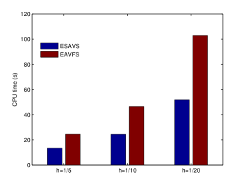
Fig. 1: CPU time of the two schemes for the soliton with different mesh sizes till $t=10$ under $\tau=0.001$.

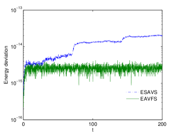
Fig. 2: The energy deviation with $h=\tau=0.1$ over the time interval $t\in[0,200]$.

Then, we apply the proposed scheme to solve the following two dimensional nonlinear sine-Gordon equation

$$\partial_{tt}u-\partial_{xx}u-\partial_{yy}u+\sin(u)=0,\ (x,y)\in\mathbb{R}^{2},\ t>0,$$

with initial conditions [11]

$$u(x,y,0)=4\tan^{-1}\left[\exp\left(\frac{4-\sqrt{(x+3)^{2}+(y+7)^{2}}}{0.436}\right)\right],$$

$$u_{t}(x,y,0)=\frac{4.13}{\cosh\left(\frac{4-\sqrt{(x+3)^{2}+(y+7)^{2}}}{0.436}\right)},\ (x,y)\in\mathbb{R}^{2}.$$

We take computational domain $\Omega=[-30,10]^{2}$ with a periodic boundary condition and choose the parameter $C_{0}=0$. In Fig. 3, we carry out comparison on the computational cost between two schemes by refining the mesh size gradually. It is clear to see that the cost of EAVFS is more expensive. Moreover, as the refinement of mesh sizes, the advantage of ESAVS emerges, which implies that our scheme is more preferable for large scale simulations than the EAVFS. Fig. 4 shows the collision precisely among four expanding circular ring solitons which are in good agreement with those given in Refs. [11, 40]. Here, we should note that, following Refs. [11, 40], the solution includes the extension across $x=-10$ and $y=-10$ by symmetry properties of the problem, and the numerical solution in terms of $\sin(u/2)$ instead of $u$ is displayed. Moverover, we also calculate the energy deviation for the two schemes over the time interval $t\in[0,100]$ and plot it in Fig. 5. As is clear, our scheme is comparable with the EAVFS.

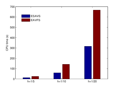
Fig. 3: CPU time of the two schemes for the soliton with different mesh sizes till $t=1$ under $\tau=0.01$.

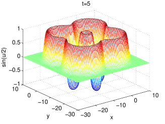
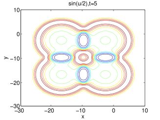
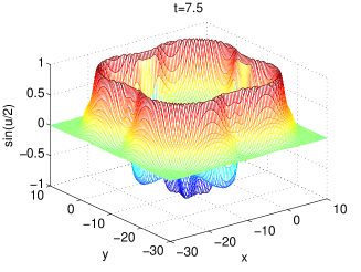
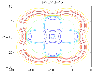
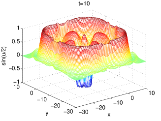
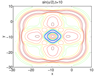
Fig. 4: Collision of four ring solitons (mesh plot (left) and contour plot (right)) in terms of $\sin(u/2)$ at times $t=0,2.5,5,7.5,10$ with $h=0.2$ and $\tau=0.1$.

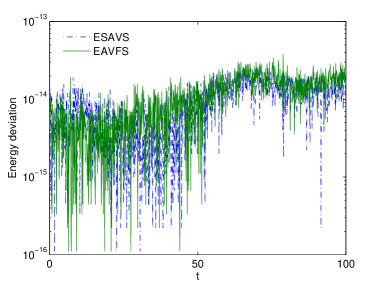
Fig. 5: The energy deviation over the time interval $t\in[0,100]$ with $h=0.2$ and $\tau=0.1$.

Finally, we consider the two dimensional nonlinear Klein-Gordon equation, as follows

$$\partial_{tt}u-\partial_{xx}u-\partial_{yy}u+u^{3}=0,\ (x,y)\in\mathbb{R}^{2},\ t>0,$$

with initial conditions

$$u(x,y,0)=2\text{sech}(\cosh(x^{2}+y^{2})),\ u_{t}(x,y,0)=0,\ (x,y)\in\mathbb{R}^{2}.$$

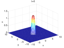
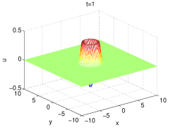
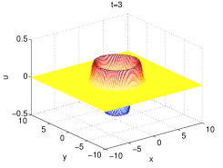
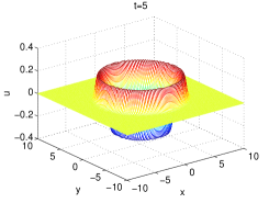
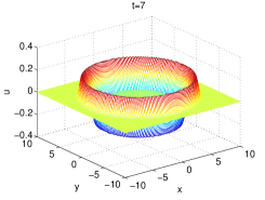
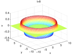
Fig. 6: The Snapshots of numerical solution at times $t=0,1,3,5,7,8$ with $h=\tau=0.1$.

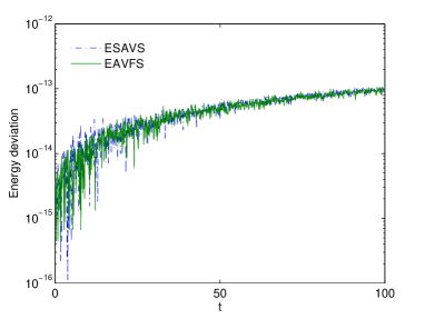
Fig. 7: The energy deviation over the time interval $t\in[0,100]$ with $h=\tau=0.1$.

We set the computational domain $\Omega=[-10,10]^{2}$ with a periodic boundary condition and take the parameter $C_{0}=0$. Fig. 6 presents the initial condition as well as numerical solutions at different times, which shows the expansion and propagation of the initial soliton to the whole domain until getting the boundary at $t=8$. The long time energy deviation of the two schemes is displayed in Fig. 7, which behaves similarly as that of Fig. 5. Here, we omit the comparison of the two schemes for the CPU time. This is because the obtained results behave similarly as that of Fig. 3.

5.2 Nonlinear Schrödinger equation

In this subsection, we focus on the nonlinear Schrödinger equation (NLSE) given as follows

$$\left\{\begin{aligned} &\text{i}\partial_{t}u({\bm{x}},t)+\Delta u({\bm{x}},t)+\beta|u({\bm{x}},t)|^{2}u({\bm{x}},t)=0,\ {\bm{x}}\in\mathbb{R}^{d},\\ &u({\bm{x}},0)=u_{0}({\bm{x}}),\ {\bm{x}}\in\mathbb{R}^{d},\end{aligned}\right.$$ (5.2)

where $\text{i}=\sqrt{-1}$ is the complex unit, $t$ is time variable, ${\bm{x}}\in\mathbb{R}^{d}$ is the spatial variable, $u:=u({\bm{x}},t)$ is the complex-valued wave function, $\Delta$ is the usual Laplace operator, and $\beta$ is a given real constant. The NLSE (5.2) conserves Hamiltonian energy

$$E(t):=\int_{\mathbb{R}^{d}}\Big{(}-|\nabla u({\bm{x}},t)|^{2}+\frac{\beta}{2}|u({\bm{x}},t)|^{4}\Big{)}d{\bm{x}}=E(0),\ t\geq 0.$$ (5.3)

For simplicity, we take the one dimensional case i.e. $d=1$ in (5.2) as example and set the computational domain $\Omega=[a,b]$ with periodic condition boundary. We then let $q:=q(t)=\sqrt{(|u|^{4},1)+C_{0}}$, and rewrite the energy functional (5.3) as

$$E(t):=\int_{\Omega}\big{(}-|\nabla u|^{2}\big{)}d{x}+\frac{\beta}{2}q^{2}-\frac{\beta}{2}C_{0}=E(0),\ t\geq 0.$$ (5.4)

According to the SAV reformulation, we obtain the following equivalent system

$$\left\{\begin{aligned} &\partial_{t}u=\text{i}\big{(}\Delta u+\beta\frac{|u|^{2}u}{\sqrt{(|u|^{4},1)+C_{0}}}q\big{)},\\ &\partial_{t}q=\frac{(|u|^{2}u,\partial_{t}u)+(\partial_{t}u,|u|^{2}u)}{\sqrt{(|u|^{4},1)+C_{0}}},\end{aligned}\right.$$ (5.5)

with the consistent initial condition

$$u({x},t=0)=u_{0}({x}),\ q(t=0)=\sqrt{(|u_{0}({x})|^{4},1)+C_{0}},\ x\in\Omega,$$ (5.6)

and a periodic condition boundary.

Instead of the finite difference method for discretization of the spatial derivative in (5.5), we use the standard Fourier pseudo-spectral method. Actually, the Laplace operator $\Delta$ is approximated by discrete Fourier transform (DFT) as

$$D_{2}=F^{H}\Lambda F,$$

where

$$\Lambda=-\Big{(}\frac{2\pi}{b-a}\Big{)}^{2}\text{\rm diag}\Big{[}0^{2},1^{2},\cdots,\big{(}\ \frac{N}{2}\big{)}^{2},\big{(}-\frac{N}{2}+1\big{)}^{2},\cdots,(-2)^{2},(-1)^{2}\Big{]}.$$

We let $u_{j}^{n}$ be the numerical approximation of $u(x_{j},t_{n})$ for $j=0,1,\cdots,N$ and $n=0,1,2,\cdots$; denote $u^{n}$ as the solution vector at $t=t_{n}$. Then, by an argument similar to the scheme (4.4)-(4.5) to system (5.5), we have

$$\left\{\begin{aligned} &u^{n+1}=\exp(\text{i}\tau D_{2})u^{n}+\text{i}\beta\tau\int_{0}^{1}\exp(\text{i}\tau D_{2}(1-\xi))d\xi\frac{|\hat{u}^{n+\frac{1}{2}}|^{2}\hat{u}^{n+\frac{1}{2}}q^{n+\frac{1}{2}}}{\sqrt{\langle|\hat{u}^{n+\frac{1}{2}}|^{4},{\bm{1}}\rangle_{l^{2}}+C_{0}}},\\ &q^{n+1}=q^{n}+\frac{\langle|\hat{u}^{n+\frac{1}{2}}|^{2}\hat{u}^{n+\frac{1}{2}},u^{n+1}-u^{n}\rangle_{l^{2}}+\langle u^{n+1}-u^{n},|\hat{u}^{n+\frac{1}{2}}|^{2}\hat{u}^{n+\frac{1}{2}}\rangle_{l^{2}}}{\sqrt{\langle|\hat{u}^{n+\frac{1}{2}}|^{4},{\bm{1}}\rangle_{l^{2}}+C_{0}}},\end{aligned}\right.$$ (5.7)

for $n=1,2,\cdots$. The initial condition (5.6) is discretized as

$$u_{j}^{0}=u_{0}(x_{j}),\ q^{0}=\sqrt{\langle|u^{0}|^{4},{\bm{1}}\rangle_{l^{2}}+C_{0}},\ j=0,1,2,\cdots,N.$$

Remark 5.1.

Note that the proposed scheme (5.7) is a three level scheme and we obtain ${u}^{1}$ and $q^{1}$ by using ${u}^{0}$ instead of $\hat{u}^{\frac{1}{2}}$ for the first step.

Theorem 5.1.

The proposed scheme (5.7) preserves the following modified energy

$${E}_{h}^{n+1}=E_{h}^{n},\ E_{h}^{n}=\langle-D_{2}u^{n},u^{n}\rangle_{l^{2}}-\frac{\beta}{2}(q^{n})^{2}-\frac{\beta}{2}C_{0}.$$

Proof.

The proof is similar to Theorem 4.1, thus, for brevity, we omit it.

Next, we show that the above scheme can be solved efficiently. Eqs. (5.7) can be rewritten as

$$u^{n+1}=\exp(\text{i}\tau D_{2})u^{n}+\phi\gamma^{n}q^{n+\frac{1}{2}},$$ (5.8)

$$q^{n+\frac{1}{2}}=\frac{1}{2}\langle\gamma^{n},u^{n+1}\rangle_{l^{2}}+\frac{1}{2}\langle u^{n+1},\gamma^{n}\rangle_{l^{2}}+q^{n}-\frac{1}{2}\langle\gamma^{n},u^{n}\rangle_{l^{2}}-\frac{1}{2}\langle u^{n},\gamma^{n}\rangle_{l^{2}},$$ (5.9)

where

$$\phi=\text{i}\beta\tau\int_{0}^{1}\exp(\text{i}\tau D_{2}(1-\xi))d\xi,\ \gamma^{n}=\frac{|\hat{u}^{n+\frac{1}{2}}|^{2}\hat{u}^{n+\frac{1}{2}}}{\sqrt{\langle|\hat{u}^{n+\frac{1}{2}}|^{4},{\bm{1}}\rangle_{l^{2}}+C_{0}}}.$$

Then, by eliminating $q^{n+\frac{1}{2}}$ in (5.8), we have

$$u^{n+1}=\frac{1}{2}\phi\gamma^{n}\langle\gamma^{n},u^{n+1}\rangle_{l^{2}}+\frac{1}{2}\phi\gamma^{n}\langle u^{n+1},\gamma^{n}\rangle_{l^{2}}+b^{n},$$ (5.10)

where

$$b^{n}=\exp(\text{i}\tau D_{2})u^{n}+\phi\gamma^{n}q^{n}-\frac{1}{2}\phi\gamma^{n}\langle\gamma^{n},u^{n}\rangle_{l^{2}}-\frac{1}{2}\phi\gamma^{n}\langle u^{n},\gamma^{n}\rangle_{l^{2}}.$$

We take the inner product of (5.10) with $\gamma^{n}$ and have, respectively,

$$\Big{(}1-\frac{1}{2}\langle\gamma^{n},\phi\gamma^{n}\rangle_{l^{2}}\Big{)}\langle\gamma^{n},u^{n+1}\rangle_{l^{2}}-\frac{1}{2}\langle\gamma^{n},\phi\gamma^{n}\rangle_{l^{2}}\langle u^{n+1},\gamma^{n}\rangle_{l^{2}}=\langle\gamma^{n},b^{n}\rangle_{l^{2}},$$ (5.11)

$$-\frac{1}{2}\langle\phi\gamma^{n},\gamma^{n}\rangle_{l^{2}}\langle\gamma^{n},u^{n+1}\rangle_{l^{2}}+\Big{(}1-\frac{1}{2}\langle\phi\gamma^{n},\gamma^{n}\rangle_{l^{2}}\Big{)}\langle u^{n+1},\gamma^{n}\rangle_{l^{2}}=\langle b^{n},\gamma^{n}\rangle_{l^{2}}.$$ (5.12)

Eqs. (5.11) and (5.12) form a $2\times 2$ linear system for the unknowns $\Big{(}\langle\gamma^{n},u^{n+1}\rangle_{l^{2}},\langle u^{n+1},\gamma^{n}\rangle_{l^{2}}\Big{)}^{T}$.

Solving $\Big{(}\langle\gamma^{n},u^{n+1}\rangle_{l^{2}},\langle u^{n+1},\gamma^{n}\rangle_{l^{2}}\Big{)}^{T}$ from the $2\times 2$ linear system (5.11) and (5.12), and $u^{n+1}$ is then updated from (5.10). Subsequently, $q^{n+\frac{1}{2}}$ is obtained by (5.9). Finally, we have $q^{n+1}=2q^{n+\frac{1}{2}}-q^{n}$.

Remark 5.2.

In addition, by an argument similar to Remark 4.3, we can deduce that

$$\exp(\text{\rm i}\tau D_{2})=F^{H}\exp(\text{\rm i}\tau\Lambda)F,\ \int_{0}^{1}\exp(\text{\rm i}\tau D_{2}(1-\xi))d\xi=F^{H}\Sigma F,$$

where

$$\Sigma=\text{\rm diag}\Big{[}1,\frac{\exp(\text{\rm i}\tau\lambda_{1})-1}{\text{\rm i}\tau\lambda_{1}},\cdots,\frac{\exp(\text{\rm i}\tau\lambda_{N-1})-1}{\text{\rm i}\tau\lambda_{N-1}}\Big{]}.$$

We repeat the time step refinement test first and choose the parameter $C_{0}=0$ and $\beta=2$. The one dimensional Schrödinger equation (5.2) admits the analytical solution

$$u(x,t)=\text{sech}(x-4t)\exp(2\text{i}x-3\text{i}t),\ x\in\mathbb{R}.$$

We choose the analytical solution at $t=0$ as initial condition and set the computational domain $\Omega=[-40,40]$ with a periodic boundary. To test the temporal discretization errors of the two numerical schemes, we fix the Fourier node $4096$ such that the spatial discretization errors are negligible.

The $L^{2}$ errors and $L^{\infty}$ errors in numerical solution of $u$ at $t=1$ are calculated using two numerical schemes with various time steps, and the results are displayed in Fig. 8. In Fig. 9, we show the global $L^{2}$ errors and $L^{\infty}$ errors of $u$ versus the CPU time using the two different schemes at $t=1$. From Figs. 8 and 9, we can draw the following observations: (i) all schemes have second order accuracy in time; (ii) the error provided by the EAVFS is smallest, and the one provided by the proposed scheme has the same order of magnitude as the one of the ESAV scheme; (iii) for a given global error, the cost of the EAVFS is more expensive than the proposed scheme.

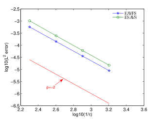
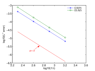
Fig. 8: Time step refinement tests using the two numerical schemes for the one dimensional Schrödinger equation.

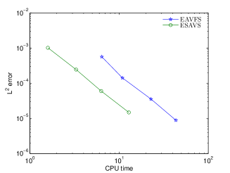
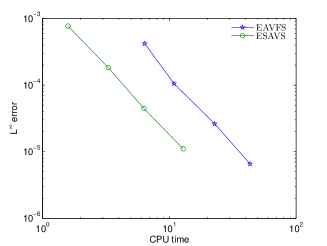
Fig. 9: The numerical error versus the CPU time using the two numerical schemes for the one dimensional Schrödinger equation.

To further investigate the energy-preservation of the proposed scheme, we provide the energy errors using the two numerical schemes for the one dimensional Schrödinger equation over the time interval $t\in[0,100]$ in Fig. 10, which shows that all two methods can exactly preserve the discrete energies.

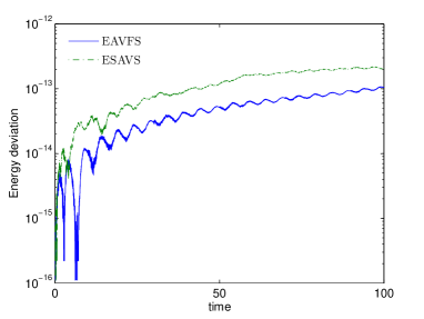
Fig. 10: The energy deviation using the two numerical schemes with time step $\tau=0.01$ and spatial collocation point $N=512$ for the one dimensional Schrödinger equation.

Next, we apply the proposed scheme to solve the two dimensional nonlinear Schrödinger equation which possesses the following analytical solution

$$u(x,y,t)=A\exp(\text{i}(k_{1}x+k_{2}y-\omega t)),\ \omega=k_{1}^{2}+k_{2}^{2}-\beta|A|^{2},\ (x,y)\in\Omega.$$

We choose the computational domain $\Omega=[0,2\pi]^{2}$ and take parameters $A=1,\ k_{1}=k_{2}=1$, $\beta=-1$ and $C_{0}=0$. We first test the temporal accuracy of the two numerical schemes by fixing the Fourier node $64\times 64$ such that the spatial discretization errors are negligible. The $L^{2}$ errors and $L^{\infty}$ errors in numerical solution of $u$ at $t=1$ calculated by using two numerical schemes with various time steps are shown in Fig. 11. Also, the global $L^{2}$ errors and $L^{\infty}$ errors of $u$ versus the CPU time using the two different schemes at $t=1$ are investigated in Fig. 12. Again, the numerical results indicate that two numerical schemes are second order in time and the proposed scheme is much cheaper than EAVFS.

Second, we present the discrete energies for the numerical solutions given by the ESAVS and EAVFS, respectively in Fig. 13. The numerical results show that the discrete energies can be exactly preserved, which are consistent with our theoretical result in Theorem 5.1.

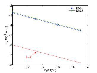
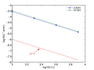
Fig. 11: Time step refinement tests using the two numerical schemes for the two dimensional Schrödinger equation.

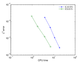
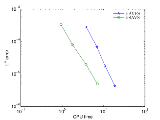
Fig. 12: The numerical error versus the CPU time using the two numerical schemes for the two dimensional Schrödinger equation.

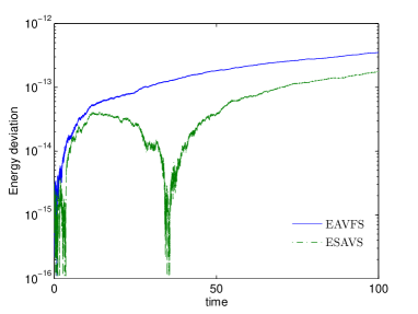
Fig. 13: The energy deviation using the two numerical schemes with time step $\tau=0.01$ and spatial collocation point $32\times 32$ for the two dimensional Schrödinger equation.

6 Concluding remarks

In this paper, we design a novel linearly implicit energy-preserving exponential scheme for the nonlinear Klein-Gordon equation and the nonlinear Schrödinger equation, respectively. The schemes were developed based on the exponential integrator in combination with the scalar auxiliary variable (SAV) technique and proved to preserve the discrete energy. Various numerical examples are carried out to illustrate theoretical analysis. Comparing with the exponential averaged vector filed scheme, the proposed scheme shows remarkable efficiency. Here, we should note that, compared with existing energy-preserving exponential schemes (e.g., see Refs. [30, 39]), the proposed method cannot preserve the discrete Hamiltonian energy. Thus, such trade-offs among methods should be more carefully investigated. In addition, to the best of our knowledge, the construction of higher order linearly implicit energy-preserving exponential schemes is still not available for conservative systems, which is an interesting topic for future studies.

References

- [1] L. Brugnano, G. Frasca Caccia, and F. Iavernaro. Energy conservation issues in the numerical solution of the semilinear wave equation. Appl. Math. Comput., 270:842–870, 2015.
- [2] L. Brugnano, F. Iavernaro, and D. Trigiante. Hamiltonian boundary value methods (energy preserving discrete line integral methods). J. Numer. Anal. Ind. Appl. Math., 5:17–37, 2010.
- [3] J. Cai and J. Shen. Two classes of linearly implicit local energy-preserving approach for general multi-symplectic Hamiltonian pdes. J. Comput. Phys., 401:108975, 2020.
- [4] W. Cai, C. Jiang, Y. Wang, and Y. Song. Structure-preserving algorithms for the two-dimensional sine-Gordon equation with Neumann boundary conditions. J. Comput. Phys., 395:166–185, 2019.
- [5] W. Cai, H. Li, and Y. Wang. Partitioned averaged vector field methods. J. Comput. Phys., 370:25–42, 2018.
- [6] E. Celledoni, D. Cohen, and B. Owren. Symmetric exponential integrators with an application to the cubic Schrödinger equation. Found. Comput. Math., 8:303–317, 2008.
- [7] E. Celledoni, V. Grimm, R. I. McLachlan, D. I. McLaren, D. O’Neale, B. Owren, and G. R. W. Quispel. Preserving energy resp. dissipation in numerical PDEs using the “Average Vector Field” method. J. Comput. Phys., 231:6770–6789, 2012.
- [8] W. Chen, W. Li, Z. Luo, C. Wang, and X. Wang. A stabilized second order exponential time differencing multistep method for thin film growth model without slope selection. arXiv preprint arXiv:1907.02234, 2019.
- [9] D. Cohen, E. Hairer, and C. Lubich. Conservation of energy, momentum and actions in numerical discretizations of non-linear wave equations. Numer. Math., 110:113–143, 2008.
- [10] M. Dahlby and B. Owren. A general framework for deriving integral preserving numerical methods for PDEs. SIAM J. Sci. Comput., 33:2318–2340, 2011.
- [11] K. Djidjeli, W. G. Price, and E. H. Twizell. Numerical solutions of a damped sine-Gordon equation in two space variables. J. Engrg. Math., 29:347–369, 1995.
- [12] Q. Du, L. Ju, X. Li, and Z. Qiao. Maximum principle preserving exponential time differencing schemes for the nonlocal Allen–Cahn equation. SIAM J. Numer. Anal., 57:875–898, 2019.
- [13] D. B. Duncan. Sympletic finite difference approximations of the nonlinear Klein-Gordon equation. SIAM J. Numer. Anal., 34:1742–1760, 1997.
- [14] D. Furihata and T. Matsuo. Discrete Variational Derivative Method: A Structure-Preserving Numerical Method for Partial Differential Equations. Chapman & Hall/CRC, Boca Raton, 2011.
- [15] Y. Gong, J. Cai, and Y. Wang. Some new structure-preserving algorithms for general multi-symplectic formulations of Hamiltonian PDEs. J. Comput. Phys, 279:80–102, 2014.
- [16] B. Guo and P. Pascual. Numerical solution of the sine-Gordon equation. Appl. Math. Comput., 18:1–14, 1986.
- [17] E. Hairer. Energy-preserving variant of collocation methods. J. Numer. Anal. Ind. Appl. Math., 5:73–84, 2010.
- [18] E. Hairer, C. Lubich, and G. Wanner. Geometric Numerical Integration: Structure-Preserving Algorithms for Ordinary Differential Equations. Springer-Verlag, Berlin, 2nd edition, 2006.
- [19] P. C. Hansen, J. G. Nagy, and D. P. O’leary. Deblurring Images: Matrices, Spectra, and Filtering, Chapter 4. SIAM, 2006.
- [20] J. Hersch. Contribution á la méthode des équations aux différences. Z. Angew. Math. Phys., 9:129–180, 1958.
- [21] N. J. Higham. Functions of Matrices: Theory and Computation. SIAM, Philadelphia, 2008.
- [22] M. Hochbruck, C. Lubich, and H. Selhofer. Exponential integrators for large systems of differential equations. SIAM J. Sci. Comput., 19:1552–1574, 1998.
- [23] M. Hochbruck and A. Ostermann. Exponential integrators. Acta Numer., 19:209–286, 2010.
- [24] J. Hong, S. Jiang, C. Li, and H. Liu. Explicit multi-symplectic methods for Hamiltonian wave equations. Commun. Comput. Phys., 2:662–683, 2007.
- [25] C. Jiang, W. Cai, and Y. Wang. A linearly implicit and local energy-preserving scheme for the sine-Gordon equation based on the invariant energy quadratization approach. J. Sci. Comput., 80:1629–1655, 2019.
- [26] C. Jiang, Y. Gong, W. Cai, and Y. Wang. A linearly implicit structure-preserving scheme for the Camassa-Holm equation based on multiple scalar auxiliary variables approach. arXiv:1907.00167 [math.NA], 2019.
- [27] L. Ju, X. Li, Z. Qiao, and H. Zhang. Energy stability and error estimates of exponential time differencing schemes for the epitaxial growth model without slope selection. Math. Comp., 87:1859–1885, 2018.
- [28] H. Li, Y. Wang, and M. Qin. A sixth order averaged vector field method. J. Comput. Math., 34:479–498, 2016.
- [29] S. Li and L. Vu-Quoc. Finite difference calculus invariant structure of a class of algorithms for the nonlinear Klein-Gordon equation. SIAM. J. Numer. Anal., 32:1839–1875, 1995.
- [30] Y. Li and X. Wu. Exponential integrators preserving first integrals or Lyapunov functions for conservative or dissipative systems. SIAM J. Sci. Comput., 38:A1876–A1895, 2016.
- [31] R. McLachlan. Symplectic integration of Hamiltonian wave equations. Numer. Math., 66:465–492, 1993.
- [32] R. I. McLachlan, G. R. W. Quispel, and N. Robidoux. Geometric integration using discrete gradients. Philos. Trans. R. Soc. A, 357:1021–1045, 1999.
- [33] L. Mei and X. Wu. Symplectic exponential Runge-Kutta methods for solving nonlinear Hamiltonian systems. J. Comput. Phys., 338:567–584, 2017.
- [34] Y. Miyatake and J. C. Butcher. A characterization of energy-preserving methods and the construction of parallel integrators for Hamiltonian systems. SIAM J. Numer. Anal., 54:1993–2013, 2016.
- [35] G. R. W. Quispel and D. I. McLaren. A new class of energy-preserving numerical integration methods. J. Phys. A: Math. Theor., 41:045206, 2008.
- [36] S. Reich. Multi-symplectic Runge-Kutta collocation methods for Hamiltonian wave equations. J. Comput. Phys., 157:473–499, 2000.
- [37] J. Shen, J. Xu, and J. Yang. The scalar auxiliary variable (SAV) approach for gradient. J. Comput. Phys., 353:407–416, 2018.
- [38] J. Shen, J. Xu, and J. Yang. A new class of efficient and robust energy stable schemes for gradient flows. SIAM Rev., 61:474–506, 2019.
- [39] X. Shen and M. Leok. Geometric exponential integrators. J. Comput. Phys., 382:27–42, 2019.
- [40] Q. Sheng, A. Q. M. Khaliq, and D. A. Voss. Numerical simulation of two-dimensional sine-Gordon solitons via a split cosine scheme. Math. Comput. Simulation, 68:355–373, 2005.
- [41] W. Shi, X. Wu, and J. Xia. Explicit multi-symplectic extended leap-frog methods for Hamiltonian wave equations. J. Comput. Phys., 231:7671–7694, 2012.
- [42] W. Tang and Y. Sun. Time finite element methods: a unified framework for numerical discretizations of ODEs. Appl. Math. Comput., 219:2158–2179, 2012.
- [43] B. Wang and X. Wu. The formulation and analysis of energy-preserving schemes for solving high-dimensional nonlinear Klein-Gordon equations. IMA J. Numer. Anal., 39:2016–2044, 2019.
- [44] Y. Wang, B. Wang, and M. Qin. Local structure-preserving algorithms for partial differential equations. Sci. China Ser. A, 51:2115–2136, 2008.
- [45] X. Wu and B. Wang. Recent Developments in Structure-Preserving Algorithms for Oscillatory Differential Equations. Springer, Singapore, 2018.
- [46] X. Yang, J. Zhao, and Q. Wang. Numerical approximations for the molecular beam epitaxial growth model based on the invariant energy quadratization method. J. Comput. Phys., 333:104–127, 2017.
- [47] F. Zhang, V. M. Pérez-García, and L. Vázquez. Numerical simulation of nonlinear schrödinger systems: a new conservative scheme. Appl. Math. Comput., 71:165–177, 1995.
- [48] J. Zhao, X. Yang, Y. Gong, and Q. Wang. A novel linear second order unconditionally energy stable scheme for a hydrodynamic-tensor model of liquid crystals. Comput. Methods Appl. Mech. Engrg., 318:803–825, 2017.
- [49] H. Zhu, L. Tang, S. Song, Y. Tang, and D. Wang. Symplectic wavelet collocation method for Hamiltonian wave equations. J. Comput. Phys., 229:2550–2572, 2010.