LiDARTag: A Real-Time Fiducial Tag System for Point Clouds

Abstract

Image-based fiducial markers are useful in problems such as object tracking in cluttered or textureless environments, camera (and multi-sensor) calibration tasks, and vision-based simultaneous localization and mapping (SLAM). The state-of-the-art fiducial marker detection algorithms rely on the consistency of the ambient lighting. This paper introduces LiDARTag, a novel fiducial tag design and detection algorithm suitable for light detection and ranging (LiDAR) point clouds. The proposed method runs in real-time and can process data at 100 Hz, which is faster than the currently available LiDAR sensor frequencies. Because of the LiDAR sensors’ nature, rapidly changing ambient lighting will not affect the detection of a LiDARTag; hence, the proposed fiducial marker can operate in a completely dark environment. In addition, the LiDARTag nicely complements and is compatible with existing visual fiducial markers, such as AprilTags, allowing for efficient multi-sensor fusion and calibration tasks. We further propose a concept of minimizing a fitting error between a point cloud and the marker’s template to estimate the marker’s pose. The proposed method achieves millimeter error in translation and a few degrees in rotation. Due to LiDAR returns’ sparsity, the point cloud is lifted to a continuous function in a reproducing kernel Hilbert space where the inner product can be used to determine a marker’s ID. The experimental results, verified by a motion capture system, confirm that the proposed method can reliably provide a tag’s pose and unique ID code. The rejection of false positives is validated on the Google Cartographer indoor dataset and the Honda H3D outdoor dataset. All implementations are coded in C++ and are available at: https://github.com/UMich-BipedLab/LiDARTag.

I Introduction

Artificial landmark systems, referred to as fiducial markers, have been designed for automatic detection via specific type of sensors such as cameras [1, 2, 3, 4, 5, 6]. The marker usually consists of a payload, that is, a pattern that makes individual markers uniquely distinguishable, and a boundary surrounding the payload that is designed to assist with isolating the payload from its background. Their supporting algorithms typically consist of modules to detect the marker, decode its payload, and estimate the pose. Such artificial landmarks have been successfully used in computer vision, augmented reality [1] and simultaneous localization and mapping (SLAM) [7].

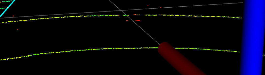
(a)

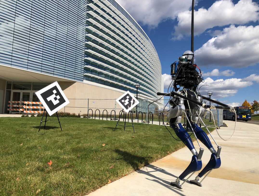
(b)

Figure 1: LiDAR-based markers can be used in tandem with camera-based markers to address the issue of images being sensitive to ambient lighting. This figure shows a visualization of LiDARTags of two different sizes in a full point cloud scan.

Images are sensitive to lighting variations, and therefore, visual fiducial markers rely heavily on the assumption of illumination consistency. As such, when lighting changes rapidly throughout a scene, the detection of visual markers can fail. Alternatively, light detection and ranging devices (LiDARs) are robust to illumination changes due to the active nature of the sensor. In particular, rapid changes in the ambient lighting do not affect the detection of features in point clouds returned by a LiDAR. Unfortunately, however LiDARs cannot detect the fiducial markers designed for cameras. Hence, to utilize the advantages of both sensor modalities, a new type of fiducial marker that can be perceived by both LiDARs and cameras is required. Such a new marker can enable applications such as multi-sensor fusion and calibration tasks involving visual and LiDAR data [8]. Designing such fiducial markers is challenging due to inherent LiDAR properties such as sparsity, lack of structure and the varying number of points in a scan. In particular, the fact that an individual LiDAR return has no fixed spatial relation to neighboring returns makes it difficult to isolate a fiducial marker within a point cloud.

In this paper, we propose a novel and flexible design of a fiducial tag system, called LiDARTag, as shown in Figure 1. A system is further developed to detect LiDARTags with various sizes and to estimate their poses. Point clouds are represented as functions in a Reproducing Kernel Hilbert Space (RKHS) [9] to decode their IDs. The whole system can run in real-time (over 100 Hz), which is even faster than currently available data rates of LiDAR sensors. The proposed LiDARTag can be perceived by both RGB-cameras and point clouds. In [8, 10], the authors used LiDARTags in a LiDAR-camera calibration pipeline as a means to extract the LiDAR returns on the tag. The LiDARTag system was not used to decode a payload nor to estimate pose. LiDARTags have been successfully used for LiDAR-camera calibration [8, 10]. It can be further applied to SLAM systems for robot state estimation and loop closures. Additionally, it can help improve human-robot interaction, allowing humans to give commands to a robot by showing an appropriate LiDARTag. However, the proposed system utilizes the intensity measurement of a LiDARTag to decode its ID. Therefore, LiDARs with stable (good) intensity readings are required. In particular, the present work has the following contributions:

1. We propose a novel and flexible fiducial marker for point clouds, LiDARTag, that is compatible with existing image-based fiducial marker systems, such as AprilTag.

2. We develop a robust real-time method to estimate the pose of a LiDARTag. The optimal pose estimate minimizes an $L_{1}$-inspired fitting error between the point cloud and the marker’s template of known geometry.

3. To address the sparsity of LiDAR returns, we lift a point cloud to a continuous function in an RKHS and use the inner product structure to determine a marker’s ID among a pre-computed function dictionary.

4. We present performance evaluations of the LiDARTag where ground truth data are provided by a motion capture system. We also extensively analyze each step in the system with spacious outdoor and cluttered indoor environments. Additionally, we report the rate of false positives validated on the indoor Google Cartographer [11] dataset and the outdoor Honda H3D dataset [12].

5. We provide open-source implementations for the physical design of the proposed LiDARTag and all of the associated software for using them, in C++ and Robot Operating System (ROS) [13]; see https://github.com/UMich-BipedLab/LiDARTag [14].

The remainder of this paper is organized as follows. Section II presents a summary of the related work. Section III explains the tag design. Tag detection and pose estimation are discussed in Section IV and Section V. The construction of continuous functions and ID decoding are introduced in Section VI. Experimental evaluations of the proposed LiDARTags are presented in Section VII. Finally, Section VIII concludes the paper and provides suggestions for future work.

II Related Work

Fiducial marker systems were originally developed and used for augmented reality applications [1, 2] and have been widely used for object detection and tracking and pose estimation [15]. Due to their uniqueness and fast detection rate, they are also often used to improve Simultaneous Localization And Mapping (SLAM) systems [7]. Because of automatic detection, the camera-based markers are often used to extract features for cameras in target-based LiDAR-camera calibration [8, 16, 17], and the proposed algorithm can provide a means to extract features for LiDARs. To the best of our knowledge, there are no existing fiducial markers for point clouds. Among the many popular camera-based fiducial markers are ARToolKit [1], ARTag [2], AprilTag 1-3 [3, 4, 5], and CALTag [18].

In the following, we review some recent and well-known fiducial markers for cameras. ARTag [2] [19] uses a 2D barcode to make decoding easier. AprilTag 1-3 [3, 4, 5] introduced a lexicode-based [20] tag generation method in order to reduce false positive detection. ChromaTag [6] proposes color gradients to speed up the detection process. RuneTag [21] uses rings of dots to improve occlusion robustness and more accurate camera pose estimation. CCTag [22] adopts a set of rings to enhance blur robustness. More recently, LFTag [23] has taken advantage of topological markers, a kind of uncommon topological pattern, to improve longer detection range. This also enables the decoding of markers with high distortion, and these markers can be flexibly laid down. While there are some fiducial markers using deep learning technique [24, 25], to date, all of those detectors, still only work on cameras.

There are several deep-learning-based object detection architectures for LiDAR point cloud. Most of the methods for 3D object detection deploy a voxel grid representation [26, 27, 28]. Recently, [29, 27, 30] have sought to improve feature representation with 3D convolution networks, which require expensive computation. Similar to proposed methods for 2D objects [31, 32, 33, 34, 35], the proposed methods for 3D objects generate a set of 3D boxes in order to cover most of the objects in 3D space. However, most detectors are limited to specific categories and none of these detectors or proposed methods has adequately addressed rotation, perspective transformations, or domain adoption.

Remark 1.

As mentioned above, there exist several deep-learning-based object detectors trained on large-scale LiDAR datasets [36, 37, 38]. These detectors are trained on limited categories in a specific dataset, and if the training and testing data are not consistent, the inference process could fail. They would have to be retrained on new data in order to be viable for our LiDARTag. Another option could be to design our own detector and train on our own datasets rather than using existing detectors. However, there is no guarantee that the resulting detector would work for varied scenes spanning from a cluttered laboratory to spacious outdoor environments. Additionally, the existing detectors rely on powerful graphics processing units (GPUs) and they are thus not suitable for lightweight mobile robots. On the other hand, the detector proposed in this paper is robust to general scenarios and achieves satisfactory results in practice. Deep-learning-based methods, however, are interesting future work and are discussed in Sec. VIII.

III Tag Design and LiDAR Characteristics

This section describes some essential points to consider when designing and using a LiDAR-based tag system. In particular, this section addresses how the unstructured point cloud from a LiDAR results in different considerations in the selection of a marker versus those used with a camera.

III-A LiDAR Point Clouds vs Camera Images

Pixel arrays (i.e., an image) from standard RGB-cameras of different resolutions are very structured, with the pixels arranged in a uniform (planar) grid, and each image having a fixed number of data points. A LiDAR returns $(x,y,z)$ coordinates of 3D points lying on the surface of objects as well as the intensity, which relies on the reflectivity/material of the object. The reflectivity is measured at the wavelength used by the LiDAR. Some LiDARs also provide beam numbers. The resulting 3D point clouds are typically referred to as “unstructured” because:

• The number of returned points varies for each scan and for each beam. In particular, LiDAR returns are not uniformly distributed in angle or distance.

• As shown in Fig. 2, high contrast between adjacent regions of a target’s surface can result in missing returns and in varying spaces between returns.

• When used outdoors, the number of returned points is also influenced by environmental factors such as weather, especially temperature.

Consequently, as opposed to an image, there is no fixed geometric relationship between the index numbers of returns from two different beams in a multi-beam LiDAR. A further difference is the density of the collected data; currently, basic cameras provide many more data points for a given surface size at a given distance than even high-end LiDARs. These summarized differences have an impact on how one approaches the design of a LiDAR-based tag system vs. a camera-based tag system.

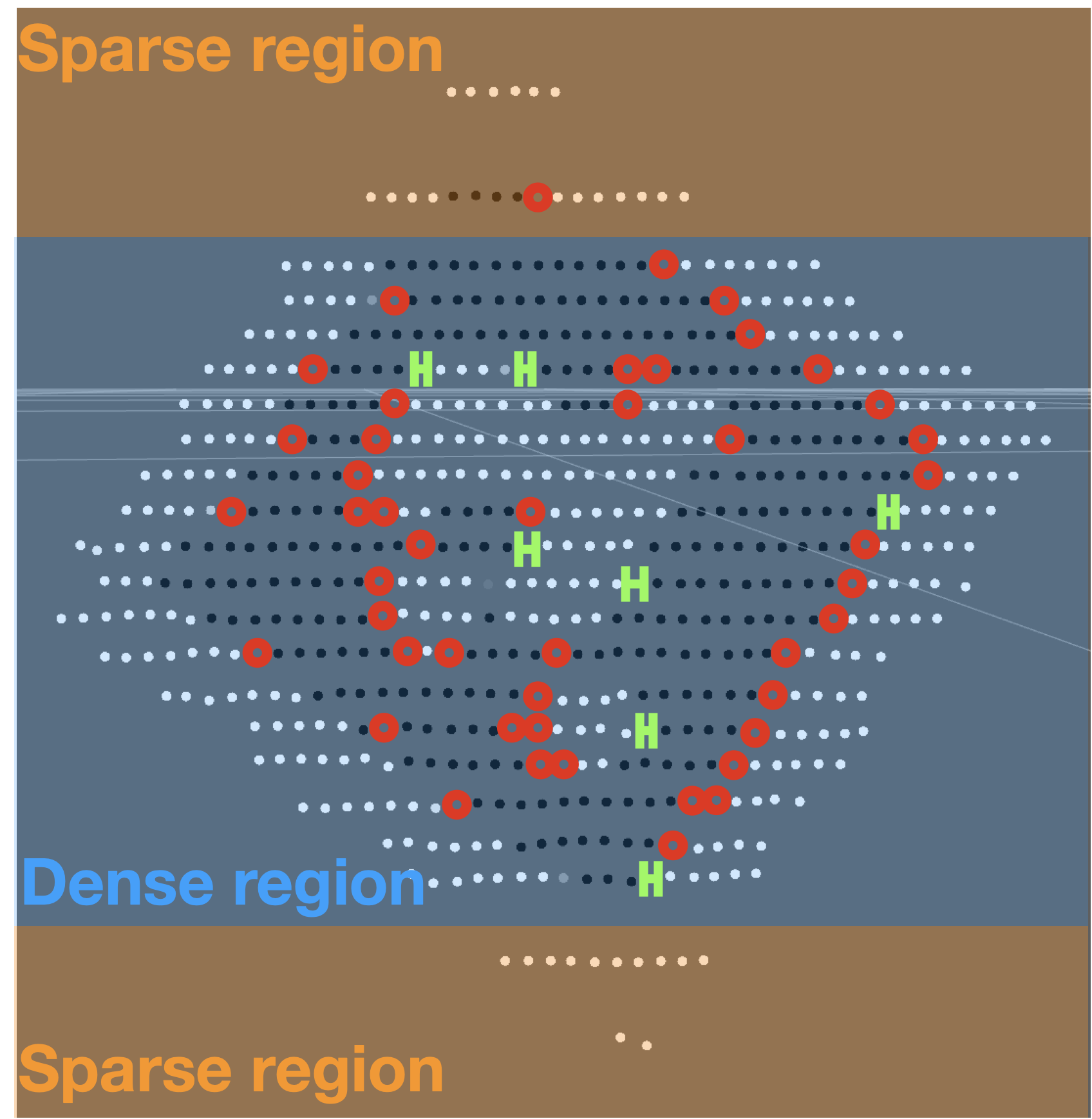
(a)

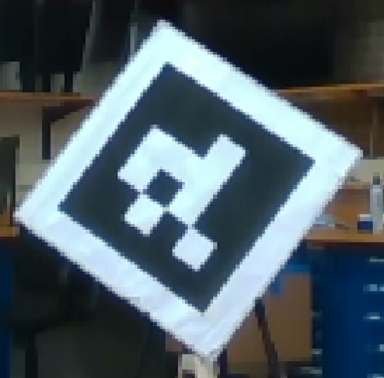
(b)

Figure 2: This figure illustrates the unstructured nature of a LiDAR-point-cloud return (left) for a planar surface with black and white squares (right). On the left, the black and white dots are lower reflectivity and higher reflectivity, respectively. The sparse region of the LiDAR is indicated in light yellow and the dense region is marked in light blue. The returns are more irregular at the black-white transitions. Red circles indicate missing returns and green bars highlight larger gaps between returned points.

III-B Tag Placement and Design

As mentioned in Sec. III-A, a return from a typical LiDAR consists of an $(x,y,z)$ measurement, an intensity value $i$, and a beam number (often called ring number, $r$). In this paper, we propose exploiting the relative accuracy of a LiDAR’s distance measurement to determine “features” when seeking to isolate a LiDARTag in a 3D point cloud (see Sec. IV) and associating the isolated LiDARTag points with a continuous function to decode the marker’s payload (see Sec. VI).

III-B1 Tag design

A LiDARTag is assumed to consist of a planar fiducial marker rigidly attached to a 3D object, as shown in Fig. 3a. In particular, the marker shows different intensity values when illuminated by a LiDAR. As indicated in Sec. III-A, intensity relies on how a LiDAR measures the reflectivity of an object. Most types of fiducial markers for camera-based systems could be adapted for use in LiDAR-based systems as long as the payload is composed of differing reflectivities and is placed inside the region highlighted in yellow in Fig. 3b. Figure 3c shows an example of an AprilTag used as a LiDARTag. In our experiments, we print the tags from a regular printer and a poster machine. Because fiducial markers are usually printed from a printer, however, markers with two colors such as AprilTag 1-3 [3, 4, 5], ARTag [2, 19], InterSense [40], CyberCode [41], or CALTag [18] can be most easily adapted for use in our LiDARTag system, while Cho et.al [42] with multi-color cannot.

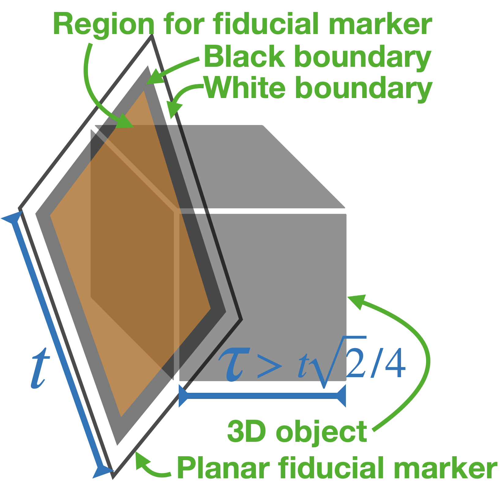
(a)

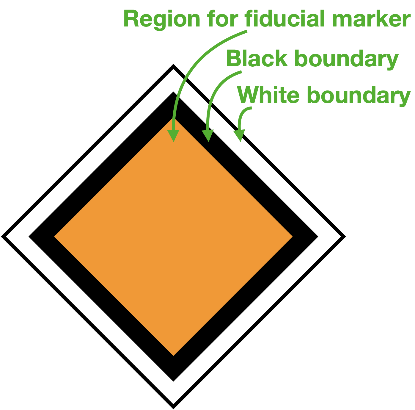
(b)

(c)

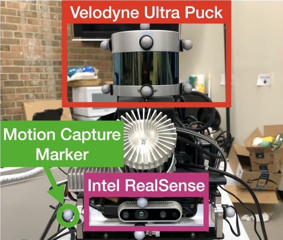
(d)

Figure 3: LABEL:sub@fig:3dtag illustrates a LiDARTag consisting of two parts: a 3D object with a rigidly attached, planar fiducial marker where $t$ and $h$ are the marker size and height of the object respectively. LABEL:sub@fig:tag_explain shows the marker should be placed inside the yellow region and LABEL:sub@fig:MarkerExample illustrates an example of AprilTag being used as a LiDARTag. LABEL:sub@fig:torso is the sensor setup consisting of a LiDAR, a camera and several motion capture markers.

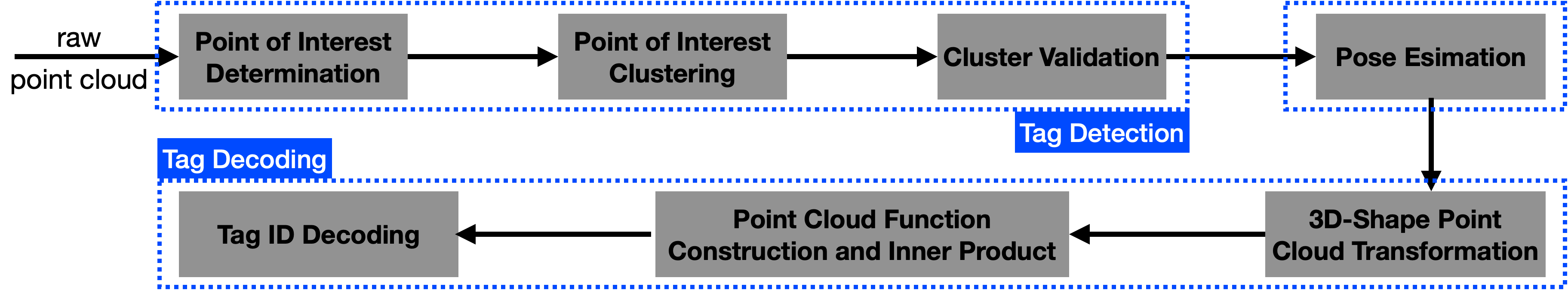
Figure 4: The system contains three parts: tag detection, pose estimation, and tag decoding. The detection step takes an entire LiDAR scan (up to 120,000 points from a 32-Beam Velodyne ULTRA Puck LiDAR) and outputs collections of likely payload points of the LiDARTags. Next, a tag’s optimal pose minimizes the $L_{1}$-inspired cost in (8), though the rotation of the tag about a normal vector to the tag may be off by $\pm 90^{\circ}$ or $180^{\circ}$ and will be resolved in the decoding process. The tag’s ID is decoded with a function library inspired by [43, 44]. The decoded tag removes the rotation ambiguity about the normal.

For this initial study, we employ AprilTag3 as our fiducial markers. Furthermore, within the AprilTag3 family of markers, we select tag16h6c5, that is, a tag encoding 16 bits (i.e., 16 black or white squares), with a minimum Hamming distance of 6, and a complexity of 5. The Hamming distance measures the minimum number of bit changes (e.g., bit errors) required to transform one string of bits into the other. For example, the length-7 strings $``1011111"$ and $``1001011"$ have a Hamming distance of 2, whereas $``1011111"$ and $``1001010"$ have a Hamming distance of 3. The significance is that a lexicode with a minimum Hamming distance $h$ can detect $h/2$ bit errors and correct up to $\lfloor(h-1)/2\rfloor$ bit errors [20]. The complexity of an AprilTag is defined as the number of rectangles required to generate the tag’s 2D pattern. For example, a solid pattern requires just one rectangle, whereas, a white-black-white stripe would need two rectangles (first draw a large white rectangle; then draw a smaller black rectangle). For further details, we refer the reader to the coding discussion in Olson [3].

Remark 2.

One may argue that other members of the AprilTags3 family, such as tag49h15c15, tag36h11c10, tag36h10c10, and tag25h10c8, would be more appropriate. For example, including more bits tends to increase the number of distinct tags in a family, while a larger Hamming distance reduces false positives. However, for tags of the same physical size and the same distance from the sensor, more bits means fewer returns per square and a higher error rate for individual squares.

III-B2 Tag placement

In Fig. 3a, let $t$ be the tag size and $h$ be the thickness of the 3D object. The 3D object is assumed to have $t\sqrt{2}/4$ clearance around it, and the first LiDAR ring hitting at a LiDARTag is above $3/4$ of the LiDARTag, see Sec. IV-B. In particular, the fiducial marker can be attached to a wall as long as the condition, $h>t\sqrt{2}/4$, in Fig. 3a is met. Finally, it is not recommended to orient the marker like a square due to the quantization error inherited in LiDAR sensors, see [8, Sec. II].

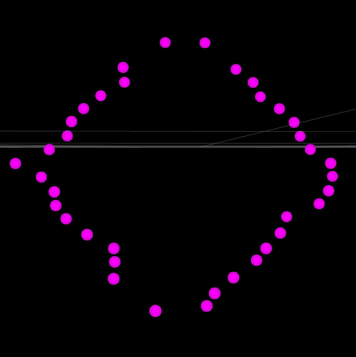
(a)

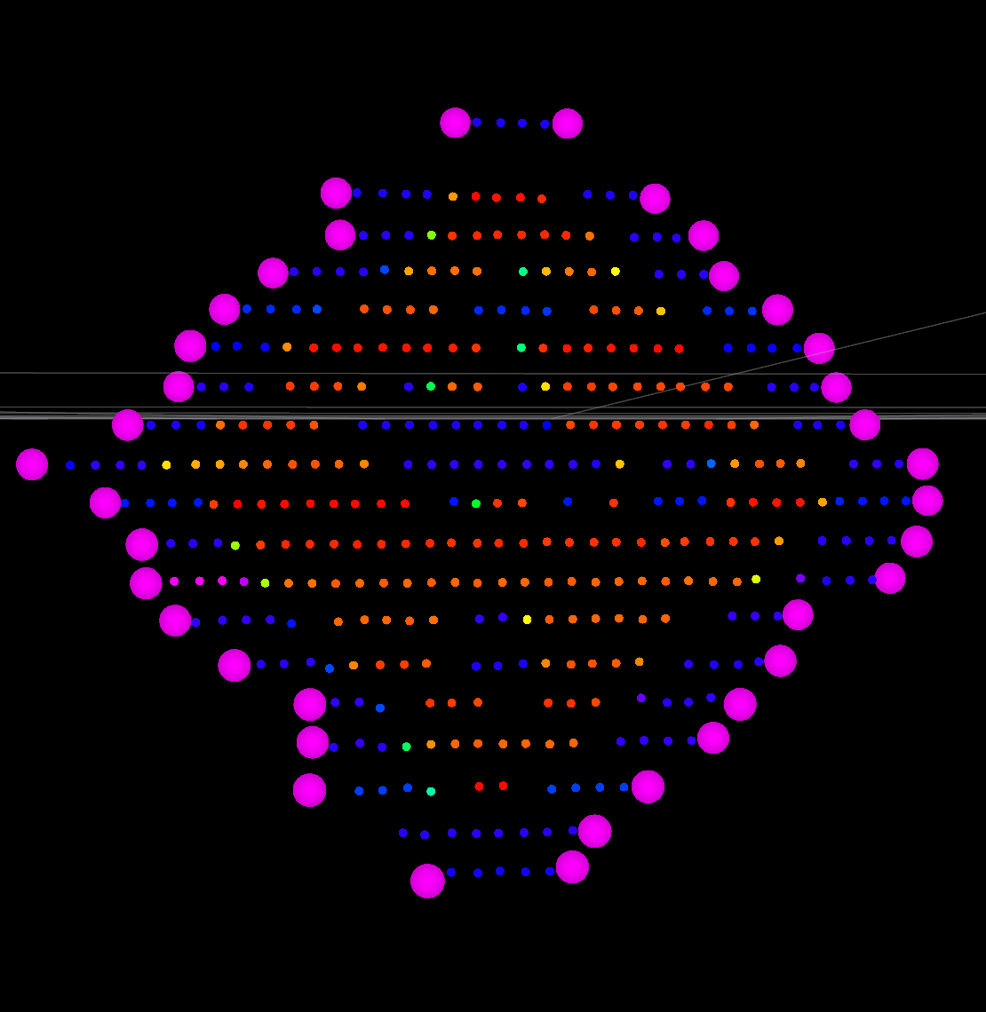
(b)

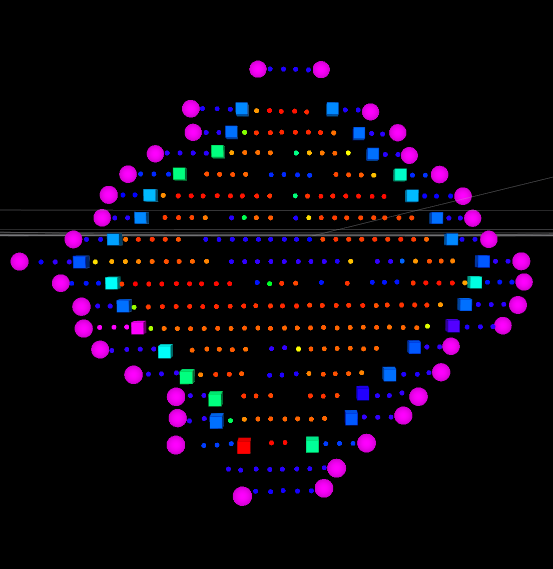
(c)

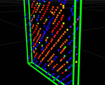
(d)

Figure 5: Intermediate steps of the LiDARTag system. The system takes a full scan point cloud and applies feature detection as defined in (1) and associates the features into clusters (magenta spheres), as shown in LABEL:sub@fig:edges. Using the features, the clusters are filled from the original scan (different color dots stand for different intensity values) as shown in LABEL:sub@fig:filled. Later, boundary points (indicated by boxes) are detected. After validating all the clusters, LABEL:sub@fig:PlanarTemplate shows the result of the point cloud of a LiDARTag pulled back to the LiDAR origin by $H_{T}^{L}$, which is a rigid-body transformation from the tag to the LiDAR that minimizes an $L_{1}$-inspired fitting error (8). The green box is the template of the fiducial marker.

IV Tag Detection

This section provides the individual steps for detecting potential markers and examining their validity. The overall pipeline is shown in Fig. 4. To localize potential LiDARTags within the point cloud, the first step is to find features. The features are then grouped into distinct clusters. Most of these clusters will not contain tags. Therefore, it is essential to validate whether a cluster contains a LiDARTag or not.

IV-A Feature Detection

As mentioned in Sec. III-A, images are very structured in that the vertical and horizontal pixel-pixel correspondences are known. Consequently, various kinds of 2D kernels [45] can be applied for edge detection. However, unlike images, raw LiDAR point clouds are unstructured in that even if we have the indices of all points in each beam, we do not know the vertical point-point correspondences.

Therefore, to find a feature in a point cloud, an edge point is defined as discontinuities in distance. Inspired by the point selection method in LeGO-LOAM [46], a point is defined as a feature if it is an edge point, and its consecutive $n$ points are not edge points (similar to plane features in LeGO-LOAM). Given consecutive $n+1$ points, we choose to use a 1D kernel to compute spatial gradients at each point to find edge points. Let $p_{i,m}$ be the $i^{\text{th}}$ point in the $m^{\text{th}}$ beam so that the gradient of distance $\nabla D(p_{i,m})$ can be defined as

$$\nabla D(p_{i,m})=\|p_{i+l,m}-p_{i,m}\|_{2}-\|p_{i-l,m}-p_{i,m}\|_{2},$$ (1)

where $\ell$ is a design choice (here, $\ell=1$). If $\nabla D(p_{i,m})$ at a point exceeds a threshold $\zeta$, we then consider $p_{i,m}$ as a possible edge point. Using distance gradients requires a LiDARTag being $\zeta$ away from the background. For speed in real time application, we do not apply further noise smoothing, edge enhancement, nor edge localization. Finally, if there is only one edge point in the consecutive $n+1$ points ($n=2$ in this paper), then the edge point is considered as a feature.

IV-B Feature Clustering

After determining the features in the current point cloud, we group them into clusters using the single-linkage agglomerative hierarchical clustering algorithm [47, 48]. As indicated in Sec. III-A, LiDAR returns are not uniformly distributed in angles or distance. The linkage criteria, therefore, considers the $x$-$y$ axes and the $z$-axis differently: signed Manhattan distance is chosen for the $x$-$y$ axes, and ring numbers are selected for the $z$-axis. Similarly, boundaries of a cluster are defined by the four center points of a cuboid’s faces and maximum/minimum ring numbers, as shown in Fig. 6. The algorithm loops over each feature, either linking it to an existing cluster and updating its boundaries, or creating a new cluster.

Remark 3.

LiDAR rings are determined by the elevation angle of an emitter. Most existing LiDARs provide not only $(x,y,z,i)$ values, but also a ring number of a data point. If ring numbers are not available and there exists only one rotation axis in the LiDAR, a ring number can be simply regressed against elevation angle by taking the LiDAR’s ring numbers as a discrete set of corresponding elevation angles, in which the number of elevation angles is the same as the number of beams of the LiDAR. The elevation angle of a data point can be computed as

$$\arctan\left({\frac{z}{\sqrt{x^{2}+y^{2}}}}\right).$$

We use this method to regress ring numbers for the Google Cartographer dataset. For more detail, see our implementation on GitHub [14].

The boundaries $(b_{1},\cdots,b_{4},r_{max},r_{min})$ of a cluster are the maximum/minimum $x$, maximum/minimum $y$ and maximum/minimum ring numbers among all features in the cluster. When a new cluster is created from a feature $p^{k}=(x,y,z,i,r)$, the four center points of the faces are defined as $(x\pm\tau,y\pm\tau)$, with $\tau=t\sqrt{2}/4$ for the $(b_{1},\cdots,b_{4})$. The $r_{max}$ and $r_{min}$ are defined in terms of the ring numbers $r$, as shown in Fig. 6. The linkage criteria $L(p^{k},c_{j})$ between a feature $p^{k}$ and a cluster $c_{j}$ is

$$\begin{cases}&\min(b_{i}^{k}-\tau)\leq p^{k}\leq\max(b^{k}_{i}+\tau),~{}\forall i=1,\cdots,4\\ &r_{min}-1\leq r\leq r_{max}+1,\end{cases}$$ (2)

where the first line is the signed Manhattan distance for the $x$-$y$ axes and the second is the ring number for the $z$-axis. If both conditions are met, the feature is linked to the cluster. The corresponding boundaries are updated, if necessary. Due to this linkage criteria, a LiDARTag requires $\tau=t\sqrt{2}/4$ clearance around it to avoid false linkage, and based on preliminary testing, we also impose that the topmost beam on the LiDARTag should be above $3/4$ of the target, as indicated by the red region in Fig. 7b.

Remark 4.

We chose not to use a k-d tree structure [49] because the number of features and the resulting clusters are not large enough to benefit from the data structure. The construction time of the tree could overtake the querying time.

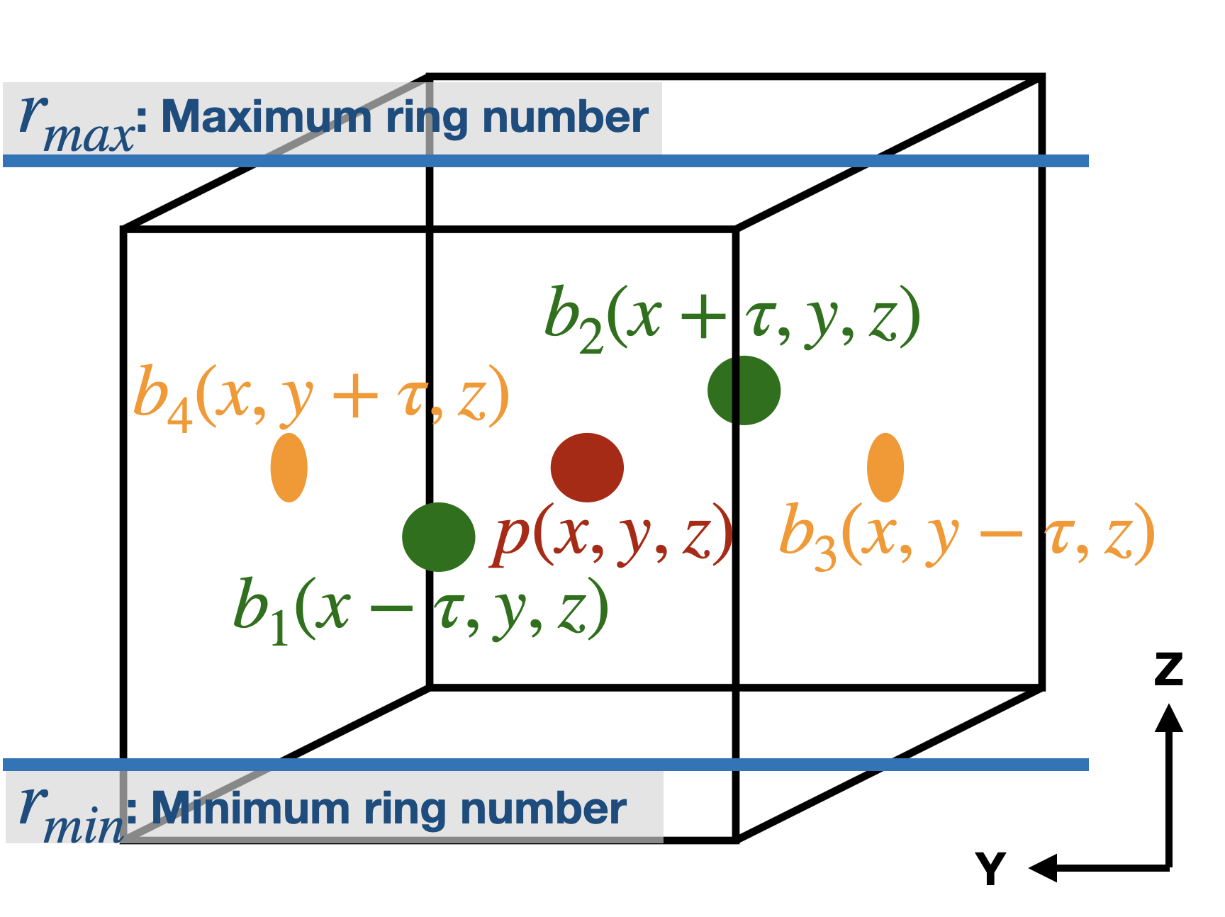
Figure 6: This figure shows the initial state of a cluster, in which has only single one feature. A cluster is defined as a cuboid in $\mathbb{R}^{3}$. When a feature fails at linkage, a cluster will be created and centered at itself $(x,y,z)$ with four boundaries $(x\pm\tau,y\pm\tau,z)$ for the $x$-$y$ axes, where $\tau$ is $t\sqrt{2}/4$, as well as the maximum ring number and the minimum ring number for the $z$-axis.

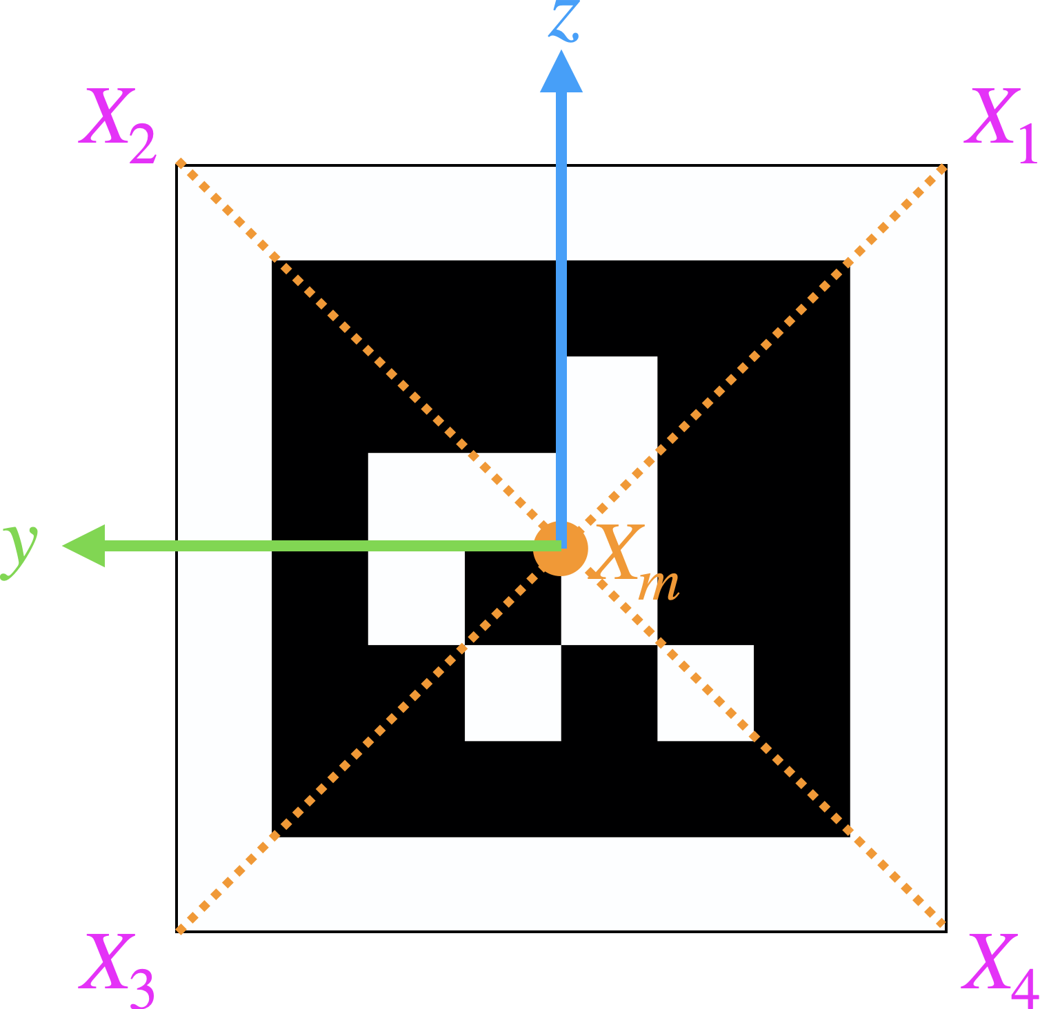
(a)

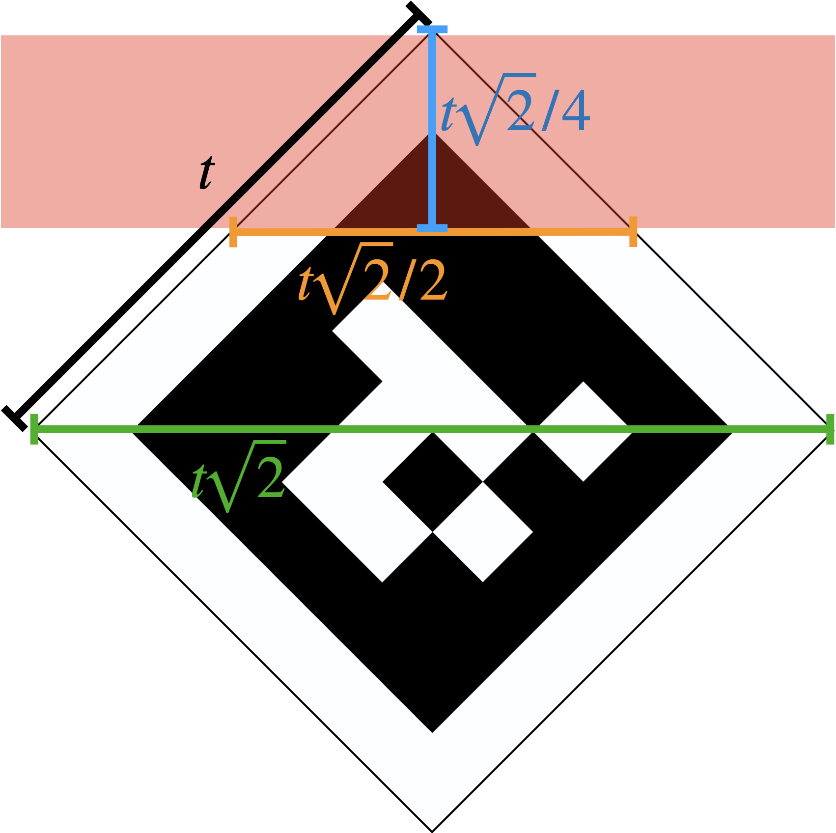
(b)

Figure 7: LABEL:sub@fig:PoseIllustration describes the coordinate system of the fiducial marker. LABEL:sub@fig:TopMostBeam indicates that the first beam hitting the LiDARTag should be at least $3/4$ above target, outlined as the red region.

IV-C Cluster Validation

At this point, we have grouped the features into clusters as shown in Fig 5a. In practice, few (possibly none) of the clusters will contain a valid tag and thus it is important to be able to eliminate clusters that are clearly invalid. To do so, we first used the point cloud data to fill in LiDAR returns between the features of a cluster, as shown in Fig. 5b.

Inspired by AprilTag [3, 4], tag-family-based heuristics are used to validate a cluster: number of points $\eta$ and number of features $\psi$ in the cluster. Another geometry-based heuristic is also deployed: the outlier percentage $(\kappa)$ of a plane fitting process. To save computation time, if any of the above processes fails, the cluster is marked as invalid and does not proceed to the next stage of validation. The first two values are determined by what type of tag family is chosen. Shown in Fig. 3c is a tag family which contains 16 bits.

A lower bound on the number of points in a cluster is determined by how many bits are contained in the fiducial marker. If the payload is $d\times d$, the LiDARTag including boundaries is $(d+4)\times(d+4)$. If we assume a minimum of five returns for each bit in the tag, then the minimum number points in a valid cluster is

$$\eta\geq 5(d+4)^{2}.$$ (3)

On the other hand, an upper bound is determined by the distance from the LiDAR to the marker and its size $t$. Given a tag at distance $D$, the maximum number of returns on the marker happens when it directly faces to the LiDAR and can be computed as:

$$M\frac{t\sqrt{2}}{D\sin{\theta}},$$ (4)

where $\theta$ is the horizontal resolution of the LiDAR, $M$ is the number of rings hitting on the tag, and $t\sqrt{2}$ is the diagonal length of the tag, as shown in Fig. 7b.

The boundaries of the payload can be detected by an intensity gradient,

$$\nabla I(p_{i,m})=|p_{i+\ell,m}^{I}-p_{i,m}^{I}|-|p_{i-\ell,m}^{I}-p_{i,m}^{I}|,$$ (5)

where $\ell$ is also a design choice (here, taken as one), and $p_{i,m}^{I}$ is the intensity value of the $i^{\text{th}}$ point on the $m^{\text{th}}$ ring. An example of detected boundary points is shown in Fig. 5c. If $\nabla I(p_{i,m})$ exceeds a threshold, then $p_{i,m}$ is a payload edge point. To successfully decode a tag, we will need at least one ring on each row of the payload. Hence, the minimum number of payload edge points is

$$\psi\geq 2(d+2).$$ (6)

Finally, we apply a plane fitting process to the remaining clusters. If the percentage of outliers of the plane fitting is more than $\kappa$ (chosen as $0.05$), the cluster is considered invalid.

The above heuristics allow us to extract a potential fiducial marker from the LiDARTag through features in both cluttered indoor and spacious outdoor environments. The next step is to estimate the pose of the marker.

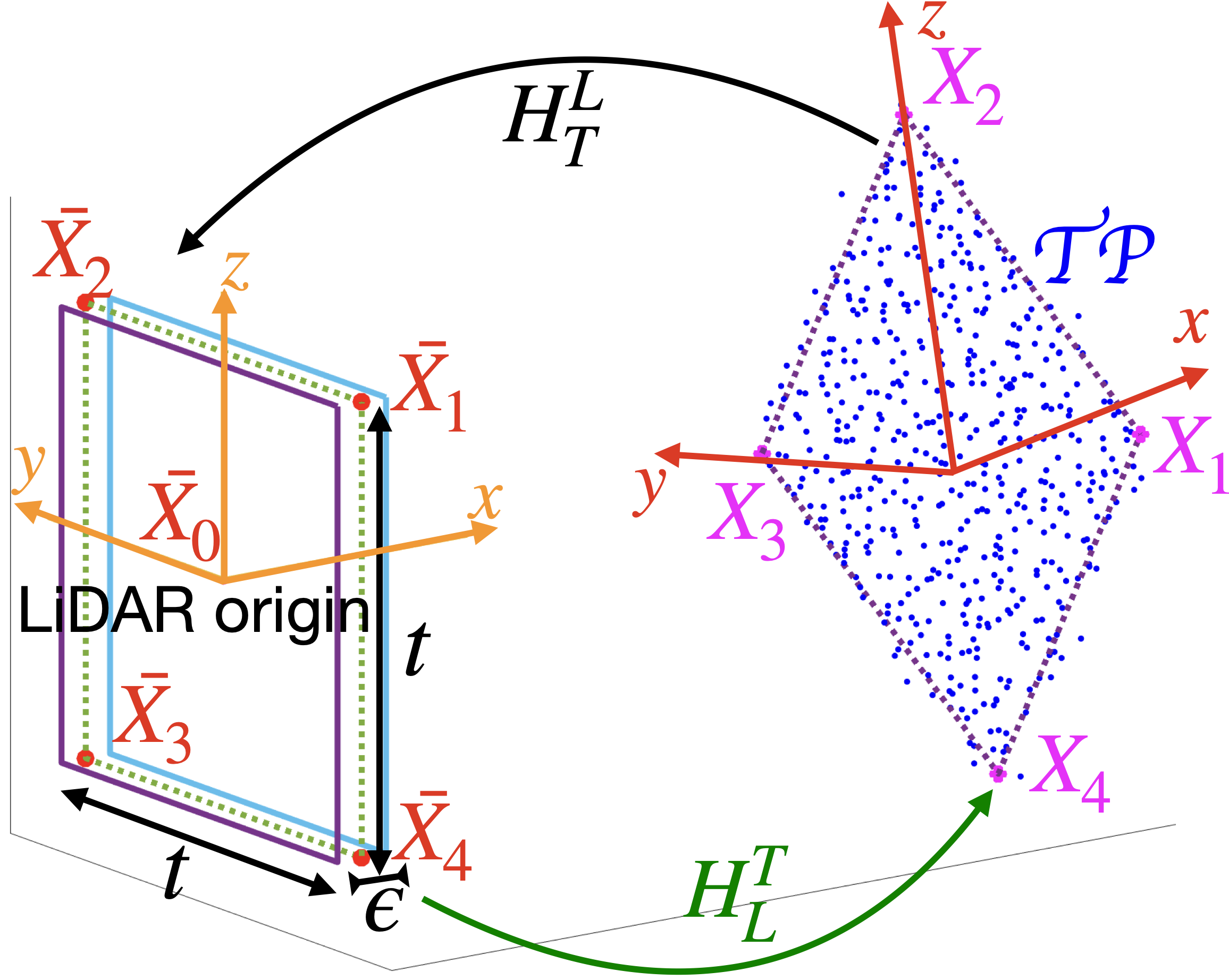
Figure 8: This conceptual figure illustrates the proposed method to estimate a LiDARTag’s pose. The target’s coordinate frame is defined as the mean of the four vertices $({X}_{1},\cdots,{X}_{4})$ and the template of known geometry is defined by $(\bar{X}_{1},\cdots,\bar{X}_{4})$ with depth $\epsilon$ at the LiDAR origin. The rigid-body transformation $H_{T}^{L}$ (black arrow) projects the target’s point cloud to the template. The actual pose of the LiDARTag is estimated by (9) using the inverse transformation $H_{T}^{L}$ (green arrow).

V Pose Estimation and Initialization

The pose of a LiDARTag is defined as $H_{L}^{T}$, a rigid-body transformation from the LiDAR frame to the LiDARTag frame, as shown in Fig. 8. To estimate the pose, we employ the $L_{1}$-inspired method proposed in [8]. The pose estimation is formulated into an optimization problem (9) in Sec. V-A. Due to $\mathrm{SE}(3)$ being non-convex and the requirement for a fast estimate, initial guesses to initialize the optimization problem and the gradient of the cost function are necessary, see Sec. V-B.

V-A LiDARTag Pose Estimation

Define the target point cloud $\mathcal{TP}:=\{\mathcal{X}_{i}\}_{i=1}^{M}$ as the collection of LiDAR returns from a LiDARTag, where $M$ is the number of points. Given the target geometry, we define a template with vertices $\{\bar{X}_{i}\}_{i=1}^{4}$ located at the origin of the LiDAR and aligned with the $y$-$z$ plane as defined in Fig. 8. We therefore seek a rigid-body transformation from LiDAR to the tag, $H_{L}^{T}\in\mathrm{SE}(3)$, that “best fits” the template onto the LiDAR returns of the target. In practice, it is actually easier to project the target point cloud $\mathcal{TP}$ back to the origin of the LiDAR through the inverse of the current estimate of transformation $H_{T}^{L}:=(H_{L}^{T})^{-1}$ and measure the error there. The action of $H\in\mathrm{SE}(3)$ on $\mathbb{R}^{3}$ is $H\cdot\mathcal{X}_{i}=R\mathcal{X}_{i}+p$, where $R\in\mathrm{SO}(3)$ and $p\in\mathbb{R}^{3}$. For $a\geq 0$ and $\lambda\in\mathbb{R}$, an $L_{1}$-inspired cost is defined as

$$c(\lambda,a):=\begin{cases}\min\{|\lambda-a|,|\lambda+a|\}&\text{if}~{}|\lambda|>a\\ 0&\text{otherwise}\end{cases}.$$ (7)

Let $\{\bar{\mathcal{X}}_{i}\}_{i=1}^{N}:=H_{T}^{L}(\mathcal{TP}):=\{H_{T}^{L}\cdot\mathcal{X}_{i}\}_{i=1}^{N}$ denote the projected point cloud by $H_{T}^{L}$, and denote a point’s $(x,y,z)$-entries by $(\bar{x}_{i},\bar{y}_{i},\bar{z}_{i})$. The total fitting error of the point cloud is defined as

$$C(H_{T}^{L}(\mathcal{TP})):=\sum_{i=1}^{M}c(\bar{x}_{i},\epsilon)+c(\bar{y}_{i},d/2)+c(\bar{z}_{i},d/2),$$ (8)

where $\epsilon\geq 0$ is a parameter to account for uncertainty in the depth measurement of the planar target and the principal axis with the smallest variance is used, see Sec. V-B. The optimization problem becomes

$$H_{T}^{L^{*}}:=\operatorname*{arg\,min}_{R_{T}^{L},p_{T}^{L}}C(H_{T}^{L}(\mathcal{TP})).$$ (9)

Finally, the pose of a LiDARTag is $H_{L}^{T}=H_{T}^{L^{*}};$ see [8] for more details. To solve this optimization problem, we leverage a gradient-based solver in the NLopt library [50] and the closed form of the gradient, which is provided on our GitHub [14].

Figure 5d shows the projected returns of a LiDARTag being inside the green box (aligned with the $y$-$z$ plane) at the LiDAR origin. In addition, we further compute the 2D convex hull within the $y$-$z$ plane of the pullback of point cloud and utilize the surveyor’s formula [51] to calculate the area of the convex hull. Our assumption on where first ring hits the marker results in at least 75% of the marker’s area being illuminated. Therefore, if the estimated area is less than 75% of the marker size, the cluster is considered invalid.

Remark 5.

Equation (9) provides an estimated rigid-body transformation from the LiDAR to the tag, and importantly, due to the symmetric of the target, the rotation of the tag about a normal vector to the tag may be off by $\pm 90^{\circ}$ or $180^{\circ}$. In particular, the four rotations in Fig. 9 are not determined. This ambiguity will be removed after decoding the tag, see Sec. VI.

V-B Optimization Initialization

The corners of the LiDARTags, $({X_{1}},\cdots,{X_{4}})$, are estimated from $\mathcal{TP}$. The initial guess of a rigid-body transformation is chosen to minimize the distance from the points $(\bar{X_{1}},\cdots,\bar{X_{4}})$ and $({X_{1}},\cdots,{X_{4}})$. This will be reduced to a (constrained orthogonal) procrustes problem [52], namely a problem of the form:

$$\Theta=\operatorname*{arg\,min}_{\begin{subarray}{c}\Omega:\ \Omega^{T}\Omega=I\end{subarray}}||\Omega A-B||_{F},$$ (10)

where for us, $\Omega$ will be a to-be-determined rotation matrix and $\lVert\cdot\rVert_{F}$ is the Frobenius norm.

Without loss of generality, $\bar{X_{0}}$ is assumed to be the origin, $(0,0,0)$ and ${X_{0}}$ is the mean of $\mathcal{TP}$. The translation $p$ is thus given by

$$\bar{X_{0}} =R{X_{0}}+p,\ \bar{X_{0}}=[0,0,0]^{\mathsf{T}}$$

$$p =-R{X_{0}}.$$ (11)

The rest of the problem can be formulated as:

$$\left\|H_{T}^{L}{X_{i}}-\bar{X_{i}}\right\|^{2}_{2} =\left\|\begin{bmatrix}R&p\\ \textbf{0}&1\end{bmatrix}\begin{bmatrix}{X_{i}}\\ 1\end{bmatrix}-\begin{bmatrix}\bar{X_{i}}\\ 1\end{bmatrix}\right\|_{2}^{2}$$ (12)

$$=\left\|R{X_{i}}+p-\bar{X_{i}}\right\|^{2}_{2}=\left\|R{X_{i}}^{\prime}-\bar{X_{i}}\right\|^{2}_{2},$$

$$\sum_{i=1}^{4}\left\|H_{T}^{L}{X_{i}}-\bar{X_{i}}\right\|^{2}_{2} =\sum_{i=1}^{4}\left\|R{X_{i}}^{\prime}-\bar{X_{i}}\right\|^{2}_{2}$$

$$=\left\|(R{X_{1}}^{\prime}-\bar{X_{1}})\vdots\ \cdots\ \vdots(R{X_{4}}^{\prime}-\bar{X_{4}})\right\|_{F}^{2}$$

$$=\left\|R{\textbf{X}}-\bar{\textbf{X}}\right\|^{2}_{F},$$ (13)

where ${X_{i}}^{\prime}={X_{i}}-{X_{0}}$, ${\textbf{X}}=\begin{bmatrix}{X_{1}}^{\prime}&{X_{2}}^{\prime}&{X_{3}}^{\prime}&{X_{4}}^{\prime}\end{bmatrix}$ and $\bar{\textbf{X}}=\begin{bmatrix}\bar{X_{1}}&\bar{X_{2}}&\bar{X_{3}}&\bar{X_{4}}\end{bmatrix}$. The problem is then

$$R^{\ast}=\operatorname*{arg\,min}_{\begin{subarray}{c}R:\ R^{T}R=I\end{subarray}}\left\|R{\textbf{X}}-\bar{\textbf{X}}\right\|_{F}^{2}.$$ (14)

By the procrustes optimization problem [52], we have a closed form solution:

$$M =\bar{\textbf{X}}{\textbf{X}}^{\mathsf{T}}=U\Sigma V^{\mathsf{T}}$$ (15)

$$R^{\ast} =UV^{\mathsf{T}}.$$ (16)

Remark 6.

To estimate X, we project the target point cloud $\mathcal{TP}$ along a principal axis of a Principal Components Analysis (PCA) [53]. Using the 2D projected point cloud, we use RANSAC to regress lines to determine target edges and solve for the intersections of the lines, to obtain an initialization of the vertices. The smallest variance of the principal axis is then used for the $\epsilon$ in (8). If the number of edge points is less than three, or any of edges fails when regressing a line, the cluster is marked as invalid.

(a)

(b)

(c)

(d)

Figure 9: Before decoding, the estimated rotation about the normal axis is only known modulo $90^{\circ}$, which means LABEL:sub@fig:codeword1 to LABEL:sub@fig:codeword4 yield the same normal vector. Accounting for the three possible rotations of $(\pm 90^{\circ},180^{\circ})$, results in 4 possible continuous functions in the function dictionary. When computing the inner product to the correct id of a LiDARTag, only one of the four functions is correct. From the correct function, the modulo $90^{\circ}$ ambiguity is removed.

VI Function Construction and Tag Decoding

In Sec. V-A, we defined a template at the LiDAR origin, estimated $H_{T}^{L}$, and we thus have the projected point cloud. Specifically, the projected point cloud is located at the LiDAR origin inside the template on the $y$-$z$ plane with the thickness being the sensor noise on the $x$-axis. Due to the sparsity of the point cloud, we construct a continuous function in an inner product space (RKHS) for the projected point cloud [9]. For each LiDARTag in the tag family, we pre-compute four continuous functions to account for four possible rotations, as shown in Fig. 9, consequently, resulting in a function dictionary. Each function is constructed by converting each pixel of the tag image to a point in $\mathbb{R}^{3}$, see [14] for implementation detail. Finally, we compute the inner product of the estimated function and each function in the dictionary. The largest inner product is the ID of the LiDARTag, and the ambiguity of rotation in Sec. V-A is removed.

Let $\mkern 1.5mu\widetilde{\mkern-1.5mu\mathcal{X}\mkern-1.5mu}\mkern 1.5mu:=\{(\mkern 1.5mu\widetilde{\mkern-1.5mup_{i}\mkern-1.5mu}\mkern 1.5mu,\ell(\mkern 1.5mu\widetilde{\mkern-1.5mup_{i}\mkern-1.5mu}\mkern 1.5mu))|\mkern 1.5mu\widetilde{\mkern-1.5mup_{i}\mkern-1.5mu}\mkern 1.5mu\in\mathbb{R}^{3}~{}\text{and}~{}\ell(\mkern 1.5mu\widetilde{\mkern-1.5mup_{i}\mkern-1.5mu}\mkern 1.5mu)\in\mathcal{I}\}_{i=1}^{M}$ be a collection of projected points, where $M$ is the number of points. In this work, we use the intensity as our information inner product space as $\mathcal{I}=\mathbb{R}$ and the inner product, $\langle\cdot,\cdot\rangle_{\mathcal{I}}$, is just the scalar product of intensity values. Therefore, the labels are simply the intensity values. The continuous function of $\mkern 1.5mu\widetilde{\mkern-1.5mu\mathcal{X}\mkern-1.5mu}\mkern 1.5mu$ is defined as

$$f(\cdot)=\sum_{i=1}^{M}\ell(\mkern 1.5mu\widetilde{\mkern-1.5mup_{i}\mkern-1.5mu}\mkern 1.5mu)k(\cdot,\mkern 1.5mu\widetilde{\mkern-1.5mup_{i}\mkern-1.5mu}\mkern 1.5mu),$$ (17)

where $k:\mathbb{R}^{3}\times\mathbb{R}^{3}\rightarrow\mathbb{R}$ is the kernel of an RKHS [9].

Given another continuous function $g$ of point cloud $\mkern 1.5mu\widetilde{\mkern-1.5mu\mathcal{Z}\mkern-1.5mu}\mkern 1.5mu:=\{(\mkern 1.5mu\widetilde{\mkern-1.5mup_{j}\mkern-1.5mu}\mkern 1.5mu,\ell(\mkern 1.5mu\widetilde{\mkern-1.5mup_{j}\mkern-1.5mu}\mkern 1.5mu))|\mkern 1.5mu\widetilde{\mkern-1.5mup_{j}\mkern-1.5mu}\mkern 1.5mu\in\mathbb{R}^{3}~{}\text{and}~{}\ell(\mkern 1.5mu\widetilde{\mkern-1.5mup_{j}\mkern-1.5mu}\mkern 1.5mu)\in\mathcal{I}\}_{j=1}^{N}$, where $N$ is the number of points. The inner product of $f$ and $g$ is

$$\langle f,g\rangle=\sum_{i=1}^{M}\sum_{j=1}^{N}\langle\ell(\mkern 1.5mu\widetilde{\mkern-1.5mup_{i}\mkern-1.5mu}\mkern 1.5mu),\ell(\mkern 1.5mu\widetilde{\mkern-1.5mup_{j}\mkern-1.5mu}\mkern 1.5mu)\rangle_{\mathcal{I}}k(\mkern 1.5mu\widetilde{\mkern-1.5mup_{i}\mkern-1.5mu}\mkern 1.5mu,\mkern 1.5mu\widetilde{\mkern-1.5mup_{j}\mkern-1.5mu}\mkern 1.5mu).$$ (18)

The kernel $k$ is modeled as the squared exponential kernel  [54, Chapter 4]:

$$k(\mkern 1.5mu\widetilde{\mkern-1.5mup_{i}\mkern-1.5mu}\mkern 1.5mu,\mkern 1.5mu\widetilde{\mkern-1.5mup_{j}\mkern-1.5mu}\mkern 1.5mu)=\sigma^{2}\text{exp}\left(-\frac{1}{2}(\mkern 1.5mu\widetilde{\mkern-1.5mup_{i}\mkern-1.5mu}\mkern 1.5mu-\mkern 1.5mu\widetilde{\mkern-1.5mup_{j}\mkern-1.5mu}\mkern 1.5mu)^{\mathsf{T}}\Lambda(\mkern 1.5mu\widetilde{\mkern-1.5mup_{i}\mkern-1.5mu}\mkern 1.5mu-\mkern 1.5mu\widetilde{\mkern-1.5mup_{j}\mkern-1.5mu}\mkern 1.5mu)\right),$$ (19)

where $\sigma^{2}$ is the signal variance (set to $1e5$) and $\Lambda$ is an isotropic diagonal length-scale matrix with its diagonal entry set to the inverse of squared half of the bit size of a LiDARTag: $1/(t/(2(d+4)))^{2}$. Let $t$ be the LiDARTag size, and the $d$-bit tag family is used ($d+4$ bits, including its boundaries). Then the bit size is $t/(d+4)$.

After applying the kernel trick to (18), we get [43]

$$\langle f,g\rangle=\sum_{i=1}^{M}\sum_{j=1}^{N}\,k_{\mathcal{I}}(\ell(\mkern 1.5mu\widetilde{\mkern-1.5mup_{i}\mkern-1.5mu}\mkern 1.5mu),\ell(\mkern 1.5mu\widetilde{\mkern-1.5mup_{j}\mkern-1.5mu}\mkern 1.5mu))\cdot k(\mkern 1.5mu\widetilde{\mkern-1.5mup_{i}\mkern-1.5mu}\mkern 1.5mu,\mkern 1.5mu\widetilde{\mkern-1.5mup_{j}\mkern-1.5mu}\mkern 1.5mu),$$ (20)

where

$$k_{\mathcal{I}}(\mkern 1.5mu\widetilde{\mkern-1.5mup_{i}\mkern-1.5mu}\mkern 1.5mu,\mkern 1.5mu\widetilde{\mkern-1.5mup_{j}\mkern-1.5mu}\mkern 1.5mu)=\text{exp}\left(-\frac{(\ell(\mkern 1.5mu\widetilde{\mkern-1.5mup_{i}\mkern-1.5mu}\mkern 1.5mu)-\ell(\mkern 1.5mu\widetilde{\mkern-1.5mup_{j}\mkern-1.5mu}\mkern 1.5mu))^{2}}{2l_{\mathcal{I}}^{2}}\right),$$ (21)

and the length-scale $l_{\mathcal{I}}$ is set to $10$ ($0\leq\ell(\mkern 1.5mu\widetilde{\mkern-1.5mup_{i}\mkern-1.5mu}\mkern 1.5mu)\leq 255$).

Remark 7.

To fully utilize the projected point cloud of LiDARTag returns, we extend the planar LiDARTag to a 3D LiDARTag based on the intensity value of each point in the point cloud. The linear transformation is defined as:

$$\mkern 1.5mu\widetilde{\mkern-1.5mup_{i}\mkern-1.5mu}\mkern 1.5mu=\begin{bmatrix}\mkern 1.5mu\widetilde{\mkern-1.5mux_{i}\mkern-1.5mu}\mkern 1.5mu\\ \mkern 1.5mu\widetilde{\mkern-1.5muy_{i}\mkern-1.5mu}\mkern 1.5mu\\ \mkern 1.5mu\widetilde{\mkern-1.5muz_{i}\mkern-1.5mu}\mkern 1.5mu\end{bmatrix}=\begin{bmatrix}1&0&0&\frac{t}{2(d+4)I_{max}}\\ 0&1&0&0\\ 0&0&1&0\end{bmatrix}\begin{bmatrix}\bar{x_{i}}\\ \bar{y_{i}}\\ \bar{z_{i}}\\ \bar{i_{i}}\end{bmatrix},$$ (22)

where $I_{max}$ is the maximum intensity of the point cloud and $t/(d+4)$ is the bit size.

Remark 8.

If the fitting error (8) in Sec. V-A is greater than $10\%$ of the number of points in the cluster or it is not able to decode the potential cluster in Sec. VI, this cluster is marked as invalid.

Remark 9.

Reproducing Kernel Hilbert Spaces have been widely used in the Representer Theorem [55, 56, 57] for various regularization problems, such as function estimation, classification and Support Vector Machines (SVM). These are typically high- or infinite-dimensional problems that while mathematically feasible, often appear to be not practically computable. With the help of RKHS and the Representer Theorem, the solutions to these problems can be formulated in lower-dimensional subspaces spanned by the “representers” of the data.

VII Experimental Results

We now present experimental evaluations of the proposed LiDARTag. In this work, we choose an easel as our 3D object to support the tag. Additionally, fiducial markers from the tag16h6 family of AprilTag3 are used, with sizes of 1.2, 0.8, 0.61 meters, as shown in Fig. 3. We do not compare the proposed LiDARTag system with camera-based tag systems because it is unfair to compare depth estimation from a LiDAR with depth estimation from a monocular camera. All experiments are conducted with a 32-Beam Velodyne ULTRA Puck LiDAR and an Intel RealSense camera rigidly attached to the torso of a Cassie-series bipedal robot as shown in Fig. 3d. We use the Robot Operating System (ROS) [13] to communicate and synchronize between sensors. The LiDARTag system runs faster than 100 Hz on a laptop equipped with Intel${}^{\text{\textregistered}}$ Core${}^{\text{TM}}$ i7-9750H CPU @ 2.60 GHz, which is similar to the processor on a robot coming to the market.

Datasets are collected in a cluttered laboratory to evaluate detection performance and a spacious outdoor facility, M-Air [58], equipped with a motion capture system to validate pose estimation and ID decoding. Additionally, false positives are evaluated on the Google Cartographer indoor dataset [11] and the outdoor Honda H3D datasets [12].

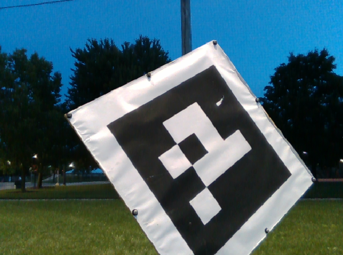
(a)

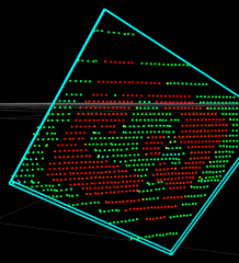
(b)

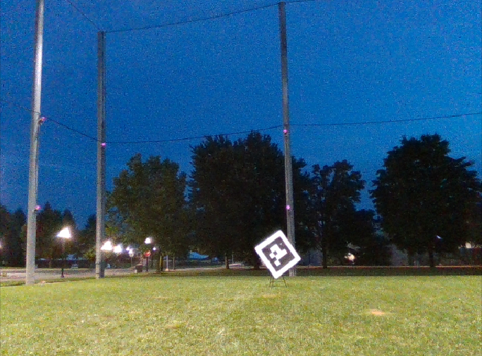
(c)

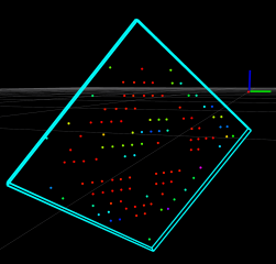
(d)

Figure 10: LABEL:sub@fig:MocapImgClose and LABEL:sub@fig:MocapImgFar are images of the tag placed at 2 and 14 meters away from a Cassie-series robot. LABEL:sub@fig:MocapTagClose and LABEL:sub@fig:MocapTagFar describe the results of projecting the template (green box) from the LiDAR origin to the tag’s returns by the poses of LiDARTag at 2 and 16 meters, respectively. While LABEL:sub@fig:MocapTagFar shows much sparser LiDAR returns than LABEL:sub@fig:MocapTagClose due to the farther distance, we are still able to accurately estimate the pose and its ID. Compared to ground truth provided by 30 motion capture cameras, the resulting poses are a few millimeters off in translation and a few degrees off in rotation.

TABLE I: Decoding accuracy of the RKHS method and pose accuracy of the fitting method. The ground truth is provided by a motion capture system with 30 motion capture cameras. The distance is in meters. The translation error is in millimeters and rotation error is the misalignment angle, (23), in degrees.

Face-on to LiDAR					Rotated at 45 degrees
Distance	No. Scans	No. Wrong ID	Translation Error	Rotation Error	Distance	No. Scans	No. Wrong ID	Translation Error	Rotation Error
2.15	73	0	14.03	0.44	2.13	74	0	0.27	0.05
4.29	72	0	10.13	0.67	3.95	134	0	0.52	0.34
5.90	81	0	16.23	0.44	5.93	137	0	0.36	0.05
7.97	78	0	1.32	0.21	7.92	126	0	0.26	0.32
10.12	87	0	1.64	0.40	10.38	130	0	4.91	1.03
12.14	69	0	2.07	0.36	12.12	71	0	5.78	0.39
13.87	35	1	2.81	10.48	14.08	49	2	1.98	15.92
Summary	No. Scans	Wrong ID Ratio	Translation Error	Rotation Error	Summary	No. Scans	Wrong ID Ratio	Translation Error	Rotation Error
mean	70	0.202 %	6.891	2.149	mean	103	0.276 %	1.744	2.586
std	16.88	–	6.418	4.577	std	37.25	–	2.076	5.888
median	73	–	2.81	0.44	median	126	–	0.52	0.34

VII-A Pose Evaluation and Decoding Accuracy

A motion capture system developed by Qualisys is used as a proxy for ground truth poses. The setup consists of 30 motion capture cameras with markers attached to tags, a LiDAR and a camera, as shown in Fig. 3d. Datasets are collected at various distances and angles. Each of the datasets contains images (20 Hz) and scans of point clouds (10 Hz). The 1.2-meter target is placed at distances from 2 to 14 meters in 2 meter increments. At each distance, data is collected with a target face-on to the LiDAR and another dataset with the target rotated by 45 degrees. More results and videos are on GitHub, see [14].

The optimization problem in (9) is solved with the method of moving asymptotes (MMA) algorithm [59, 60] provided in NLopt library [50]. We use the optimized LiDARTag pose to project the template at the LiDAR origin onto the LiDARTag’s returns to show the qualitative results of pose estimation. Figure 10b and Figure 10d show the pose of a tag at 2 meter and 16 meter, respectively. Even though the farther marker has much sparser LiDAR returns, by lifting the returns to an RKHS space, we are capable of correctly identifying its ID. In particular, a 1.2-meter target placed at 16 meters and rotated by 45 degrees is the detection limit of our 32-Beam Velodyne ULTRA Puck LiDAR. However, for a LiDAR with a different number of beams or points, the detection limit is subject to change. The more beams or points, the greater is the detection range. Using our LiDAR, the detectable angle is a little smaller than camera-based marker due to the sparse point clouds. Table I compares quantitatively the pose estimation between the proposed LiDARTag and ground truth. The translation error is reported in millimeters, and rotation error $\xi$ is represented as geodesic distance in degrees [61]:

$$\xi=\|\mathrm{Log}(\bar{R}\mkern 1.5mu\widetilde{\mkern-1.5muR\mkern-1.5mu}\mkern 1.5mu^{\mathsf{T}})\|,$$ (23)

where $\lVert\cdot\rVert$ is the Euclidean norm, $\bar{R}$ and $\mkern 1.5mu\widetilde{\mkern-1.5muR\mkern-1.5mu}\mkern 1.5mu$ are the ground truth and estimated rotation matrices, respectively, and $\mathrm{Log}(\cdot)$ is the logarithm map in the Lie group $\mathrm{SO}(3)$.

VII-B LiDARTag System and Speed Analysis

The computation time and cluster analysis of each step of the pipeline is shown in Table II. Indoors, we have fewer clusters because detected features are closer to each other resulting in many of them being clustered together. The computation time in an outdoor environment is faster than indoors because more clusters are rejected in the early stage due to the sparsity of the clusters, see Table  III. In both environments, the system achieves real-time performance (at least 100 Hz).

TABLE II: This table averages all the datasets we collected and describes computation time of each step for indoors and outdoors.

Outdoor
No. Points	No. Features	No. Clusters	Total Computation
51717	2179	271	114.86 Hz
PoI Clustering	Fill In Clusters	Point Check	Plane Fitting
2.63 ms	0.3 ms	0.00 ms	0.27 ms
Line Fitting	PCA	Pose Optimization	Tag Decoding
0.01 ms	0.03 ms	0.48 ms	3.34 ms
Indoor
No. Point Cloud	No. Features	No. Clusters	Total Computation
54277	1820	225	102.41 Hz
PoI Clustering	Fill In Clusters	Point Check	Plane Fitting
3.28 ms	0.22 ms	0.00 ms	0.15 ms
Line Fitting	PCA	Pose Optimization	Tag Decoding
0.01 ms	0.01 ms	0.42 ms	2.47 ms

TABLE III: This table takes into account all the data we collected and shows numbers of rejected clusters in each step in different scenes. Additionally, we also report false positive rejection for Cartographer and H3D dataset.

Outdoor
No. Min. Return	No. Max. Return	No. Plane Fitting
247.72	3.41	14.71
No. Boundary Points	No. Pose Estimation	No. Decoding Failure
4.10	0.48	0.00
Indoor
No. Min. Return	No. Max. Return	No. Plane Fitting
76.44	1.12	0.00
No. Boundary Points	No. Pose Estimation	No. Decoding Failure
8.14	1.80	1.16
Indoor Cartographer Dataset
No. Min. Return	No. Max. Return	No. Plane Fitting
65.76	0	1.90
No. Boundary Points	No. Pose Estimation	No. Decoding Failure
0.35	0	0
Outdoor H3D Dataset
No. Min. Return	No. Max. Return	No. Plane Fitting
713.35	8.72	44.41
No. Boundary Points	No. Pose Estimation	No. Decoding Failure
2.74	0.38	0

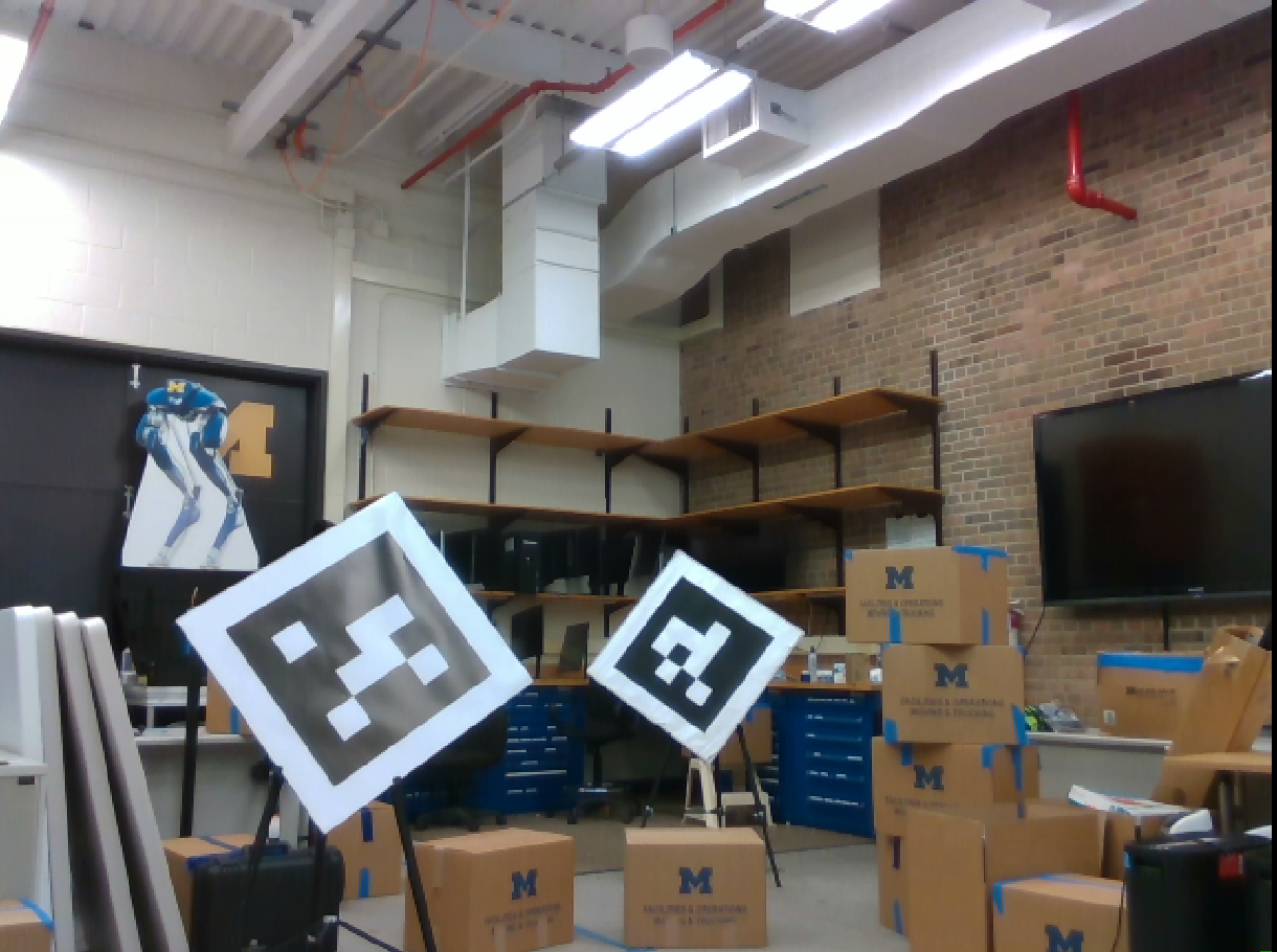
(a)

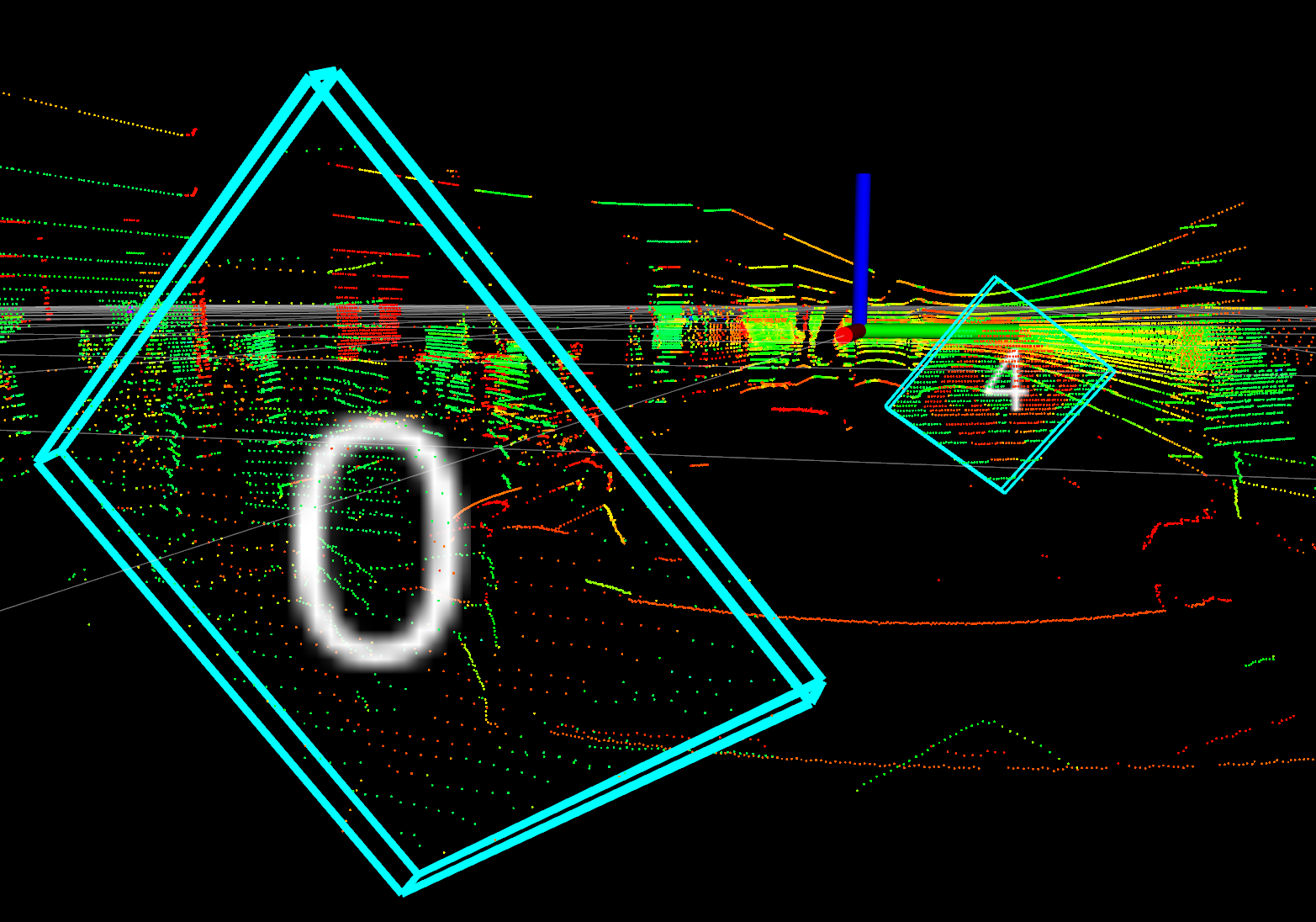
(b)

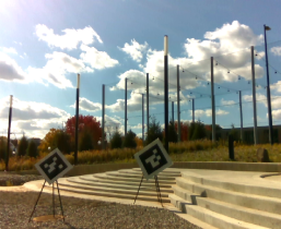
(c)

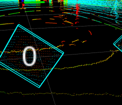
(d)

Figure 11: LABEL:sub@fig:TwoTagsLabImg and LABEL:sub@fig:TwoTagsOutsideImg image a 0.8 and a 0.6 meter tag placed in a cluttered indoor laboratory and a spacious outdoor environment. LABEL:sub@fig:TwoTagsInLabLiDAR and LABEL:sub@fig:TwoTagsOutsideLiDAR show the algorithm successfully detects the two markers of different sizes indicated by cyan boxes.

The original double sum in (18) takes over 140 milliseconds for each decoding process. To speed up the process, the inner sum of the double sum is transformed to a matrix and then to a vector form. For more details, see our implementation [14]. These two modifications boost the speed to 8.5 ms. However, this is still not fast enough because for each remaining cluster, (18) needs to be computed with all the tags in the function dictionary. Threading Building Blocks library (TBB) [62] is therefore used to further speed up this process to 2.4 ms. All together, the whole process was sped up by a factor of 60, from 144 ms to 2.4 ms. Furthermore, we also investigated the speed performance of employing a k-d tree data structure [63]. A summary Table IV is presented, showing that use of a k-d tree did not improve performance.

TABLE IV: The original double sum in (18) is too slow to achieve a real-time application. This table compares different methods to compute the double sum, in which the TBB stands for Threading Building Blocks library from Intel. Additionally, we also apply a k-d tree data structure to speed up the querying process; the k-d tree, however, does not produce fast enough results. The unit in the table is milliseconds.

Original Double Sum	Matrix Form	Vector From
144.18	67.11	8.51
TBB Original Form	TBB Vector Form	TBB k-d tree
35.68	2.40	5.73

VII-C False Positive Analysis

We have chosen some public datasets containing no ARTag features (i.e., no LiDARTags) so that there cannot be any false negatives and any detection of a LiDARTagin the datasets is consequently a false positive. To better verify the proposed LiDARTag algorithm, cluttered indoor scenes and crowded outdoor scenes are both necessary. The Google Cartographer indoor dataset [11] and Honda H3D outdoor dataset [12] were therefore used to validate the false positive rate of the proposed system. The Cartographer was collected with two Velodyne VLP-16 LiDARs in the Deutsches Museum. We took the longest three sequences consisting of more than 350 thousand LiDAR scans. Each scan contains about 30,000 points. We used the same algorithm with the same parameters and the full function dictionary that was used to detect the two tags in Fig. 11 (true positives were detected), and no false positives (i.e., no LiDARTags) were detected in the three sequences.

TABLE V: This table shows the numbers of false positive rejection of the proposed algorithm. We validated the rejection rate on the indoor Google Cartographer dataset and the outdoor Honda H3D datasets. The former has two VLP-16 Velodyne LiDAR and the latter has one 64-beam Velodyne LiDAR.

	Google Cartographer	Honda H3D
Scene	Indoor Museum	Crowed Driving Scenes
Duration	150 minutes	48 minutes
No. Scans	350 thousand	29 thousand
No. False Positives	0	0

The Honda H3D dataset was collected by a 64-beam Velodyne LiDAR and consists of 160 crowded and highly interactive traffic scenes in the San Francisco Bay Area. We evaluated on all sequences, resulting in 29 thousand LiDAR scans. Each scan consists of more than 130 thousand points. Zero targets were extracted by the detector. The results are shown in Table V. Additionally, false positives removed by each step are provided in Table III. Last but not the least, Fig. 11 shows that the detector is able to detect markers of different sizes both in a cluttered indoor scene and a spacious outdoor scene.

VIII Conclusion and Future Work

We presented a novel and flexible fiducial marker system specifically for point clouds. The developed fiducial tag system runs in real-time (faster than 100 Hz) while it can handle a full scan of raw point cloud from the employed 32-Beam Velodyne ULTRA Puck LiDAR (up to 120,000 points per scan). Each step of the proposed system was extensively analyzed and evaluated in both cluttered indoor as well as spacious outdoor environments. Furthermore, the system can be operated in a completely dark environment.

The LiDARTag pose estimation block deploys an $L_{1}$-inspired cost function. It achieved millimeter accuracy in translation and a few degrees of error in rotation compared to ground truth data collected by a motion capture system with 30 motion capture cameras. The sparse LiDAR returns on a LiDARTag are lifted to a continuous function in a reproducing kernel Hilbert space where the inner product is used to determine the marker’s ID, and this method achieved 99.7$\%$ accuracy. The rejection of false positives was evaluated on the Google Cartographer indoor dataset and the Honda H3D outdoor dataset. No false positives were detected in over 379 thousand LiDAR scans.

The presented fiducial marker system can also be used with cameras and has been successfully used for LiDAR-camera calibration in [8] and [10]. Additionally, the system is able to detect various marker sizes, whereas camera-based fiducial markers support one marker size at a time. In the future, we shall use the developed LiDARTag within SLAM systems to provide robot state estimation and loop closures. Because of different inherent properties of LiDARs and cameras, it would also be interesting to fuse a camera-based tag system and the proposed LiDARTag system. Currently, the proposed algorithm assumes the point cloud has been motion compensated; how to adopt motion distortion into the algorithm is an interesting direction for future work. Furthermore, if a dataset has been collected and labeled, a deep-learning architecture can replace the process of LiDARTag detection, thus offering another interesting area for future research.

References

- [1] D. Wagner and D. Schmalstieg, “Artoolkit on the pocketpc platform,” in IEEE International Augmented Reality Toolkit Workshop. IEEE, 2003, pp. 14–15.
- [2] M. Fiala, “Artag, a fiducial marker system using digital techniques,” in Proc. IEEE Conf. Comput. Vis. Pattern Recog., vol. 2. IEEE, 2005, pp. 590–596.
- [3] E. Olson, “AprilTag: A robust and flexible visual fiducial system,” in Proc. IEEE Int. Conf. Robot. and Automation. IEEE, 2011, pp. 3400–3407.
- [4] J. Wang and E. Olson, “Apriltag 2: Efficient and robust fiducial detection,” in Proc. IEEE/RSJ Int. Conf. Intell. Robots and Syst. IEEE, 2016, pp. 4193–4198.
- [5] M. Krogius, A. Haggenmiller, and E. Olson, “Flexible layouts for fiducial tags,” in Proc. IEEE/RSJ Int. Conf. Intell. Robots and Syst. IEEE, 2019, pp. 1898–1903.
- [6] J. DeGol, T. Bretl, and D. Hoiem, “Chromatag: a colored marker and fast detection algorithm,” in Proc. IEEE Conf. Comput. Vis. Pattern Recog., 2017, pp. 1472–1481.
- [7] ——, “Improved structure from motion using fiducial marker matching,” in Proc. European Conf. Comput. Vis., 2018, pp. 273–288.
- [8] J. Huang and J. W. Grizzle, “Improvements to target-based 3D LiDAR to camera calibration,” IEEE Access, vol. 8, pp. 134 101–134 110, 2020.
- [9] M. Ghaffari, W. Clark, A. Bloch, R. M. Eustice, and J. W. Grizzle, “Continuous direct sparse visual odometry from RGB-D images,” in Proc. Robot.: Sci. Syst. Conf., Freiburg, Germany, June 2019.
- [10] J.K. Huang and Jessy W. Grizzle, “Extrinsic LiDAR Camera Calibration,” 2019. [Online]. Available: https://github.com/UMich-BipedLab/extrinsic_lidar_camera_calibration
- [11] W. Hess, D. Kohler, H. Rapp, and D. Andor, “Real-time loop closure in 2D LIDAR SLAM,” in Proc. IEEE Int. Conf. Robot. and Automation. IEEE, 2016, pp. 1271–1278.
- [12] A. Patil, S. Malla, H. Gang, and Y.-T. Chen, “The H3D dataset for full-surround 3D multi-object detection and tracking in crowded urban scenes,” in Proc. IEEE Int. Conf. Robot. and Automation, 2019.
- [13] M. Quigley, K. Conley, B. Gerkey, J. Faust, T. Foote, J. Leibs, R. Wheeler, and A. Y. Ng, “ROS: an open-source Robot Operating System,” in ICRA workshop on open source software, 2009.
- [14] J.K. Huang and Jessy W. Grizzle, “LiDARTag: A Real-Time and Flexible Fiducial Tag for Point Clouds,” 2020. [Online]. Available: https://github.com/UMich-BipedLab/LiDARTag
- [15] M. Klopschitz and D. Schmalstieg, “Automatic reconstruction of wide-area fiducial marker models,” in Proc. Int. Symposium on Mixed and Augmented Reality. IEEE, 2007, pp. 71–74.
- [16] M. Velas, M. Spanel, Z. Materna, and A. Herout, “Calibration of RGB camera with velodyne LiDAR.” Václav Skala-UNION Agency, 2014.
- [17] Y. Park, S. Yun, C. S. Won, K. Cho, K. Um, and S. Sim, “Calibration between color camera and 3D LIDAR instruments with a polygonal planar board,” Sensors, vol. 14, no. 3, pp. 5333–5353, 2014.
- [18] B. Atcheson, F. Heide, and W. Heidrich, “Caltag: High precision fiducial markers for camera calibration.” in Vision, Modeling, and Visualization, vol. 10. Citeseer, 2010, pp. 41–48.
- [19] M. Fiala, “Comparing artag and artoolkit plus fiducial marker systems,” in Int. Workshop on Haptic Audio Visual Environments and their Applications. IEEE, 2005, pp. 6–pp.
- [20] A. Trachtenbert, “Computational methods in coding theory,” Master’s thesis, University of Illinois at Urbana-Champaign, 1996.
- [21] F. Bergamasco, A. Albarelli, E. Rodola, and A. Torsello, “Rune-tag: A high accuracy fiducial marker with strong occlusion resilience,” in Proc. IEEE Conf. Comput. Vis. Pattern Recog. IEEE, 2011, pp. 113–120.
- [22] L. Calvet, P. Gurdjos, C. Griwodz, and S. Gasparini, “Detection and accurate localization of circular fiducials under highly challenging conditions,” in Proc. IEEE Conf. Comput. Vis. Pattern Recog., 2016, pp. 562–570.
- [23] B. Wang, “LFTag: A scalable visual fiducial system with low spatial frequency,” arXiv preprint arXiv:2006.00842, 2020.
- [24] O. Grinchuk, V. Lebedev, and V. Lempitsky, “Learnable visual markers,” in Proc. Advances Neural Inform. Process. Syst. Conf., 2016, pp. 4143–4151.
- [25] D. Hu, D. DeTone, and T. Malisiewicz, “Deep charuco: Dark charuco marker pose estimation,” in Proc. IEEE Conf. Comput. Vis. Pattern Recog., 2019, pp. 8436–8444.
- [26] S. Song and J. Xiao, “Sliding shapes for 3d object detection in depth images,” in Proc. European Conf. Comput. Vis. Springer, 2014, pp. 634–651.
- [27] M. Engelcke, D. Rao, D. Z. Wang, C. H. Tong, and I. Posner, “Vote3deep: Fast object detection in 3D point clouds using efficient convolutional neural networks,” in Proc. IEEE Int. Conf. Robot. and Automation. IEEE, 2017, pp. 1355–1361.
- [28] S. Song and J. Xiao, “Voxelnet: End-to-end learning for point cloud based 3D object detection,” in Proc. IEEE Conf. Comput. Vis. Pattern Recog., 2018, pp. 4490–4499.
- [29] ——, “Deep sliding shapes for amodal 3D object detection in RGB-D images,” in Proc. IEEE Conf. Comput. Vis. Pattern Recog., 2016, pp. 808–816.
- [30] B. Li, “3D fully convolutional network for vehicle detection in point cloud,” in Proc. IEEE/RSJ Int. Conf. Intell. Robots and Syst. IEEE, 2017, pp. 1513–1518.
- [31] C. L. Zitnick and P. Dollár, “Edge boxes: Locating object proposals from edges,” in Proc. European Conf. Comput. Vis. Springer, 2014, pp. 391–405.
- [32] K. E. Van de Sande, J. R. Uijlings, T. Gevers, A. W. Smeulders, et al., “Segmentation as selective search for object recognition.” in Proc. IEEE Int. Conf. Comput. Vis., vol. 1, no. 2, 2011, p. 7.
- [33] J. Carreira and C. Sminchisescu, “Cpmc: Automatic object segmentation using constrained parametric min-cuts,” IEEE Trans. Pattern Anal. Mach. Intell., vol. 34, no. 7, pp. 1312–1328, 2011.
- [34] J. Li, S. Luo, Z. Zhu, H. Dai, A. S. Krylov, Y. Ding, and L. Shao, “3D IoU-Net: IoU guided 3D object detector for point clouds,” arXiv preprint arXiv:2004.04962, 2020.
- [35] S. Shi, X. Wang, and H. Li, “Pointrcnn: 3D object proposal generation and detection from point cloud,” in Proc. IEEE Conf. Comput. Vis. Pattern Recog., 2019, pp. 770–779.
- [36] A. Geiger, P. Lenz, C. Stiller, and R. Urtasun, “Vision meets robotics: The KITTI dataset,” Int. J. Robot. Res., 2013.
- [37] T. Hackel, N. Savinov, L. Ladicky, J. D. Wegner, K. Schindler, and M. Pollefeys, “SEMANTIC3D NET: A new large scale point cloud classification benchmark,” in ISPRS Annals of the Photogrammetry, Remote Sensing and Spatial Information Sciences, 2017, pp. 91–98.
- [38] W. Kim, M. S. Ramanagopal, C. Barto, M.-Y. Yu, K. Rosaen, N. Goumas, R. Vasudevan, and M. Johnson-Roberson, “Pedx: Benchmark dataset for metric 3-D pose estimation of pedestrians in complex urban intersections,” IEEE Robotics and Automation Letters, vol. 4, no. 2, pp. 1940–1947, 2019.
- [39] Velodyne Lidar, “Velodyne Ultra Puck: VLP-32C User Manual,” 2019. [Online]. Available: https://icave2.cse.buffalo.edu/resources/sensor-modeling/VLP32CManual.pdf
- [40] L. Naimark and E. Foxlin, “Circular data matrix fiducial system and robust image processing for a wearable vision-inertial self-tracker,” in Proc. Int. Symposium on Mixed and Augmented Reality. IEEE Computer Society, 2002, p. 27.
- [41] J. Rekimoto and Y. Ayatsuka, “Cybercode: designing augmented reality environments with visual tags,” in Proc. Designing augmented reality environments. ACM, 2000, pp. 1–10.
- [42] Y. Cho, J. Lee, and U. Neumann, “A multi-ring color fiducial system and an intensity-invariant detection method for scalable fiducial-tracking augmented reality,” in Proc. Int. Workshop on Augmented Reality. Citeseer, 1998.
- [43] W. Clark, M. Ghaffari, and A. Bloch, “Nonparametric continuous sensor registration,” arXiv preprint arXiv:2001.04286, 2020.
- [44] M. Ghaffari, W. Clark, A. Bloch, R. M. Eustice, and J. W. Grizzle, “Continuous direct sparse visual odometry from rgb-d images,” arXiv preprint arXiv:1904.02266, 2019.
- [45] J. Canny, “A computational approach to edge detection,” in Readings in computer vision. Elsevier, 1987, pp. 184–203.
- [46] T. Shan and B. Englot, “LeGO-LOAM: Lightweight and ground-optimized lidar odometry and mapping on variable terrain,” in Proc. IEEE/RSJ Int. Conf. Intell. Robots and Syst. IEEE, 2018, pp. 4758–4765.
- [47] S. C. Johnson, “Hierarchical clustering schemes,” Psychometrika, vol. 32, no. 3, pp. 241–254, 1967.
- [48] S. Lloyd, “Least squares quantization in PCM,” IEEE Trans. Inf. Theory, vol. 28, no. 2, pp. 129–137, 1982.
- [49] J. L. Bentley, “Multidimensional binary search trees used for associative searching,” Communications of the ACM, vol. 18, no. 9, pp. 509–517, 1975.
- [50] S. G. Johnson, “The nlopt nonlinear-optimization package,” 2014. [Online]. Available: https://github.com/stevengj/nlopt
- [51] B. Braden, “The surveyor’s area formula,” The College Mathematics Journal, vol. 17, no. 4, pp. 326–337, 1986.
- [52] J. C. Gower, “Generalized procrustes analysis,” Psychometrika, vol. 40, no. 1, pp. 33–51, 1975.
- [53] A. L. Price, N. J. Patterson, R. M. Plenge, M. E. Weinblatt, N. A. Shadick, and D. Reich, “Principal components analysis corrects for stratification in genome-wide association studies,” Nature genetics, vol. 38, no. 8, p. 904, 2006.
- [54] C. Rasmussen and C. Williams, Gaussian processes for machine learning. MIT press, 2006, vol. 1.
- [55] B. Schölkopf, R. Herbrich, and A. J. Smola, “A generalized representer theorem,” in Int. Conf. Computational Learning Theory. Springer, 2001, pp. 416–426.
- [56] G. Wahba, Spline models for observational data. SIAM, 1990.
- [57] G. Kimeldorf and G. Wahba, “Some results on Tchebycheffian spline functions,” vol. 33, no. 1, pp. 82–95, 1971.
- [58] “M-Air at the University of Michigan, Ann Arbor,” 2018. [Online]. Available: https://robotics.umich.edu/about/mair/
- [59] K. Svanberg, “A class of globally convergent optimization methods based on conservative convex separable approximations,” SIAM J. on optimization, vol. 12, no. 2, pp. 555–573, 2002.
- [60] ——, “The method of moving asymptotes: a new method for structural optimization,” Int. J. for numerical methods in engineering, vol. 24, no. 2, pp. 359–373, 1987.
- [61] D. Q. Huynh, “Metrics for 3D rotations: Comparison and analysis,” J. Math. Imaging and Vis., vol. 35, no. 2, pp. 155–164, 2009.
- [62] D. Padua, Ed., TBB (Intel Threading Building Blocks). Boston, MA: Springer US, 2011, pp. 2029–2029. [Online]. Available: https://doi.org/10.1007/978-0-387-09766-4_2080
- [63] J. L. Blanco and P. K. Rai, “nanoflann: a C++ header-only fork of FLANN, a library for nearest neighbor (NN) with kd-trees,” https://github.com/jlblancoc/nanoflann, 2014.