Extreme Events for Fractional Brownian Motion with Drift: Theory and Numerical Validation

Abstract

We study the first-passage time, the distribution of the maximum, and the absorption probability of fractional Brownian motion of Hurst parameter $H$ with both a linear and a non-linear drift. The latter appears naturally when applying non-linear variable transformations. Via a perturbative expansion in $\varepsilon=H-1/2$, we give the first-order corrections to the classical result for Brownian motion analytically. Using a recently introduced adaptive bisection algorithm, which is much more efficient than the standard Davies-Harte algorithm, we test our predictions for the first-passage time on grids of effective sizes up to $N_{\rm eff}=2^{28}\approx 2.7\times 10^{8}$ points. The agreement between theory and simulations is excellent, and by far exceeds in precision what can be obtained by scaling alone.

I Introduction

Understanding the extreme-value statistics of random processes is important in a variety of contexts. Examples are records MajumdarSchehrWergen2012 , e.g. in climate change WergenBognerKrug2011 , equivalent to depinning LeDoussalWiese2008a , in quantitative trading RejSeagerBouchaud2017 , or for earthquakes ShomeCornellBazzurroCarballo1998 . While much is known for Markov processes, and especially for Brownian motion RednerBook ; GumbelBook ; FellerBook ; FellerBook2 ; BorodinSalminen2002 ; BertoinBook ; Wiese2019 , much less is known for correlated, i.e. non-Markovian processes, of which fractional Brownian motion (fBm) is the simplest scale-free version NourdinBook ; Sottinen2001 ; Sinai1997 ; MandelbrotVanNess1968 ; Krug1998 ; DiekerPhD ; DiekerMandjes2003 ; Aurzada2011 .

FBm is important as it successfully models a variety of natural processes DecreusefondUstAOEnel1998 : a tagged particle in single-file diffusion ($H\,{=}\,0.25$) KrapivskyMallickSadhu2015 ; SadhuDerrida2015 , the integrated current in diffusive transport ($H\,{=}\,0.25$) SadhuDerrida2016 , polymer translocation through a narrow pore ($H\,{\simeq}\,0.4$) ZoiaRossoMajumdar2009 ; DubbeldamRostiashvili2011 ; PalyulinAlaNissilaMetzler2014 , anomalous diffusion BouchaudGeorges1990 , values of the log return of a stock ($H\,{\simeq}\,0.6\;{\rm to}\;0.8$) Peters1996 ; CutlandKoppWillinger1995 ; BiaginiHuOksendalZhang2008 ; Sottinen2001 , hydrology ($H\,{\simeq}\,0.72\;{\rm to}\;0.87$) MandelbrotWallis1968 , a tagged monomer in a polymer ($H\,{=}\,0.25$) GuptaRossoTexier2013 , solar flare activity ($H\,{\simeq}\,0.57\;{\rm to}\;0.86$) Monte-MorenoHernandez-Pajares2014 , the price of electricity in a liberated market ($H\,{\simeq}\,0.41$) Simonsen2003 , telecommunication networks ($H\,{\simeq}\,0.78\;{\rm to}\;0.86$) Norros2006 , telomeres inside the nucleus of human cells ($H\,{\simeq}\,0.18\;{\rm to}\;0.35$) BurneckiKeptenJanczuraBronshteinGariniWeron2012 , or diffusion inside crowded fluids ($H\,{\simeq}\,0.4$) ErnstHellmannKohlerWeiss2012 .

Recently, first-passage times of fBm have been investigated JeonChechkinMetzler2011 ; JeonChechkinMetzler2013 ; GuerinLevernierBenichouVoituriez2016 ; DelormeWiese2016 ; DelormeThesis ; DelormeWiese2015 . Due to the non-Markovian nature of the process, translating these results to a fBM with drift is far from trivial, and even properly estimating the drift for $H<1/2$ is a challenge Es-SebaiyOuassouOuknine2009 . To our knowledge, no anaytical result for a fBm with drift are known. It is this gap we intend to fill here.

As is discussed later, apart from a linear drift, a non-linear drift may appear as well, leading us to consider the process,

$$z_{t} := x_{t}+\mu t+\nu t^{2H}\ .$$ (1)

Here $x_{t}$ is a standard fractional Brownian motion (fBm) with mean and variance

$$\left<x_{t}\right> = x_{0}=0\ ,$$ (2)

$$\left<x_{t_{1}}x_{t_{2}}\right> = |t_{1}|^{2H}+|t_{2}|^{2H}-|t_{1}-t_{2}|^{2H}\ .$$ (3)

The parameter $H$ is the Hurst parameter. Since fBm is a Gaussian process, the above equations uniquely and completely specify it. Taking a derivative w.r.t. both $t_{1}$ and $t_{2}$ shows that the increments of the process are correlated,

$$\left<\dot{x}_{t_{1}}\dot{x}_{t_{2}}\right>=2H(2H-1)|t_{1}-t_{2}|^{2H-2}\ .$$ (4)

Correlations are positive for $H>1/2$, and negative for $H<1/2$. The case $H=1/2$ corresponds to Brownian motion, with uncorrelated increments.

The parameters $\mu$ and $\nu$ are the strength of linear and non-linear drift. While linear drift is a canonical choice, non-linear drift appears as a consequence of non-linear variable transformations. As an example, consider the process

$$y_{t}:=\mathrm{e}^{z_{t}}\ .$$ (5)

The exponential transformation appears quite often, be it in the Black-Sholes theory of the stock market where the logarithm of the portfolio price is treated as a random walk BlackScholes1973 ; CutlandKoppWillinger1995 ; BouchaudPotters2009 , be it in non-linear surface growth of the Kardar-Parisi-Zhang universality class KPZ ; Wiese1998a ; JanssenTauberFrey1999 , where the transformation is known as the Cole-Hopf transformation Hopf1950 ; Cole1951 , or in the evaluation of the Pickands constant DebickiKisowski2008 ; DelormeRossoWiese2017 ; HaanPickands1986 ; Harper2014 ; Michna2009 ; Pickands1969 ; Pickands1971 ; Pickands1975 . Like any non-linear transform, this generates an effective drift known from Itô-calculus. Computing the average of $y_{t}$ gives

$$\left<y_{t}\right> = \left<\mathrm{e}^{z_{t}}\right>=\exp\!\left({\left<z_{t}\right>+\frac{1}{2}\left[\left<z_{t}^{2}\right>-\left<z_{t}\right>^{2}\right]}\right)$$ (6)

$$= \exp\!\Big{(}\mu t+\left[\nu+1\right]t^{{2H}}\Big{)}\ .$$

Thus even if initially there is no nonlinear drift, it is generated by non-linear transformations. For this reason, we include it into our model.

While for Brownian motion, equivalent to $H=\frac{1}{2}$, many results can be obtained analytically RednerBook ; GumbelBook ; FellerBook ; FellerBook2 ; BorodinSalminen2002 ; BertoinBook ; Wiese2019 , for fBm much less is known. Recently, some of us developed a framework WieseMajumdarRosso2010 for a systematic expansion in

$$\varepsilon:=H-\frac{1}{2}\ .$$ (7)

It has since successfully been applied to obtain the distribution of the maximum and minimum of an fBm DelormeWiese2015 ; DelormeWiese2016 , to fBm bridges DelormeWiese2016b , evaluation of the Pickands constant DelormeRossoWiese2017 , the 2-sided exit problem Wiese2018 and the generalization of the three classical arcsine laws SadhuDelormeWiese2017 . It is also known that the fractal dimension of the record set of an fBm is $d_{\rm f}=H$ BenigniCoscoShapiraWiese2017 .

This article is organized into four sections, the introduction, theory in section II, and numerics in section 5, followed by conclusions in section IV.

P	probability
$~{}~{}P=\partial_{x}\bf P~{}~{}$	probability density in $x$
$~{}~{}\mathbb{P}=\partial_{t}\bf P~{}~{}$	probability density in $t$
$~{}~{}\mathcal{P}=\partial_{y}\bf P~{}~{}$	probability density in $y$

Table 1: Notations used for probabilities and their various densities.

II Theory

In this section, we find the probability distribution of first-passage times and running maxima of fBm with linear and non-linear drift by way of a perturbation expansion around simple Brownian motion. The key result of this section is the scaling function (II.12) which together with the auxiliary functions defined in Eqs. (II.12), (103) and (107) gives the distribution of first-passage times. The majority of this section is devoted to deriving these results.

II.1 Scaling dimensions

Before developing the perturbation theory, we consider the scaling dimensions involved. This will be useful for later discussion of the scaling functions. For fBm as defined in Eq. (1), there are four dimension-full quantities, $x$, $t$, $\mu$, and $\nu$. Scaling functions will thus depend on three scaling variables, which we now identify. We start with the terms without drift:

$$x\sim t^{H}~{}~{}\Longleftrightarrow~{}~{}t\sim x^{\frac{1}{H}}\ ,$$ (8)

where the tilde means “same scaling dimension”. Thus (without drift), any observable $\mathfrak{O}(x,t)$ can be written as

$$\mathfrak{O}(x,t)=x^{{\rm dim}_{x}({\mathfrak{O}})}f_{\mathfrak{O}}(y)\ ,\qquad y:=\frac{x}{\sqrt{2}t^{H}}\ .$$ (9)

The variable $y$ is dimension free. In presence of a linear drift, one has

$$x\sim\mu t~{}~{}\Longleftrightarrow~{}~{}\mu\sim\frac{x}{t}\sim x^{1-\frac{1}{H}}\sim t^{H-1}\ .$$ (10)

Thus the combination $u=\mu x^{\frac{1}{H}-1}$ is dimension free, as is $\tilde{u}:=u^{\frac{H}{1-H}}=\mu^{{\frac{H}{1-H}}}x$. For non-linear drift, we have

$$x\sim\nu t^{2H}~{}~{}\Longleftrightarrow~{}~{}\nu\sim\frac{x}{t^{2H}}\sim\frac{1}{x}\sim\frac{1}{t^{H}}\ .$$ (11)

Another scaling variable therefore is $v=\nu x.$ In conclusion, any observable $\mathcal{O}$ can, in generalization of Eq. (9), be written as

$$\mathfrak{O}(x,t,\mu,\nu) = x^{{\rm dim}_{x}({\mathfrak{O}})}f_{\mathfrak{O}}(y,u,v)\ ,$$ (12)

$$y = \frac{x}{\sqrt{2}t^{H}}\ ,$$ (13)

$$u=\mu x^{\frac{1}{H}-1}, \mbox{or\quad}\tilde{u}=\mu^{{\frac{H}{1-H}}}x\ ,$$ (14)

$$v = \nu x\ .$$ (15)

II.2 The first-passage time

The central result of our work is a perturbative expression of the first-passage-time density of fBM with linear and nonlinear drift as introduced in Eq. (1). The first-passage time $t_{\rm FP}$ is defined as

$$t_{\rm FP}(m):=\inf_{t>0}\left\{t,z_{t}\leq 0|z_{t=0}=m\right\}\ ,$$ (16)

where $m$ is the starting point of the process $z_{t}$, and $m>0$. The first-passage-time density for Brownian motion with (linear) drift, see e.g. RednerBook , and rederived below in Eq. (30), is

$$\mathbb{P}_{0}(t_{\rm FP}(m)=t)=\frac{m}{2\sqrt{\pi}t^{3/2}}\mathrm{e}^{-\frac{1}{2}\!\big{(}\frac{m}{\sqrt{2t}}+\frac{\mu}{2}\sqrt{2t}\big{)}^{2}}\ .$$ (17)

This density in time is most naturally expressed in terms of the scaling variable $y$ introduced in Eq. (9), and which for Brownian motion ($H=1/2$) reads

$$y=\frac{m}{\sqrt{2t}}\bigg{|}_{t=t_{\rm FP}(m)}\ .$$ (18)

For Brownian Motion the probability distribution of $y$ takes the simple form

$$\mathcal{P}_{0}(y;\mu) =\sqrt{\frac{2}{\pi}}\,\mathrm{e}^{-{\mathcal{F}}_{0}(y;\mu)}\ ,$$ (19)

$${\mathcal{F}}_{0}(y;\mu) =\frac{1}{2}\left(y+\frac{\mu}{2}\frac{m}{y}\right)^{2}\ .$$ (20)

Note that the measure is $\mathrm{d}t$ in Eq. (17) (density in time), whereas in Eq. (19) it is $\mathrm{d}y$ (density in $y$). To avoid confusion, we use distinct symbols for probabilities $\mathbf{P}$, densities $\mathbb{P}$ in time $t$, densities $\cal P$ in $y$, and densities $P$ in space $x$, independent of the actual choice of variables. This is summarized in table 1.

We introduced the scaling function ${\mathcal{F}}_{0}$. Below we compute its corrections to first order in $\varepsilon$, leading to a correction of the first-passage density in $y$,

$${\mathcal{P}(y;\mu,\nu)}=\frac{y^{\frac{1}{H}-2}}{\sqrt{2\pi}}\mathrm{e}^{-{\mathcal{F}}_{0}(y;\mu,\nu)-\varepsilon\delta{\mathcal{F}}(y;\mu,\nu)}+\mathcal{O}(\varepsilon^{2})\ .$$ (21)

The result is given in Eqs. (92)-(II.12). Two comments are in order: (i) the exponential resummation is chosen for better convergence for larger $\varepsilon$, as discussed in Wiese2018 , section IV.C; (ii) the distribution of first-passage times is related to the distribution of maxima.

Readers wishing to skip ahead will find the function $\delta{\mathcal{F}}$ evaluated using path-integral methods, described in section II.5. For the explicit result, see section II.12. A confirmation by numerical simulations is shown in section III.2.

II.3 Summary of calculations to be done

In order to calculate the first-passage-time distribution, we consider the process $z_{t}>0$ in the presence of an absorbing boundary condition at $z=0$ and restrict ourselves to $z_{t}>0$. The transition probability density of the process $z_{t}$ to pass from $z_{0}>0$ to $z_{1}>0$ in time $t$, without being absorbed at $z=0$ is denoted $P_{+}^{\mu,\nu}(z_{0},z_{1};t)$. The probability density of first-passage times $\mathbb{P}\big{(}t_{\rm FP}(m)=t\big{)}$ can then be obtained as

$$\mathbb{P}(t_{\rm FP}(m)=t)=\left.\partial_{z_{1}}P_{+}^{\mu,\nu}(m,z_{1},t)\right|_{z_{1}=0}.$$ (22)

This relation holds since the derivative on the right-hand-side picks out those trajectories which assume $z_{t}=0$ at time $t$ for the first time. The general strategy of this work is to compute $\left.\partial_{z_{1}}P_{+}^{\mu,\nu}(m,z_{1},t)\right|_{z_{1}=0}$ and its perturbative corrections using path-integral methods. In the subsequent section II.4, we discuss the reference point of our expansion, simple Brownian motion. In section II.5, we introduce a perturbative expansion around Brownian motion, based on a path-integral formalism. This yields a diagrammatic expansion (section II.6), with three diagrams, listed in section II.7, evaluated in sections II.8 to II.10, and regrouped in section II.11. The final result is given in section II.12. Contrary to the drift-free case, not all processes are absorbed, as is discussed in section II.13. Relations between the different probability densities are discussed in section II.14, followed by an analysis of the tail of these distributions in section II.15. Numerical checks are presented in section 5, followed by conclusions in section IV.

II.4 Simple Brownian Motion: First-passage time and absorption probability

The perturbation theory is an expansion around simple Brownian motion. This base point is considered here. By setting $H=\frac{1}{2}$ and $\nu=0$ in Eq. (1), we obtain simple Brownian motion with drift. For this process, we compute (i) the positive transition probability and (ii) the absorption probability.

The transition probability of simple Brownian motion $P_{+}^{\mu}$ (to alleviate our notations, we do not put an index $0$ to indicate Brownian motion, since $P_{+}$ is not used for fBm), the probability to pass from $z_{0}$ to $z_{1}$ within time $t$ without crossing the line $z\equiv 0$, satisfies the associated Fokker-Planck equation

$$\partial_{t}P_{+}^{\mu}(z_{0},z_{1},t)=\partial_{z_{1}}^{2}P_{+}^{\mu}(z_{0},z_{1},t)-\mu\partial_{z_{1}}P_{+}^{\mu}(z_{0},z_{1},t)\ .$$ (23)

with appropriate absorbing boundary condition at $z\equiv 0$. Its solution is given by the mirror-charge solution

$$P_{+}^{\mu}(z_{0},z_{1},t) = \frac{1}{\sqrt{4\pi t}}\left(\mathrm{e}^{-(z_{1}-z_{0})^{2}/4t}-\mathrm{e}^{-(z_{1}+z_{0})^{2}/4t}\right)$$ (24)

$$\times\mathrm{e}^{\frac{\mu}{2}(z_{1}-z_{0})-\frac{\mu^{2}t}{4}}\ ,$$

satisfying the initial condition

$$P_{+}^{\mu}(z_{0},z_{1},t=0)=\delta(z_{0}-z_{1})\ .$$ (25)

It is useful to consider its Laplace-transformed version. We define the Laplace transform of a function $f(t)$, with $t\geq 0$ as

$$\tilde{f}(s):=\mathcal{L}_{t\to s}\left[f(t)\right]=\int_{0}^{\infty}\mathrm{d}t\,\mathrm{e}^{-st}f(t)\ .$$ (26)

This yields

$$\tilde{P}_{+}^{\mu}(z_{0},z_{1},s)=\mathrm{e}^{\frac{\mu}{2}(z_{1}-z_{0})}\tilde{P}_{+}\Big{(}z_{0},z_{1},s+\frac{\mu^{2}}{4}\Big{)}\ ,$$ (27)

where the drift-free propagator reads

$$\tilde{P}_{+}(z_{0},z_{1},s)=\frac{\mathrm{e}^{-\sqrt{s}\left(z_{0}-z_{1}\right)}-\mathrm{e}^{-\sqrt{s}\left(z_{0}+z_{1}\right)}}{2\sqrt{{s}}}\ .$$ (28)

The Laplace transform $\tilde{\mathbb{P}}(m,s)$ of the first-passage-time probability density, following Eq. (22), equals the probability to go close to the boundary, and there being absorbed for the first time,

$$\tilde{\mathbb{P}}(m,s) :=\int_{0}^{\infty}{\rm d}t\,e^{-st}{\mathbb{P}}(t_{\rm FP}(m)=t)$$

$$=\left.\partial_{z_{1}}\tilde{P}_{+}^{\mu}(m,z_{1},s)\right|_{z_{1}=0}$$

$$=\mathrm{e}^{-\frac{\mu}{2}m}\mathrm{e}^{-m\sqrt{s+\mu^{2}/4}}\ .$$ (29)

Its inverse Laplace transform is the first-passage-time probability density

$$\mathbb{P}(t_{\rm FP}(m)=t) = \mathrm{e}^{-\frac{\mu}{2}m-\frac{\mu^{2}}{4}t}\frac{m\mathrm{e}^{-\frac{m^{2}}{4t}}}{2\sqrt{\pi}t^{3/2}}\ ,$$ (30)

confirming the result in Eq. (17). The total (time integrated) absorption probability is

$$\mathbf{P}_{\rm abs}(m) = \tilde{\mathbb{P}}(m,s=0)$$ (33)

$$= \mathrm{e}^{-\frac{\mu}{2}m}\mathrm{e}^{-\frac{|\mu|}{2}m}=\left\{\begin{array}[]{ccc}\mathrm{e}^{-\mu m}&,&~{}\mu>0\\ 1&,&~{}\mu\leq 0\end{array}\right.\ .\qquad$$

In what follows, we present perturbative corrections of these results for $\varepsilon\neq 0$.

II.5 The path-integral of a fBm with drift

The technology developed in WieseMajumdarRosso2010 ; DelormeWiese2016 ; Wiese2018 uses a path-integral to describe fBM. Since $z_{t}$ is Gaussian, its path-probability measure on a finite interval $[0,T]$ is

$${\bf P}[z_{t}]=\exp\left(-\mathcal{S}[z_{t};\mu,\nu]\right)\ ,$$ (34)

where $\mathcal{S}[z_{t};\mu,\nu]$ is an action quadratic in $z_{t}$. Without drift ($\mu=\nu=0$), the action for a fBM to order $\varepsilon$ is WieseMajumdarRosso2010 ; DelormeWiese2016 ; Wiese2018

$$\mathcal{S}[z_{t};\mu=\nu=0]$$ (35)

$$=\int_{0}^{T}\mathrm{d}t\,\frac{\dot{z}_{t}^{2}}{4D_{\varepsilon}}-\frac{\varepsilon}{2}\int_{\tau}^{T}\mathrm{d}t_{2}\int_{0}^{t_{2}-\tau}\mathrm{d}t_{1}\frac{\dot{z}_{t_{1}}\dot{z}_{t_{2}}}{|t_{1}-t_{2}|}\ .$$

The action consists of a local part, corresponding to simple Brownian motion, and a non-local part, proportional to $\varepsilon$. The idea behind the perturbative expansion is that Brownian motion (as given by the first term) samples the whole phase space of fBm, albeit with the wrong probability measure. Our perturbation theory corrects this, by weighing each path with the second term in Eq. (35). This implies that the absorbing boundary conditions at the origin are properly taken into account, and that observables as the absorption current, which are given by local operators, remain valid. For regularity, a short-distance cutoff $|t_{1}-t_{2}|>\tau$ is introduced in the last integral, which is reflected in the diffusion constant DelormeWiese2016

$$D_{\varepsilon}=2H\tau^{2H-1}=(1+2\varepsilon)\tau^{2\varepsilon}=(\mathrm{e}\tau)^{2\varepsilon}+\mathcal{O}(\varepsilon^{2})\ .$$ (36)

Let us now insert the definition (1) into the action (35). The reason to proceed this way is that the method of images on which our further calculation relies works in terms of $x_{t}$ as defined in Eq. (1), but not $z_{t}$. After some algebra we arrive at the action for an arbitrary drift

$${\cal S}[z_{t}] = \int_{0}^{T}\mathrm{d}t\,\frac{\dot{z}_{t}^{2}}{4D_{\varepsilon}}$$ (37)

$$+\int_{0}^{T}\mathrm{d}t\frac{\varepsilon}{2}\dot{z}_{t}\left[(\mu{+}\nu)\ln\left(\frac{t(T{-}t)}{\tau^{2}}\right)-2\nu\ln\left(\frac{t}{\tau}\right)\right]$$

$$-\frac{\varepsilon}{2}\int_{\tau}^{T}\mathrm{d}t_{2}\int_{0}^{t_{2}-\tau}\mathrm{d}t_{1}\frac{\dot{z}_{t_{1}}\dot{z}_{t_{2}}}{|t_{1}-t_{2}|}$$

$$-\frac{z_{T}-z_{0}}{2}\Big{[}{\frac{\mu}{D_{\varepsilon}}+\nu}\Big{]}+\frac{T}{4}(\mu+\nu)^{2}$$

$$+\frac{T}{2}\varepsilon\left(\nu^{2}-\mu^{2}\right)\ln(T)+\ {\cal O}(\varepsilon^{2})\ .$$

Some checks are in order. In absence of absorbing boundaries, the exact free propagator reads

$$\!\!P^{\mu,\nu}(0,z,T) = \frac{1}{2\sqrt{\pi}T^{H}}\mathrm{e}^{-\frac{(z-\mu T-\nu T^{2H})^{2}}{4T^{2H}}}$$ (38)

$$= \frac{1}{2\sqrt{\pi}T^{H}}\exp\bigg{(}{-}\frac{z^{2}}{4T^{2H}}+\frac{z}{2}\Big{[}\nu{+}\mu T^{-2\varepsilon}\Big{]}$$

$$~{}~{}~{}~{}~{}~{}~{}~{}~{}~{}~{}~{}~{}~{}~{}~{}~{}~{}~{}~{}~{}~{}~{}~{}~{}{-}\frac{T}{4}\Big{[}\nu T^{\varepsilon}{+}\mu T^{-\varepsilon}\Big{]}^{2}\bigg{)}.~{}~{}~{}~{}~{}~{}~{}$$

Since the above formalism has variables $\dot{z}$ only, the term $\sim z^{2}$ is given by the drift-free perturbation theory. We can further check that if we replace in the action $\dot{z}(t)$ by its “classical trajectory”, i.e. $\dot{z}(t)\to[z(T)-z(0)]/T$, then both the normalization and the drift term agree with the exact propagator.

Let us specify Eq. (37) to the two cases of interest: For a fBm with linear drift as given in Eq. (1) with $\nu=0$, we have

$${\cal S}_{\nu=0}[z_{t}] = \int_{0}^{T}\mathrm{d}t\,\frac{\dot{z}_{t}^{2}}{4D_{\varepsilon}}-\frac{\mu}{2D_{\varepsilon}}(z_{T}-z_{0})+\frac{T^{1-2\varepsilon}}{4}\mu^{2}$$ (39)

$$-\frac{\varepsilon}{2}\int_{\tau}^{T}\mathrm{d}t_{2}\int_{0}^{t_{2}-\tau}\mathrm{d}t_{1}\frac{\dot{z}_{t_{1}}\dot{z}_{t_{2}}}{|t_{1}-t_{2}|}$$

$$+\frac{\varepsilon\mu}{2}\int_{0}^{T}\mathrm{d}t\,\dot{z}_{t}\ln\left(\frac{[T-t]t}{\tau^{2}}\right)+\mathcal{O}(\varepsilon^{2})\ .~{}~{}~{}~{}~{}~{}~{}$$

For a fBm with non-linear drift as given in Eq. (1) with $\mu=0$, we have

$${\cal S}_{\mu=0}[z] = \int_{0}^{T}\mathrm{d}t\,\frac{\dot{z}_{t}^{2}}{4D_{\varepsilon}}-\frac{\nu}{2}(z_{T}-z_{0})+\frac{T^{1+2\varepsilon}}{4}\nu^{2}$$ (40)

$$-\frac{\varepsilon}{2}\int_{\tau}^{T}\mathrm{d}t_{2}\int_{0}^{t_{2}-\tau}\mathrm{d}t_{1}\frac{\dot{z}_{t_{1}}\dot{z}_{t_{2}}}{|t_{1}-t_{2}|}$$

$$+\frac{\varepsilon\nu}{2}\int_{0}^{T}\mathrm{d}t\,\dot{z}_{t}\ln\left(\frac{T-t}{t}\right)+\mathcal{O}(\varepsilon^{2})\ .~{}~{}~{}~{}~{}~{}~{}$$

Note the appearance of the diffusion constant in the “bias” (Girsanov) term $z_{T}-z_{0}$ for a linear drift, and its absence for a non-linear drift.

To simplify the notation, we introduce

$$\mathcal{S}_{0}[z_{t}]=\int_{0}^{T}\mathrm{d}t\,\frac{\dot{z}_{t}^{2}}{4}$$ (41)

as a shorthand for the Brownian action around which perturbation theory expands. The drift (Girsanov) term is $\mathrm{e}^{-\mathcal{S}_{\rm d}}$, with

$$\mathcal{S}_{\rm d}[z]=\frac{z_{0}-z_{T}}{2}\left(\frac{\mu}{D_{\varepsilon}}{+}\nu\right)+\frac{T}{4}\left(\mu T^{-\varepsilon}{+}\nu T^{\varepsilon}\right)^{2}\ .$$ (42)

Further, define (valid at leading order in $\varepsilon$)

$$\alpha := \mu-\nu\ ,\qquad\beta:=\mu+\nu\ ,$$ (43)

$$\mu = \frac{\alpha+\beta}{2}\ ,\qquad\nu=\frac{\beta-\alpha}{2}\ .$$ (44)

This simplifies the drift terms in the action to

$${\cal S}_{\alpha}[z_{t}] :=\frac{1}{2}\int_{0}^{T}\mathrm{d}t\,\dot{z}_{t}\ln\left(\frac{t}{\tau}\right)\ ,$$ (45)

$${\cal S}_{\beta}[z_{t}] :=\frac{1}{2}\int_{0}^{T}\mathrm{d}t\,\dot{z}_{t}\ln\left(\frac{T-t}{\tau}\right)\ .$$ (46)

Finally, the drift-independent perturbative correction containing the non-local interaction reads

$$\mathcal{S}_{1}[z_{t}]=\frac{1}{2}\int_{\tau}^{T}\mathrm{d}t_{2}\int_{0}^{t_{2}-\tau}\mathrm{d}t_{1}\frac{\dot{z}_{t_{1}}\dot{z}_{t_{2}}}{|t_{1}-t_{2}|}\ .$$ (47)

In these notations, the action to order $\varepsilon$ reads

$$\mathcal{S}[z_{t};\mu,\nu]=\frac{\mathcal{S}_{0}}{D_{\varepsilon}}+\mathcal{S}_{\rm d}-\varepsilon\left(\mathcal{S}_{1}-\alpha\mathcal{S}_{\alpha}-\beta\mathcal{S}_{\beta}\right).$$ (48)

Perturbation theory takes place in the three interaction-terms proportional to $\varepsilon$, plus an additional contribution due to $D_{\varepsilon}$. The bare result Eq. (27) of transition probabilities of fBM will thus be corrected by three different terms corresponding to the three interaction terms $\mathcal{S}_{\alpha},\mathcal{S}_{\beta}$ and $\mathcal{S}_{1}$, plus a correction from $D_{\varepsilon}$. The (diagrammatic) rules for computing these corrections are outlined in the next section.

Figure 1: Graphical representation of the path-integral for diagram ${\mathbb{G}}_{1}(m,t)$ (left, expectation of $\mathcal{S}_{1}$), ${\mathbb{G}}_{\alpha}(m,t)$ (middle, expectation of $\mathcal{S}_{\alpha}$), and ${\mathbb{G}}_{\beta}(m,t)$ (right, expectation of $\mathcal{S}_{\beta}$). The wiggly line in the first diagram represents the interaction proportional to $1/(t_{2}-t_{1})$. The red lines in the second and third diagram contain a log of the corresponding time difference, $\ln(t/T)$ for the first, and $\ln\big{(}(T-t)/T\big{)}$ for the second.

II.6 Diagrammatic expansion

The central aim of this work is to calculate the first-passage-time density. This is done by taking the derivative of the survival transition density at its endpoint (cf. Eq. (22)). The latter is obtained perturbatively by evaluating a path-integral over the action defined previously.

$$\mathbb{P}^{\mu,\nu}(m,t) := \partial_{z_{1}}P_{+,\varepsilon}^{\mu,\nu}(m,z_{1},t)\Big{|}_{z_{1}=0}$$ (49)

$$\equiv \lim_{z_{1}\to 0}\frac{1}{z_{1}}P_{+,\varepsilon}^{\mu,\nu}(m,z_{1},t)\ .$$

Here we introduced $P_{+,\varepsilon}^{\mu,\nu}(m,z_{1},t)$

$$P_{+,\varepsilon}^{\mu,\nu}(m,z_{1},t):=\int_{z_{0}=m}^{z_{t}=z_{1}}\mathcal{D}[z_{t}]\Theta(z_{t})\exp\left(-\mathcal{S}\right)\ ,$$ (50)

the probability of a path $z_{t}$ to pass from $m$ to $z_{1}$ within time $t$ without being absorbed at $z=0$ (cf. Eq. (24)). At first order in $\varepsilon$, this path integral has four perturbative contributions: The three diagrams induced by $\mathcal{S}_{1}$, $\mathcal{S}_{\alpha}$, and $\mathcal{S}_{\beta}$, as well as the change in the diffusion constant $D_{\varepsilon}$. The simplest way of doing these calculations is to calculate with $D=1$, and finally correct for $D_{\varepsilon}\neq 1$ by writing the FPT density in time of $z_{t}$ as

$$\mathbb{P}^{\mu,\nu}(m,t)=\mathbb{G}^{\mu,\nu}(m,tD_{\varepsilon})$$ (51)

where we introduce the auxiliary probability density

$$\mathbb{G}^{\mu,\nu}(m,t)$$ (52)

$$=\frac{\partial}{\partial_{z_{1}}}\Big{|}_{z_{1}=0}\int\limits_{z_{0}=m}^{z_{t}=z_{1}}\!\!\mathcal{D}[z_{t}]\Theta(z_{t})\,\mathrm{e}^{-\mathcal{S}^{0}-\mathcal{S}_{\rm d}+\varepsilon(\mathcal{S}_{1}-\alpha\mathcal{S}_{\alpha}-\beta\mathcal{S}_{\beta})}$$

$$\quad+\mathcal{O}(\varepsilon^{2})\ .$$

We now use the perturbation expansion established in Ref. WieseMajumdarRosso2010 ; DelormeWiese2015 ; DelormeWiese2016b ; DelormeWiese2016 ; we refer to DelormeWiese2016 ; DelormeThesis for a detailed introduction, and only briefly summarise the method.

The function $\mathbb{G}^{\mu,\nu}(m,t)$ introduced above has the perturbative expansion

$$\mathbb{G}^{\mu,\nu}(m,t)=\mathrm{e}^{{-\mathcal{S}_{\rm d}}}\big{[}\mathbb{G}_{0}(m,t)+\varepsilon\,\delta\mathbb{G}(m,t)\big{]}$$ (53)

where

$$\delta\mathbb{G}(m,t)$$

$$=\partial_{z_{1}}\Big{|}_{z_{1}=0}\int_{z_{0}=m}^{z_{t}=z_{1}}\mathcal{D}[z_{t}]\Theta(z_{t})\left(\mathcal{S}_{1}-\alpha\mathcal{S}_{\alpha}-\beta\mathcal{S}_{\beta}\right)\mathrm{e}^{-S_{0}}$$

$$\stackrel{{\scriptstyle!}}{{=}}{\mathbb{G}}_{1}(m,t)-\alpha\mathbb{G}_{\alpha}(m,t)-\beta\mathbb{G}_{\beta}(m,t)+\mathcal{O}(\varepsilon)\ .$$ (54)

The three auxiliary functions are defined as

$${\mathbb{G}}_{1}(m,t) :=\partial_{z_{1}}\int_{z_{0}=m}^{z_{t}=z_{1}}\mathcal{D}[z_{t}]\Theta(z_{t})\mathcal{S}_{1}\mathrm{e}^{-S_{0}}\Big{|}_{z_{1}=0}\ ,$$ (55)

$${\mathbb{G}}_{\alpha}(m,t) :=\partial_{z_{1}}\int_{z_{0}=m}^{z_{t}=z_{1}}\mathcal{D}[z_{t}]\Theta(z_{t})\mathcal{S}_{\alpha}\mathrm{e}^{-S_{0}}\Big{|}_{z_{1}=0}\ ,$$ (56)

$${\mathbb{G}}_{\beta}(m,t) :=\partial_{z_{1}}\int_{z_{0}=m}^{z_{t}=z_{1}}\mathcal{D}[z_{t}]\Theta(z_{t})\mathcal{S}_{\beta}\mathrm{e}^{-S_{0}}\Big{|}_{z_{1}=0}\ .$$ (57)

As the term $\mathcal{S}_{\rm d}$ only depends on the initial and final point, as well as the time $T$, we were able to take it out. Each of the perturbations $\mathcal{S}_{1}$, $\mathcal{S}_{\alpha}$, and $\mathcal{S}_{\beta}$, defined in Eqs. (45)-(47) has to be evaluated inserted into the path integral with absorbing boundaries at $z=0$.

Let us summarize the rules of this perturbative expansion, explained in detail in Ref. DelormeWiese2016 . The first step is to perform a Laplace transform, from the time variable $t$ to the Laplace conjugate $s$. This transform has two advantages: First of all, it eliminates integrals over the intermediate times. Second, the propagator (27)-(28) is exponential in the space variables, thus the latter can be integrated over.

The next step is to eliminate the denominator in Eq. (47), using a Schwinger parametrization (Eq. (31) of DelormeWiese2016 ),

$$\frac{1}{{t_{2}-t_{1}}}=\int_{y>0}e^{-y(t_{2}-t_{1})}\ .$$ (58)

The variable $y$ on the r.h.s. of Eq. (58) can be interpreted as a shift in the Laplace variable $s$ associated to the time difference $t_{2}-t_{1}$, i.e.

$$s\to s+y$$ (59)

for all propagators between times $t_{1}$ and time $t_{2}$. For an example see the first diagram in Eq. (67) below.

The integral over times necessitates a cutoff $\tau$ at small times, which can be replaced by a cutoff $\Lambda$ for large $y$ (Eq. (A3) of DelormeWiese2016 ). Their relation is

$$\int_{0}^{T}\mathrm{d}t\int_{0}^{\Lambda}e^{-yt}\mathrm{d}y=\ln(T\Lambda)+\gamma_{\rm E}+\mathcal{O}(e^{-T\Lambda})$$ (60)

$$\overset{!}{=}\ln\!\left(\frac{T}{\tau}\right)=\int_{\tau}^{T}\frac{1}{t}\,\mathrm{d}t\ .~{}~{}~{}~{}~{}~{}~{}~{}~{}~{}~{}~{}~{}~{}~{}~{}~{}~{}~{}~{}~{}~{}~{}~{}~{}~{}~{}~{}~{}~{}$$

This implies the choice

$$\Lambda=\mathrm{e}^{-\gamma_{\rm E}}/\tau\ .$$ (61)

Finally, while the insertion of the position $x_{t}$ at time $t$ with $0<t<T$ leads to a factor of $x$ in the corresponding propagators,

$$\left<z_{t}\right>_{z_{0}=a,z_{T}=b}=\int_{z}P_{+}(a,z,t)zP_{+}(z,b,T-t)\ ,$$ (62)

the insertion of $\dot{x}_{t}$ yields a derivative (Eq. (A1) of DelormeWiese2016 )

$$\left<\dot{z}_{t}\right>_{z_{0}=a,z_{T}=b}=2\int_{z}P_{+}(a,z,t)\partial_{z}P_{+}(z,b,T-t)\ .$$ (63)

Here $P_{+}(a,b,T)$ is the Brownian transition density introduced in Eq. (24) in the absence of drift ($\mu=0$).

II.7 Diagrams to be evaluated

The three auxiliary functions introduced in Eqs. (55)-(57) have a diagrammatic representation presented in Fig. 1. They give to first order in $\varepsilon$ for $\mathbb{G}$,

$$\mathbb{G}^{\mu,\nu}(m,T) := \exp\!\left({-\frac{m}{2}\left(\frac{\mu}{D_{\varepsilon}}{+}\nu\right)-\frac{T}{4}\left(\mu T^{-\varepsilon}{+}\nu T^{\varepsilon}\right)^{2}}\right)$$ (64)

$$\times\Big{\{}{\mathbb{G}}_{0}(m,T)+\varepsilon\Big{[}{\mathbb{G}}_{1}(m,T)-\alpha\,{\mathbb{G}}_{\alpha}(m,T)$$

$$~{}~{}~{}~{}~{}~{}~{}~{}~{}~{}~{}~{}~{}~{}~{}~{}~{}~{}~{}~{}~{}~{}~{}~{}~{}~{}~{}~{}~{}\,-\beta{\mathbb{G}}_{\beta}(m,T)\Big{]}\Big{\}}\ .$$

The zeroth order contribution ${\mathbb{G}}_{0}(m,t)$ follows from Eqs. (29) and (30),

$${\mathbb{G}}_{0}(m,t) = \frac{m\mathrm{e}^{-\frac{m^{2}}{4t}}}{2\sqrt{\pi}t^{3/2}}$$ (65)

$$\tilde{\mathbb{G}}_{0}(m,s) = \mathrm{e}^{{-m\sqrt{s}}}\ .$$ (66)

II.8 Order $\varepsilon$, first diagram ${\mathbb{G}}_{1}$

The Laplace transform of the first diagram is obtained from the insertion of $\mathcal{S}_{1}$ (without drift), as represented by the first diagram of figure 1, using the Brownian propagators found in Eq. (27). (The global factor of $2=2^{2}/2$ comes from a factor of $2$ for each insertion of $\dot{x}$, and the $1/2$ from the action.)

$$\tilde{\mathbb{G}}_{1}(m,s) = \lim_{x_{0}\to 0}\frac{2}{x_{0}}\int_{0}^{\Lambda}\mathrm{d}y\int_{x_{1}>0}\int_{{x_{2>0}}}\tilde{P}_{+}(m,x_{1},s)\partial_{x_{1}}\tilde{P}_{+}(x_{1},x_{2},s+y)\partial_{x_{2}}\tilde{P}_{+}(x_{2},x_{0},s)$$ (67)

$$= {2}\int_{0}^{\Lambda}\mathrm{d}y\frac{\sqrt{s}\left(\mathrm{e}^{-m\sqrt{s}}\left(my-2\sqrt{s+y}\right)+2\sqrt{s+y}\mathrm{e}^{-m\sqrt{s+y}}\right)}{2y^{2}}$$

$$= e^{m\sqrt{s}}\left(m\sqrt{s}+1\right)\text{Ei}\left(-2m\sqrt{s}\right)+\mathrm{e}^{-m\sqrt{s}}\bigg{[}m\sqrt{s}\left(\ln\left(\frac{m}{2\sqrt{s}\tau}\right)-1\right)-\ln\left(2m\sqrt{s}\right)-\gamma_{\rm E}\bigg{]}\ ,$$

where we introduced the exponential integral function $\text{Ei}(z)=-\int_{-z}^{\infty}\mathrm{d}t\,\frac{e^{-z}}{z}$, and used Eq. (61) to eleminate $\Lambda$. For the inverse Laplace transform we find using appendix C of Ref. DelormeWiese2016b

$${\mathbb{G}}_{1}(m,t) = {\mathbb{G}}_{0}(m,t)\Bigg{[}{\mathcal{I}}\left(\frac{m}{\sqrt{2t}}\right)+{2}\left(\frac{m^{2}}{4t}-1\right)\ln\left(\frac{m^{2}}{\tau}\right)+{\ln}\left(\frac{t}{\tau}\right)+\frac{(\gamma_{\rm E}-1)m^{2}}{2t}-2\gamma_{\rm E}-1\Bigg{]}\ .$$ (68)

The special function $\mathcal{I}$ appearing in this expression was introduced in Ref. WieseMajumdarRosso2010 , Eq. (B53)

$$\mathcal{I}(z) = \frac{z^{4}}{6}\,_{2}F_{2}\!\left(1,1;\frac{5}{2},3;\frac{z^{2}}{2}\right)+\pi(1-z^{2})\,\mathrm{erfi}\!\left(\frac{z}{\sqrt{2}}\right)-3z^{2}+\sqrt{2\pi}\mathrm{e}^{\frac{z^{2}}{2}}z+2\ ,$$ (69)

where $\text{erfi}(z)$ is the imaginary error function. Using the definition (61) of $\Lambda$, Eq. (68) and introducing the variable

$$z:=\frac{m}{\sqrt{2t}}\ ,$$ (70)

${\mathbb{G}}_{0}(m,t)$ and ${\mathbb{G}}_{1}(m,t)$ can be written more compactly as

$$t{\mathbb{G}}_{0}(m,t) = \frac{\mathrm{e}^{-\frac{z^{2}}{2}}z}{\sqrt{2\pi}}\ ,$$ (71)

$${\mathbb{G}}_{1}(m,t) = {\mathbb{G}}_{0}(m,t)\Bigg{\{}\mathcal{I}(z)-\ln\left(\frac{4tz^{4}}{\tau}\right)+z^{2}\left[\ln\left(\frac{2tz^{2}}{\tau}\right)+\gamma_{\rm E}-1\right]-2\gamma_{\rm E}-1\Bigg{\}}\ .$$ (72)

Note that there is a global prefactor of $1/t$, and a logarithmic dependence on $t$ and $\tau$.

II.9 Order $\varepsilon$, second diagram ${\mathbb{G}}_{\alpha}$

To study perturbations with $S_{\alpha}$ defined in Eq. (45), we represent the logarithm as

$$\ln\left(\frac{t}{\tau}\right)=\int_{0}^{\infty}\frac{\mathrm{d}y}{y}\left[\mathrm{e}^{-\tau y}-\mathrm{e}^{-ty}\right]\ .$$ (73)

This yields for the insertion of $\mathcal{S}_{\alpha}$

$$\tilde{\mathbb{G}}_{{\alpha}}(m,s) = \lim_{x_{0}\to 0}\frac{1}{x_{0}}\int_{0}^{\Lambda}\frac{\mathrm{d}y}{y}\int_{x_{1}>0}\Big{[}\tilde{P}_{+}(m,x_{1},s)\mathrm{e}^{{-\tau y}}-\tilde{P}_{+}(m,x_{1},s+y)\Big{]}\partial_{x_{1}}\tilde{P}_{+}(x_{1},x_{0},s)$$ (74)

$$= \int_{0}^{\Lambda/s}{\mathrm{d}y}\bigg{[}\frac{\mathrm{e}^{-m\sqrt{s}}}{\sqrt{s}y^{2}}-\frac{\mathrm{e}^{-m\sqrt{s}\sqrt{y+1}}}{\sqrt{s}y^{2}}-\frac{m\mathrm{e}^{-m\sqrt{s}-s\tau y}}{2y}\bigg{]}$$

$$= \frac{1}{4}m\mathrm{e}^{-m\sqrt{s}}\left[2\mathrm{e}^{2m\sqrt{s}}\text{Ei}\left(-2m\sqrt{s}\right)+\ln\left(\frac{4s\tau^{2}}{m^{2}}\right)+2\right]+\mathcal{O}(\Lambda^{-1})\ .$$

We checked that the $y$ integrand is convergent, at least as $1/y^{2}$ for large $y$, and has a finite limit for $y\to 0$; thus neither $x_{0}$ nor $\Lambda$ are necessary as UV cutoffs, and the $y$-integral is finite. The $\tau$-dependence stems from the $\ln(t/\tau)$ of the perturbation term.

Doing the inverse Laplace transform using appendix C of DelormeWiese2016b , we get with $z$ defined in Eq. (70)

$$\sqrt{t}{\mathbb{G}}_{\alpha}(m,t)=\frac{\mathrm{e}^{-\frac{z^{2}}{2}}z^{2}\left[\mathcal{I}(z)-2\right]}{2\sqrt{\pi}(1-z^{2})}+\frac{z\,\text{erfc}(\frac{z}{\sqrt{2}})}{\sqrt{2}\left(z^{2}-1\right)}-\frac{\mathrm{e}^{-\frac{z^{2}}{2}}z^{2}\Big{[}\ln\!\left(\frac{2tz^{2}}{\tau}\right)+\gamma_{\rm E}-1\Big{]}}{2\sqrt{\pi}}\ ,$$ (75)

defining the complementary error function $\text{erfc}(z)=1-\text{erf}(z)$. Note that there is no pole at $z=1$. Indeed, for $z\to 1$ one obtains

$$\frac{-\,_{2}F_{2}\left(1,1;\frac{5}{2},3;\frac{1}{2}\right)-4\,_{2}F_{2}\left(1,1;\frac{3}{2},2;\frac{1}{2}\right)+2\sqrt{2e\pi}\left(\text{erfc}\left(\frac{1}{\sqrt{2}}\right)-3\right)+4\pi\text{erfi}\left(\frac{1}{\sqrt{2}}\right)-4\ln\left(\frac{2t}{\tau}\right)-4\gamma_{\rm E}+22}{8\sqrt{e\pi}}\ .$$ (76)

II.10 Order $\varepsilon$, third diagram ${\mathbb{G}}_{\beta}$

Using again the integral representation (73), the third diagram for the insertion of $\mathcal{S}_{\beta}$ is read off from Fig. 1 as

$$\tilde{\mathbb{G}}_{\beta}(m,s) = \lim_{x_{0}\to 0}\frac{1}{x_{0}}\int_{0}^{\Lambda}\frac{\mathrm{d}y}{y}\int_{x_{1}>0}\tilde{P}_{+}(m,x_{1},s)\,\partial_{x_{1}}\!\Big{[}\tilde{P}_{+}(x_{1},x_{0},s)\mathrm{e}^{{-\tau y}}-\tilde{P}_{+}(x_{1},x_{0},s+y)\Big{]}$$ (77)

$$= \int_{0}^{\infty}\mathrm{d}y\left[\frac{\sqrt{y+1}\mathrm{e}^{-m\sqrt{s}}}{\sqrt{s}y^{2}}-\frac{\sqrt{y+1}\mathrm{e}^{-m\sqrt{s}\sqrt{y+1}}}{\sqrt{s}y^{2}}-\frac{m\mathrm{e}^{-m\sqrt{s}-s\tau y}}{2y}\right]$$

$$= \frac{\mathrm{e}^{-m\sqrt{s}}\left(m\sqrt{s}\Big{[}2-\ln\left(\frac{m^{2}}{4s\tau^{2}}\right)\Big{]}+\ln\left({4m^{2}s}\right)+2\gamma_{\rm E}\right)}{4\sqrt{s}}-\frac{\mathrm{e}^{m\sqrt{s}}\left(m\sqrt{s}+1\right)\text{Ei}\left(-2m\sqrt{s}\right)}{2\sqrt{s}}\ .\qquad$$

We checked that the $y$ integrand is convergent, as it decays at least as $1/y^{3/2}$ for large $y$, and has a finite limit for $y\to 0$, thus no UV cutoff is necessary, and the $y$-integral is finite.

Doing the inverse Laplace transform using appendix C of Ref. DelormeWiese2016b , we get with $z$ defined in Eq. (70)

$$\sqrt{t}\,{\mathbb{G}}_{\beta}(m,t) = \frac{\mathrm{e}^{-\frac{z^{2}}{2}}[\mathcal{I}(z)-2]}{2\sqrt{\pi}\left(1-z^{2}\right)}+\frac{z\,\text{erfc}(\frac{z}{\sqrt{2}})}{\sqrt{2}\left(z^{2}-1\right)}$$ (78)

$$+\frac{\mathrm{e}^{-\frac{z^{2}}{2}}z^{2}\left[1-\ln(\frac{t}{\tau})\right]}{2\sqrt{\pi}}\ .$$

II.11 Combinations

Let us remind that in the drift-free case the result for ${\mathbb{G}}_{0}(z)$ is given in Eq. (71), while ${\mathbb{G}}_{1}(z)$ is given in Eq. (72). Let us now turn to the corrections for drift. While ${\mathbb{G}}_{\alpha}$ and ${\mathbb{G}}_{\beta}$ are the appropriate functions for the calculations, we finally need the corrections for linear drift $\mu$ and non-linear drift $\nu$. Demanding that

$$\alpha{\mathbb{G}}_{\alpha}+\beta{\mathbb{G}}_{\beta}\stackrel{{\scriptstyle!}}{{=}}\mu{\mathbb{G}}_{\mu}+\nu{\mathbb{G}}_{\nu}\ ,$$ (79)

and using Eqs. (43) and (44) yields

$$\sqrt{t}{\mathbb{G}}_{\mu}(m,t) = {\sqrt{t}\big{[}{\mathbb{G}}_{\alpha}(m,t)+{\mathbb{G}}_{\beta}(m,t)\big{]}}$$ (80)

$$= -\frac{\mathrm{e}^{-\frac{z^{2}}{2}}\left(z^{2}{+}1\right)[\mathcal{I}(z){-}2]}{{2}\sqrt{\pi}\left(z^{2}{-}1\right)}+\frac{{\sqrt{2}}\,z\,\text{erfc}(\frac{z}{\sqrt{2}})}{z^{2}{-}1}$$

$$-\frac{\mathrm{e}^{-\frac{z^{2}}{2}}z^{2}\left[\ln\!\left(\frac{2t^{2}z^{2}}{\tau^{2}}\right)+\gamma_{\rm E}-2\right]}{{2}\sqrt{\pi}}$$

$$\sqrt{t}{\mathbb{G}}_{\nu}(m,t) = \sqrt{t}{\big{[}{\mathbb{G}}_{\beta}(m,t)-{\mathbb{G}}_{\alpha}(m,t)\big{]}}$$

$$= \frac{\mathrm{e}^{-\frac{z^{2}}{2}}[\mathcal{I}(z){-}2]}{{2}\sqrt{\pi}}+\frac{\mathrm{e}^{-\frac{z^{2}}{2}}z^{2}\left[\ln(2z^{2}){+}\gamma_{\rm E}\right]}{{2}\sqrt{\pi}}\ .$$

The perturbative contributions can be grouped together as, cf. Eqs. (54) and (64)

$${\mathbb{G}}(m,t):=\exp\!\left({-\frac{m}{2}\left[\frac{\mu}{D_{\varepsilon}}+\nu\right]-\frac{t}{4}\left[\mu t^{-\varepsilon}+\nu t^{\varepsilon}\right]^{2}}\right)$$

$$\!\times\left\{{\mathbb{G}}_{0}(m,t)+{\varepsilon}\Big{[}\,{\mathbb{G}}_{1}(m,t){-}\mu\,{\mathbb{G}}_{\mu}(m,t){-}\nu\,{\mathbb{G}}_{\nu}(m,t)\Big{]}\right\}.$$

This expression is to this order equivalent to

$$\!\!\!\!{\mathbb{G}}(m,t):=\exp\!\left({-\frac{m}{2}\left[\frac{\mu}{D_{\varepsilon}}+\nu\right]-\frac{t}{4}\left[\mu t^{-\varepsilon}+\nu t^{\varepsilon}\right]^{2}}\right)$$

$$\times{\mathbb{G}}_{0}(m,t)$$

$$\times\exp\left({\varepsilon}\frac{\,{\mathbb{G}}_{1}(m,t)-\mu\,{\mathbb{G}}_{\mu}(m,t)-\nu\,{\mathbb{G}}_{\nu}(m,t)}{{\mathbb{G}}_{0}(m,t)}\right)\ .$$ (83)

See Wiese2018 , Sec. IV.C for a discussion of why it is better to write the perturbative corrections in an exponential form.

II.12 Scaling and corrections from the diffusion constant, final result

The natural scaling variable for fBm is not $z$, but

$$y:=\frac{m}{\sqrt{2}t^{H}}\ .$$ (84)

This will induce some corrections (cf. Eq.(51)). Consider

$$\frac{\mathrm{e}^{-\frac{y^{2}}{2}}y}{\sqrt{2\pi}}=\frac{\mathrm{e}^{-\frac{z^{2}}{2}}z}{\sqrt{2\pi}}\Big{[}1+(z^{2}-1)\varepsilon\ln(t)\Big{]}+\mathcal{O}(\varepsilon^{2})\ .$$ (85)

There is also a correction to the diffusion constant,

$$D_{\varepsilon}\simeq(e\tau)^{{2\varepsilon}}\ .$$ (86)

According to Eq. (51), this implies that

$$\mathbb{P}(m,t)={\mathbb{G}}(m,tD_{\varepsilon})$$ (87)

$$= \frac{\mathrm{e}^{-\frac{y^{2}}{2}}y}{\sqrt{2\pi}tD_{\varepsilon}}\times\exp\!\left(-\frac{m}{2}\left[\frac{\mu}{D_{\varepsilon}}+\nu\right]\right)$$

$$\times\exp\!\left(-\frac{D_{\varepsilon}t}{4}\Big{[}\mu^{2}(D_{\varepsilon}t)^{-2\varepsilon}+\nu^{2}(D_{\varepsilon}t)^{2\varepsilon}\Big{]}\right)$$

$$\times\exp\!\bigg{(}\varepsilon\bigg{[}\frac{{\mathbb{G}}_{1}(m,t)-\mu\,{\mathbb{G}}_{\mu}(m,t)-\nu\,{\mathbb{G}}_{\nu}(m,t)}{{\mathbb{G}}_{0}(m,t)}$$

$$~{}~{}~{}~{}~{}~{}~{}~{}~{}~{}~{}~{}~{}~{}~{}~{}-(y^{2}-1)\ln(t)\bigg{]}\bigg{)}$$

Note that we used the factored form (II.11) to make appear the ratios of $\mathbb{G}_{1}$, $\mathbb{G}_{\mu}$ and $\mathbb{G}_{\nu}$ with $\mathbb{G}_{0}$, yielding (relatively simple) special functions $\mathcal{F}_{1}$, $\mathcal{F}_{\mu}$ and $\mathcal{F}_{\nu}$ defined below. Regrouping terms yields

$${\mathbb{P}}(m,t)=\frac{\mathrm{e}^{-\frac{y^{2}}{2}}y^{\frac{1}{H}-1}}{\sqrt{2\pi}t}$$ (88)

$$\times\exp\!\left(-{\frac{\mu m^{1-2\varepsilon/H}}{2}y^{{2\varepsilon}}-\frac{\nu m}{2}y^{\varepsilon}-\frac{t}{4}\left[\mu t^{-\varepsilon}+\nu t^{\varepsilon}\right]^{2}}\right)$$

$$\times\exp\!\left(\varepsilon\Big{[}\mathcal{F}_{1}(y)-\mu m\mathcal{F}_{\mu}(y)-\nu m\mathcal{F}_{\nu}(y)\Big{]}\right)\ .$$

To order $\varepsilon$, this can be rewritten in a more intuitive form as

$$t\,\mathbb{P}(m,t)=\frac{y^{\frac{1}{H}-1}}{\sqrt{2\pi}}\times$$

$$\times\exp\!\Bigg{(}\!{-}\frac{y^{2}}{2}+\varepsilon\Big{[}\mathcal{F}_{1}(y){+}\mathcal{F}_{1}^{0}\Big{]}-{\mu m^{\frac{1}{H}-1}}y^{2\varepsilon}\left[\frac{1}{2}{+}\varepsilon\mathcal{F}_{\mu}(y)\right]$$

$$~{}~{}~{}~{}~{}~{}-\nu my^{2\varepsilon}\left[\frac{1}{2}{+}\varepsilon\mathcal{F}_{\nu}(y)\right]-\!\frac{m^{2}}{8y^{2}}\!\left[\mu\!\left(\frac{2y^{2}}{m^{2}}\right)^{\!\!\frac{\varepsilon}{H}}\!\!\!\!+\nu\right]^{2}\Bigg{)}.$$

Note that since our expansion is restricted to the first order in $\varepsilon$, in expressions like

$$\frac{1}{H}-1=1-4\varepsilon+\mathcal{O}(\varepsilon^{2})\ ,\qquad 1-\frac{1}{2H}=2\varepsilon+\mathcal{O}(\varepsilon^{2})\ ,$$ (90)

we have no means to distinguish between left- and right-hand side. Some choices are given by scaling, as the prefactor of $y^{\frac{1}{H}-1}$, or seem natural, others are educated guesses.

Finally, we wish to rewrite Eq. (II.12) (a density in time) as a density in $y$, given distance $m$ from the absorbing boundary for the starting point. Using that

$$\frac{\mathrm{d}t}{t}=\frac{1}{H}\frac{\mathrm{d}y}{y}\ ,$$ (91)

this yields

$$\mathcal{P}(y|m,\mu,\nu)=\mathcal{P}_{>}(y|m,\mu,\nu)+\mathbf{P}_{\rm escape}(m,\mu,\nu)\delta(y)\ .$$ (92)

The function $\mathcal{P}_{>}(y|m,\mu,\nu)$ is equivalent to Eq. (II.12) after the change in measure (91),

$$\mathcal{P}_{>}(y|m,\mu,\nu)=\frac{y^{\frac{1}{H}-2}}{\sqrt{2\pi}H}\times$$

$$\!\times\!\exp\!\Bigg{(}\!{-}\frac{y^{2}}{2}+\varepsilon\Big{[}\mathcal{F}_{1}(y){+}\mathcal{F}_{1}^{0}\Big{]}-{\mu m^{\frac{1}{H}-1}}y^{2\varepsilon}\left[\frac{1}{2}{+}\varepsilon F_{\mu}(y)\right]$$

$$~{}~{}~{}~{}~{}~{}~{}~{}~{}~{}~{}~{}~{}-\nu my^{2\varepsilon}\left[\frac{1}{2}{+}\varepsilon\mathcal{F}_{\nu}(y)\right]-\!\frac{m^{2}}{8y^{2}}\!\left[\mu\!\left(\frac{2y^{2}}{m^{2}}\right)^{\!\!\frac{\varepsilon}{H}}\!\!\!\!+\nu\right]^{2}\Bigg{)}.$$

Some trajectories escape, which we count as absorption time $t=\infty$, equivalent to $y=0$, resulting into the contribution proportional to $\delta(y)$ in Eq. (92), with amplitude

$$\mathbf{P}_{{\rm escape}}(m,\mu,\nu)=1-\mathbf{P}_{\rm abs}(m,\mu,\nu)\ ,$$ (94)

where

$$\mathbf{P}_{\rm abs}(m,\mu,\nu):=\int_{0}^{\infty}\mathrm{d}y\,\mathcal{P}_{>}(y|m,\mu,\nu)\ .$$ (95)

It is evaluated in the next section, see Eqs. (123)-(125).

The three special functions appearing in Eq. (88) are defined as follows: First, the drift-free contribution are

$${\mathcal{F}}_{1}(y)+{\mathcal{F}}_{1}^{0}$$

$$:= \frac{\mathbb{G}_{1}(y)}{\mathbb{G}_{0}(y)}-({y^{2}-1})\Big{[}\ln(t/\tau)-1\Big{]}+4\ln y$$

$$= \mathcal{I}(y)+y^{2}\left(\ln\left(2y^{2}\right){+}\gamma_{\rm E}\right)-2\left(\gamma_{\rm E}+1+\ln 2\right)\ .$$

The conventions are s.t. ${\mathcal{F}}_{1}(y)$ agrees with Refs. WieseMajumdarRosso2010 ; DelormeWiese2016 ; DelormeWiese2015 , i.e. ${\mathcal{F}}_{1}(0)=0$. The constant part ${\mathcal{F}}_{1}^{0}$ is equivalent to a change in normalization, $\mathcal{N}=\exp({-\varepsilon\mathcal{F}_{1}^{0}})$, which for the drift-free case was of no interest WieseMajumdarRosso2010 ; DelormeWiese2016 ; DelormeWiese2015 , as there the absorption probability is one, which is not the case with drift. In the chose convention,

$$\mathcal{F}_{1}(y) = \mathcal{I}(y)+y^{2}\left(\ln\left(2y^{2}\right)+\gamma_{\rm E}\right)-2\ ,\$$ (97)

$$\mathcal{F}_{1}(0) = 0\ ,$$ (98)

$${\mathcal{F}}_{1}^{0} = -2\left(\gamma_{\rm E}+\ln 2\right)\ .$$ (99)

Its asymptotic expansions for small and large $y$ are

$$\mathcal{F}_{1}(y) = 2\sqrt{2\pi}y+y^{2}\left(\ln\left(2y^{2}\right)+\gamma_{{\rm E}}-3\right)-\frac{1}{3}\sqrt{2\pi}y^{3}$$ (100)

$$+\frac{y^{4}}{6}-\frac{1}{30}\sqrt{\frac{\pi}{2}}y^{5}+\frac{y^{6}}{90}-\frac{1}{420}\sqrt{\frac{\pi}{2}}y^{7}+\frac{y^{8}}{1260}$$

$$-\frac{\sqrt{\frac{\pi}{2}}y^{9}}{6048}+\frac{y^{10}}{18900}+\mathcal{O}(y^{11})\ ,$$

$$\mathcal{F}_{1}(y) = \ln(y^{2}/2)+1-\psi\left(\textstyle\frac{1}{2}\right)+\frac{1}{2y^{2}}-\frac{1}{2y^{4}}+\frac{5}{4y^{6}}$$ (101)

$$-\frac{21}{4y^{8}}+\frac{63}{2y^{10}}+\mathcal{O}(y^{{-11}})\ .$$

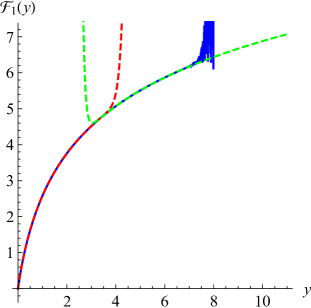
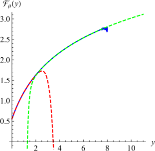
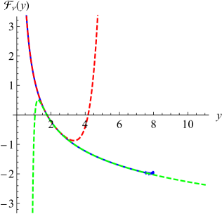
Figure 2: Left: The function $\mathcal{F}_{1}(y)$ (blue, solid), with its asymptotic expansions (red and green dashed). Middle: ibid. for $\mathcal{F}_{\mu}(y)$. Right: ibid. for $\mathcal{F}_{\nu}(y)$. Numerical measurements are presented on Figs. 5, 6 and 8.

Eq. (97) is equivalent to Eqs. (55) in WieseMajumdarRosso2010 , and (56) in DelormeWiese2016 .

The second function is for the drift proportional to $\mu$,

$${\mathcal{F}}_{\mu}(y):=\frac{{\mathbb{G}}_{\mu}(m,t)}{m\mathbb{G}_{0}(m,t)}+\partial_{\varepsilon}\bigg{|}_{\varepsilon=0}\left({\frac{m^{4\varepsilon}}{2D_{\varepsilon}y^{2\varepsilon}}}\right)\ .$$ (102)

It is evaluated as

$${\mathcal{F}}_{\mu}(y) = \frac{\left(y^{2}+1\right)[\mathcal{I}(y)-2]}{2y^{2}(1-y^{2})}+\frac{\sqrt{2\pi}\mathrm{e}^{\frac{y^{2}}{2}}\text{erfc}\left(\frac{y}{\sqrt{2}}\right)}{y\left(y^{2}-1\right)}$$ (103)

$$+\frac{1}{2}\Big{[}\ln(2)-\gamma_{\rm E}\Big{]}\ .$$

Its asymptotic expansions are

$${\mathcal{F}}_{\mu}(y) = \frac{1}{2}\Big{[}1-\gamma_{{\rm E}}+\ln(2)\Big{]}+\frac{1}{3}\sqrt{2\pi}y-\frac{y^{2}}{4}+\frac{1}{15}\sqrt{\frac{\pi}{2}}y^{3}$$ (104)

$$-\frac{y^{4}}{36}+\frac{1}{140}\sqrt{\frac{\pi}{2}}y^{5}-\frac{y^{6}}{360}+\frac{\sqrt{\frac{\pi}{2}}y^{7}}{1512}-\frac{y^{8}}{4200}$$

$$+\frac{\sqrt{\frac{\pi}{2}}y^{9}}{19008}-\frac{y^{10}}{56700}+\mathcal{O}(y^{11})\ ,$$

$${\mathcal{F}}_{\mu}(y) = \ln(2y)+\frac{\ln(2y^{2})+\gamma_{{\rm E}}-1}{2y^{2}}+\frac{3}{4y^{4}}-\frac{5}{4y^{6}}+\frac{35}{8y^{8}}$$ (105)

$$-\frac{189}{8y^{10}}+\mathcal{O}(y^{{-11}})\ .$$

Note that we added some strangely looking factors into the result (II.12). The factor $m\times m^{-\frac{2\varepsilon}{H}}=m^{\frac{1}{H}-1}$ accounts for the dimension of the diffusion constant, $m/D_{\varepsilon}\sim m\tau^{-2\varepsilon}$, and takes out the term $\ln(m)$ from $\mathcal{F}_{\mu}(y)$. We moved out also a remaining term $\sim\ln y$.

The third function is for the drift proportional to $\nu$,

$$\mathcal{F}_{\nu}(y):=\frac{\mathbb{\mathbb{G}}_{\nu}(y)}{{\mathbb{G}}_{0}(y)m}-\ln(y)\ .$$ (106)

It is evaluated as

$$\mathcal{F}_{\nu}(y)=\frac{\mathcal{I}(y)-2}{2y^{2}{}}+\frac{\ln(2)+\gamma_{\rm E}}{2}\ .$$ (107)

Its asymptotic expansions read

$$\mathcal{F}_{\nu}(y) = \frac{\sqrt{2\pi}}{y}+\frac{-3+\gamma_{\rm E}+\ln(2)}{2}-\frac{1}{3}\sqrt{\frac{\pi}{2}}y+\frac{y^{2}}{12}$$ (108)

$$-\frac{1}{60}\sqrt{\frac{\pi}{2}}y^{3}+\frac{y^{4}}{180}-\frac{1}{840}\sqrt{\frac{\pi}{2}}y^{5}+\frac{y^{6}}{2520}$$

$$-\frac{\sqrt{\frac{\pi}{2}}y^{7}}{12096}+\frac{y^{8}}{37800}-\frac{\sqrt{\frac{\pi}{2}}y^{9}}{190080}+\frac{y^{10}}{623700}$$

$$+\mathcal{O}(y^{11})$$

$$\mathcal{F}_{\nu}(y) = -\ln(y)+\frac{2\ln(y)+\gamma_{\rm E}+1+\ln(2)}{2y^{2}}+\frac{1}{4y^{4}}-\frac{1}{4y^{6}}$$ (109)

$$+\frac{5}{8y^{8}}-\frac{21}{8y^{10}}+\mathcal{O}(y^{-11})$$

Using Eq. (II.12) for small $y$, there is a problem when $\varepsilon\nu<0$, since then the combination (second-to-last term in the exponential)

$$-\varepsilon\nu my^{2\varepsilon}\left[\frac{1}{2}{+}\varepsilon\mathcal{F}_{\nu}(y)\right]\stackrel{{\scriptstyle y\to 0}}{{\longrightarrow}}-\varepsilon\nu m\sqrt{2\pi}y^{2\varepsilon-1}\approx-2\nu\sqrt{\pi}t^{H}.$$ (110)

diverges (at least for $\frac{1}{4}<H<\frac{1}{2}$), which is amplified since it appears inside the exponential. We propose to use the following Padé variant, which seems to work well numerically,

$$\left[\frac{1}{2}{+}\varepsilon\mathcal{F}_{\nu}(y)\right]\stackrel{{\scriptstyle\varepsilon<0,\,\nu>0}}{{-\!\!\!-\!\!\!-\!\!\!-\!\!\!-\!\!\!-\!\!\!\longrightarrow}}\frac{1}{2-4\varepsilon\mathcal{F}_{\nu}(y)}\ .$$ (111)

While $\mathcal{F}_{\nu}(y)$ diverges for small $y$, this is at leading order nothing but a normalization factor depending on $\nu t^{H}$.

All three functions $\mathcal{F}_{1}(y)$, $\mathcal{F}_{\mu}(y)$ and $\mathcal{F}_{\nu}(y)$ are measured in section 5, see figures 5, 6, and 8.

II.13 Absorption probability

From Eq. (64), we obtain, $\mathbf{P}_{\rm abs}(m,\alpha,\beta)$

$${\mathbf{P}}_{\rm abs}(m,\alpha,\beta)=\int_{0}^{\infty}\!\mathrm{d}t\,\mathbb{G}(m,tD_{\varepsilon})$$

$$=\int\limits_{0}^{\infty}\mathrm{d}t\,\exp\!\left(\!{-}\frac{m}{2}\!\left[\frac{\mu}{D_{\varepsilon}}{+}\nu\right]\!{-}\frac{t}{4}\left[\mu t^{-\varepsilon}{+}\nu t^{\varepsilon}\right]^{2}\right){\mathbb{G}}_{0}(m,tD_{\varepsilon})$$

$$+{\varepsilon}\int\limits_{0}^{\infty}\mathrm{d}t\exp\!\left({-\frac{m}{2}\beta-\frac{t}{4}\beta^{2}}\right)\times$$

$$\qquad\times\Big{[}{\mathbb{G}}_{1}(m,t)-\alpha\,{\mathbb{G}}_{\alpha}(m,t)-\beta{\mathbb{G}}_{\beta}(m,t)\Big{]}+\mathcal{O}(\varepsilon^{2})$$

$$=\exp\!\left(-\frac{m}{2}\left[\frac{\mu}{D_{\varepsilon}}+\nu\right]\right)$$

$$\times\Bigg{\{}\int\limits_{0}^{\infty}\mathrm{d}t\,\exp\!\left(-\frac{t}{4}\left[\mu t^{-\varepsilon}+\nu t^{\varepsilon}\right]^{2}\right){\mathbb{G}}_{0}(m,tD_{\varepsilon})$$

$$\qquad+{\varepsilon}\Big{[}\tilde{\mathbb{G}}_{1}(m,s)-\alpha\,\tilde{\mathbb{G}}_{\alpha}(m,s)-\beta\tilde{\mathbb{G}}_{\beta}(m,s)\Big{]}\Big{|}_{\sqrt{s}=|\beta|/2}\Bigg{\}}$$

$$+\mathcal{O}(\varepsilon^{2})\ .$$ (112)

Here $\tilde{\mathbb{G}}_{1}(m,s)$ is given by Eq. (67), $\tilde{\mathbb{G}}_{\alpha}(m,s)$ by Eq. (74), and $\tilde{\mathbb{G}}_{\beta}(m,s)$ by Eq. (77). We still need the integral

$$\int_{0}^{\infty}\mathrm{d}t\,\exp\!\left(-\frac{t}{4}\left[\mu t^{-\varepsilon}+\nu t^{\varepsilon}\right]^{2}\right){\mathbb{G}}_{0}(m,tD_{\varepsilon})$$ (114)

$$\qquad=\mathrm{e}^{-|\beta|m/(2\sqrt{D}_{\varepsilon})}+\frac{\alpha\beta}{2}\varepsilon\,{\mathbb{G}}_{3}(m,\beta)\ ,$$

$${\mathbb{G}}_{3}(m,\beta)=\int_{0}^{\infty}\mathrm{d}t\,\mathrm{e}^{-\frac{\beta^{2}t}{4}}t\ln(t){\mathbb{G}}_{0}(m,t)\ .~{}~{}~{}~{}~{}~{}~{}$$

The last expression can be calculated as

$${\mathbb{G}}_{3}(m,\beta):=\int_{0}^{\infty}\mathrm{d}t\,\mathrm{e}^{-\frac{\beta^{2}t}{4}}t\ln(t){\mathbb{G}}_{0}(m,t)$$ (115)

$$= \partial_{\kappa}\Big{|}_{\kappa=0}\int_{0}^{\infty}\mathrm{d}t\,\mathrm{e}^{-\frac{\beta^{2}t}{4}}t^{1+\kappa}{\mathbb{G}}_{0}(m,t)$$

$$= \partial_{\kappa}\Big{|}_{\kappa=0}\frac{|\beta|^{-\kappa-\frac{1}{2}}m^{\kappa+\frac{3}{2}}K_{\kappa-\frac{1}{2}}\!\left(\frac{m|\beta|}{2}\right)}{\sqrt{\pi}}$$

$$= -\frac{m^{3/2}\partial_{\kappa}\Big{|}_{\kappa=0}{K}_{\kappa-\frac{1}{2}}\!\left(\frac{|\beta|m}{2}\right)}{\sqrt{\pi|\beta|}}+\frac{m\mathrm{e}^{-\frac{|\beta|m}{2}}\ln\left(\frac{m}{|\beta|}\right)}{|\beta|}$$

$$= -\frac{me^{\frac{m\left|\beta\right|}{2}}\text{Ei}(-m\left|\beta\right|)}{\left|\beta\right|}+\frac{me^{-\frac{m\left|\beta\right|}{2}}\ln\left(\frac{m}{\left|\beta\right|}\right)}{\left|\beta\right|}$$

$$= \frac{m}{|\beta|}[-2\ln(|\beta|)-\gamma_{\rm E}]+\frac{1}{2}m^{2}\big{[}-2\ln(m)-\gamma_{\rm E}+2)\big{]}$$

$$+\mathcal{O}(m^{3})\ ,$$

where ${K}_{n}(z)$ denotes the modified Bessel function of the second kind. With the above formulas, Eq. (II.13) is rewritten as

$$\mathbf{P}_{\rm abs}(m,\alpha,\beta)=\mathrm{e}^{-{m(\beta+|\beta|)}/2}\bigg{\{}1+\varepsilon\,\mathrm{e}^{|\beta|m/2}\times$$ (116)

$$\times\bigg{[}\frac{\alpha\beta}{2}{\mathbb{G}}_{3}(m,\beta)+\frac{\alpha{+}\beta{+}|\beta|}{2}m(1{+}\ln\tau)\mathrm{e}^{-|\beta|m/2}$$

$$~{}~{}~{}~{}~{}~{}+\tilde{\mathbb{G}}_{1}(m,s)-\alpha\tilde{\mathbb{G}}_{\alpha}(m,s)-\beta\tilde{\mathbb{G}}_{\beta}(m,s)\bigg{]}_{\sqrt{s}=\frac{|\beta|}{2}}$$

$$+\mathcal{O}(\varepsilon^{2})\bigg{\}}\ .$$

We note the exact relations, which can be verified numerically,

$$\tilde{\mathbb{G}}_{1}(m,s)+2\sqrt{s}\,\tilde{\mathbb{G}}_{\beta}(m,s)=0\ ,$$ (117)

$${\mathbb{G}}_{3}(m,\beta)|\beta|+2\tilde{\mathbb{G}}_{\alpha}(m,s)$$

$$\qquad\qquad~{}~{}~{}~{}~{}-m(1+\ln\tau)\rm e^{-\frac{m\left|\beta\right|}{2}}\Big{|}_{\sqrt{s}=\frac{|\beta|}{2}}=0\ .$$ (118)

Let us analyse $\mathbf{P}_{\rm abs}$ separately for $\beta<0$ and $\beta>0$, starting with the former. Using both cancelations in Eqs. (117) and (II.13), we find

$$\mathbf{P}_{\rm abs}(\alpha,\beta<0)=1+\mathcal{O}(\varepsilon^{2})\ .$$ (119)

Thus there is no change in normalisation for a drift towards the absorbing boundary. For $\beta>0$, we find again with the use of Eqs. (117) and (II.13)

$$\mathbf{P}_{\rm abs}(\alpha,\beta>0)=\mathrm{e}^{-m\beta}\times$$

$$\times \!\!\bigg{\{}1+\varepsilon\,\bigg{[}(\alpha{+}\beta)m(1+\ln\tau)$$

$$+2\mathrm{e}^{\beta m/2}\Big{(}\tilde{\mathbb{G}}_{1}(m,s)-\alpha\tilde{\mathbb{G}}_{\alpha}(m,s)\Big{)}_{\sqrt{s}=\frac{\beta}{2}}\bigg{]}+\mathcal{O}(\varepsilon^{2})\bigg{\}}.$$

For what follows, we note regularity of the combination $\text{Ei}(-x)-\ln(x)-\gamma_{{\rm E}}$. We can write Eq. (II.13) as

$$\mathbf{P}_{\rm abs}(m,\alpha,\beta)=\mathrm{e}^{-m\beta}\times$$

$$\times \!\!\bigg{\{}1+\varepsilon\,\bigg{[}(m(\beta-\alpha)+2)\left(e^{\beta m}\text{Ei}(-m\beta)-\ln(\beta m)-\gamma_{\rm E}\right)$$

$$~{}~{}~{}~{}~{}~{}~{}~{}~{}~{}~{}~{}~{}~{}~{}-\alpha m(2\ln(\beta)+\gamma_{\rm E})+\beta m(2\ln(m)+\gamma_{\rm E})\bigg{]}$$

$$~{}~{}~{}+\mathcal{O}(\varepsilon^{2})\bigg{\}}$$

$$=\mathrm{e}^{-m\beta}\times$$ (121)

$$\times \!\!\bigg{\{}1+\varepsilon\,m\bigg{[}2(\beta{-}\alpha)\ln(\beta)-\gamma_{\rm E}(\alpha{+}3\beta)-2\beta+4\beta\ln(m)\bigg{]}$$

$$~{}~{}~{}+\mathcal{O}(\varepsilon^{2})+\mathcal{O}(m^{2}\varepsilon)\bigg{\}}\ .$$

As the asymptotic expansion in the last line shows, a common resummation is possible; passing to variables $\mu$ and $\nu$, it reads

$$\mathbf{P}_{\rm abs}(m,\mu,\nu) = \exp\!\Big{(}\!-m^{\frac{1}{H}-1}\mu\,\big{[}1+2(1-\gamma_{\rm E})\varepsilon\big{]}$$ (122)

$$~{}~{}~{}~{}-m^{\frac{1}{H}-1}\nu(\mu{+}\nu)^{\frac{1}{H}-2}\,\big{[}1{+}2(1{-}2\gamma_{\rm E})\varepsilon\big{]}\Big{)}\!\!$$

$$+\mathcal{O}(\varepsilon^{2})+\mathcal{O}(m^{2}\varepsilon)\ .$$

This formula represents the leading behavior of $\mathbf{P}_{\rm abs}(m,\mu,\nu)$ for small $m$; thus terms of order $\mathcal{O}(m^{2}\varepsilon)$ could be neglected. Note that the (inverse) powers of $H$ were chosen s.t. the resulting object is scale invariant. Expanding in $\varepsilon$ leads back to Eq. (II.13). One finally arrives at

$$\mathbf{P}_{\rm abs}(m,\mu,\nu) = \exp\!\Bigg{(}\!-m^{\frac{1}{H}-1}\bigg{\{}\mu\,\Big{[}1+2(1-\gamma_{\rm E})\varepsilon\Big{]}+\nu(\mu+\nu)^{\frac{1}{H}-2}\,\Big{[}1+2(1-2\gamma_{\rm E})\varepsilon\Big{]}\bigg{\}}$$ (123)

$$~{}~{}~{}~{}~{}~{}~{}~{}\,+\varepsilon\bigg{\{}2(m\nu+1)\Big{[}e^{m(\mu+\nu)}\text{Ei}\big{(}-m(\mu+\nu)\big{)}-\ln\big{(}m(\mu+\nu)\big{)}-\gamma_{\rm E}\Big{]}$$

$$~{}~{}~{}~{}~{}~{}~{}~{}~{}~{}~{}~{}~{}~{}~{}~{}~{}-2m(\mu+\nu)\Big{[}\ln\big{(}m(\mu+\nu)\big{)}+\gamma_{\rm E}-1\Big{]}\bigg{\}}\Bigg{)}+\mathcal{O}(\varepsilon^{2})\ .$$

In order that this formula be invariant under $m\to\lambda m$, $\mu\to\lambda^{1-\frac{1}{H}}\mu$ and $\nu\to\lambda^{-1}\nu$, we can either replace $m\mu$ by $m\mu^{\frac{H}{1-H}}$, or $m^{\frac{1}{H}-1}\mu$. The first version is

$$\mathbf{P}_{\rm abs}^{(a)}(m,\mu,\nu) = \exp\!\Bigg{(}\!-m^{\frac{1}{H}-1}\bigg{\{}\mu\,\Big{[}1+2(1-\gamma_{\rm E})\varepsilon\Big{]}+\nu\Big{(}\mu^{\frac{H}{1-H}}+\nu\Big{)}^{\frac{1}{H}-2}\,\Big{[}1+2(1-2\gamma_{\rm E})\varepsilon\Big{]}\bigg{\}}$$ (124)

$$~{}~{}~{}~{}~{}~{}~{}~{}\,+\varepsilon\bigg{\{}2(m\nu+1)\Big{[}e^{m\big{(}\mu^{\frac{H}{1-H}}+\nu\big{)}}\text{Ei}\Big{(}-m\big{(}\mu^{\frac{H}{1-H}}+\nu\big{)}\Big{)}-\ln\!\Big{(}m\big{(}\mu^{\frac{H}{1-H}}+\nu\big{)}\Big{)}-\gamma_{\rm E}\Big{]}$$

$$~{}~{}~{}~{}~{}~{}~{}~{}~{}~{}~{}~{}~{}~{}~{}~{}~{}-2m\Big{(}\mu^{\frac{H}{1-H}}+\nu\Big{)}\Big{[}\ln\!\Big{(}m\big{(}\mu^{\frac{H}{1-H}}+\nu\big{)}\Big{)}+\gamma_{\rm E}-1\Big{]}\bigg{\}}\Bigg{)}+\mathcal{O}(\varepsilon^{2})\ .$$

The alternative second version is

$$\mathbf{P}_{\rm abs}^{(b)}(m,\mu,\nu) = \exp\!\Bigg{(}\!-m^{\frac{1}{H}-1}\bigg{\{}\mu\,\Big{[}1+2(1-\gamma_{\rm E})\varepsilon\Big{]}+\nu(\mu^{\frac{H}{1-H}}+\nu)^{\frac{1}{H}-2}\,\Big{[}1+2(1-2\gamma_{\rm E})\varepsilon\Big{]}\bigg{\}}$$ (125)

$$~{}~{}~{}~{}~{}~{}~{}~{}\,+\varepsilon\bigg{\{}2(m\nu+1)\Big{[}e^{m^{\frac{1}{H}-1}\mu+m\nu}\text{Ei}\big{(}-m^{\frac{1}{H}-1}\mu-m\nu\big{)}-\ln\big{(}m^{\frac{1}{H}-1}\mu+m\nu\big{)}-\gamma_{\rm E}\Big{]}$$

$$~{}~{}~{}~{}~{}~{}~{}~{}~{}~{}~{}~{}~{}~{}~{}~{}~{}-\Big{(}m^{\frac{1}{H}-1}\mu+m\nu\Big{)}\Big{[}\ln\big{(}m^{\frac{1}{H}-1}\mu+m\nu\big{)}+\gamma_{\rm E}-1\Big{]}\bigg{\}}\Bigg{)}+\mathcal{O}(\varepsilon^{2})\ .$$

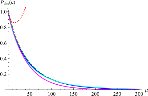
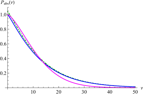
Figure 3: Example for the absorption probability as a function of $\mu$ at $\nu=0$ (left), and $\nu$ at $\mu=0$ (right). In all cases $m=0.1$. The blue solid line represents the result obtained by a direct numerical integration of Eq. (II.12), and adjusting the overall normalisation at $\mu=\nu=0$ to 1; this has the advantage that the combination $\mu m^{\frac{1}{H}-1}$ appears naturally. The green dashed curve is the same, without adjustment of normalisation. The red dotted curve (visible only on the left plot) is obtained using Eq. (123). The magenta curve is obtained using Eq. (124). The cyan curve is from Eq. (125), and is identical to the magenta one on the right plot.

From the appearance of fractal powers of $m$ and $\nu$ in Eq. (122), we suspect that both power series in $m\mu^{\frac{H}{1-H}}$ and $m^{\frac{1}{H}-1}\mu$ might appear. While numerical simulations could decide which version is a better approximation, only higher-order calculations would be able to settle the question.

II.14 Relation between the full propagator, first-passage times, and the distribution of the maximum

In this section, we demonstrate how the probability densities of three different observables follow from the same scaling function. This shows how our result can be used to find the probability distribution of both running maxima and first-passage times for fBM with linear and non-linear drift.

Let us start with the drift-free case, $\mu=\nu=0$.

1. In Ref. WieseMajumdarRosso2010 was calculated $\mathbb{P}_{+}(m,t)$, the normalised probability density to be at $m$, given $t$, when starting at $x_{0}$ close to 0 (in WieseMajumdarRosso2010 this quantity is denoted $P_{+}(x,t)$ with $m=x$). While $\mathbb{P}_{+}$ is a density in $m$, and thus should be denoted $P_{+}$ (cf. Tab. 1), it is the time derivative of a probability, see Eq. (131). This can be seen from its definition,

   $$\mathbb{P}_{+}(m,t):=\frac{P_{+}(m,t|x_{0})}{\int_{0}^{\infty}\mathrm{d}m\,P_{+}(m,t|x_{0})}\ ,$$ (126)

   and the asymptotic expansion at small $x_{0}$, (see e.g. WieseMajumdarRosso2010 , appendix C)

   $$\int_{0}^{\infty}\mathrm{d}m\,P_{+}(m,t|x_{0})\sim x_{0}^{\frac{1}{H}-1}\ ,$$ (127)

   which implies that $\mathbb{P}_{+}(m,t)$ has dimension $1/$time.

2. Here we consider the probability density to be absorbed at time $t$ when starting at $m$. This is a first-passage time, with distribution $\mathbb{P}_{\rm first}(m,t)$.

3. Third, let the process start at 0, and consider the distribution of the max $m$, given a total time $t$, $P_{\rm max}(m,t)$, denoted by $P^{T}_{H}(m)$ (with $t=T$) in Ref. DelormeWiese2016 .

All three objects have a scaling form depending on the same variable $y=\frac{m}{\sqrt{2}t^{H}}$:

$$\mathbb{P}_{\rm first}(m,t) = \frac{H}{t}\mathcal{P}_{\rm first}(y)\,\ ,$$ (128)

$$\mathbb{P}_{+}(m,t) = \frac{H}{t}\mathcal{P}_{+}(y)\ ,$$ (129)

$$P_{\rm max}(m,t) = \frac{1}{\sqrt{2}T^{H}}\mathcal{P}_{\rm max}(y)\ .$$ (130)

The factors of $H$ and $\sqrt{2}$ where chosen for later convenience. These objects are related. Denote $\mathbf{P}_{{\rm surv}}(m,t)$ the probability to start at $x=0$, and to survive in presence of an absorbing boundary at $m$ up to time $t$. Note that $\mathbf{P}_{{\rm surv}}(m,t)$ is a probability, whereas $\mathbb{P}_{{\rm first}}(m,t)$, $\mathbb{P}_{{+}}(m,t)$, and $P_{{\rm max}}(m,t)$ are densities, the first two in $t$, the latter in $m$. Then

$$\mathbb{P}_{+}(m,t) = \mathbb{P}_{\rm first}(m,t)=-\partial_{t}\mathbf{P}_{\rm surv}(m,t)\ ,~{}~{}~{}$$ (131)

$$P_{\rm max}(m,t) = \partial_{m}\mathbf{P}_{\rm surv}(m,t)\ .$$ (132)

Since $\mathbf{P}_{{\rm surv}}(m,t)$ is a probability, it is scale free, and scaling implies that

$$\mathbf{P}_{{\rm surv}}(m,t)=\mathbf{P}_{{\rm surv}}\!\left(y=\frac{m}{\sqrt{2}t^{H}}\right)\ .$$ (133)

Putting together Eqs. (131), (132) and (133) proves Eqs. (128) to (130), with

$$\mathcal{P}_{\rm first}(y) = \mathcal{P}_{+}(y)=y\mathbf{P}_{\rm surv}^{\prime}(y)$$ (134)

$$\mathcal{P}_{\rm max}(y) = \mathbf{P}_{\rm surv}^{\prime}(y)\ .$$ (135)

The scaling functions appearing are almost the same, differing by (innocent looking) factors of $t$ and $H$ and a (non-innocent looking) factor of $y$. However, when changing to the measure in $y$, all of them become identical. The survival probability in absence of a drift is given in Eqs. (63)-(64) of Ref. DelormeWiese2016 .

Let us finally add drift. Then the survival probability $\mathbf{P}_{\rm surv}(y,\tilde{u},v)$ depends on three variables introduced in Eqs. (12)-(15), setting there $x\to m$. Since $\tilde{u}=m\mu^{\frac{H}{1-H}}$, and $v=\nu m$ are both constants multiplying $m$, we can write $\mathbf{P}_{\rm surv}(y,\tilde{u},v)=\mathbf{P}_{\rm surv}(y,m)$. Using Eqs. (131) and (132), we find

$${\mathbb{P}}_{+}(m,t) = {\mathbb{P}}_{\rm first}(m,t)=-\frac{\mathrm{d}}{\mathrm{d}t}\mathbf{P}_{\rm surv}(y,m)$$ (136)

$$= \frac{H}{t}\partial_{y}\mathbf{P}_{\rm surv}(y,m)\ ,$$

$${P}_{\rm max}(m,t) = \frac{\mathrm{d}}{\mathrm{d}m}\mathbf{P}_{\rm surv}(y,m)$$ (137)

$$= \left[\frac{y}{m}\partial_{y}+\partial_{m}\right]\mathbf{P}_{\rm surv}(y,m)\ .$$

Passing to the measure in $y$, we obtain

$${\mathcal{P}}_{+}(y,m) = {\mathcal{P}}_{\rm first}(y,m)=y\partial_{y}\mathbf{P}_{\rm surv}(y,m)\ ,\qquad$$ (138)

$${\cal P}_{\rm max}(y,m) = \left[\partial_{y}+\frac{m}{y}\partial_{m}\right]\mathbf{P}_{\rm surv}(y,m)\ .$$ (139)

This set of equations allows us to express $\mathcal{P}_{\rm max}(y,m)$ as an integral over $\mathcal{P}_{+}(y,m)=\mathcal{P}_{\rm first}(y,m)$.

II.15 Tail of the distribution

Piterbarg PiterbargBook2015 states (section 11.3, page 85) that for a fBm defined on the interval $[0,1]$, with $\left<x_{1}^{2}\right>=1$, in the limit of $u\to\infty$,

$$\!\!\!\mathbf{P}(\mbox{max}_{0\leq t\leq 1}\,x_{t}>u)$$

$$\simeq\mathbf{\Psi}(u)\times\left\{\begin{array}[]{ccrcl}2&,&\quad H&=&1/2\\ 1&,&\quad H&>&1/2\\ \displaystyle\frac{{\cal H}_{2H}}{2H}2^{\frac{1}{2H}}u^{\frac{1}{H}-2}&,&~{}~{}H&<&1/2\\ \end{array}\right.\ .$$ (143)

$$\!\!\!\mathbf{\Psi}(u):=\frac{1}{\sqrt{2\pi}u}\exp\left(-\frac{u^{2}}{2}\right)\simeq\frac{1}{\sqrt{2\pi}}\int_{u}^{\infty}\exp\left(-\frac{x^{2}}{2}\right)\mathrm{d}x\ .$$

The estimate for $H<1/2$ seems to contain misprints: We find $\sigma(t):=\sqrt{\left<x_{t}^{2}\right>}=1-H|1-t|$ (i.e. $H$ instead of $2H$). Rescaling $t-1\to(t-1)\times 2^{\frac{1}{2H}}$ gives $\sigma(t)\to 1-H\times 2^{\frac{1}{2H}}\times|1-t|$, thus

$$\mbox{\bf P}(\mbox{max}_{0\leq t\leq 1}\,x_{t}>u)\simeq\frac{{\cal H}_{2H}}{2^{\frac{1}{2H}}H}u^{\frac{1}{H}-2}\mathbf{\Psi}(u)\ ,~{}~{}H<\frac{1}{2}.$$ (145)

Using the latter result, taking a derivative w.r.t. $u$, and passing to the measure in $y$, one obtains ${\cal P}(y)\equiv\mathcal{P}_{>}(y|m,\mu=\nu=0)\equiv{\cal P}_{\rm max}(y)$ (in terms of our variable $y$), in the limit of large $y$,

$${\cal P}(y)\simeq\frac{\mathrm{e}^{-\frac{y^{2}}{2}}}{\sqrt{2\pi}}\times\left\{\begin{array}[]{ccrcl}2&,&\quad H&=&1/2\\ 1&,&\quad H&>&1/2\\ \displaystyle\frac{{\cal H}_{2H}}{2^{\frac{1}{2H}}H}y^{\frac{1}{H}-2}&,&~{}~{}H&<&1/2\\ \end{array}\right.\ .\\$$ (146)

The Pickands constant ${{\cal H}_{2H}}$ has $\varepsilon$-expansion DelormeRossoWiese2017

$${{\cal H}_{2H}}=1-2\gamma_{{\rm E}}\varepsilon+{\cal O}(\varepsilon)^{2}\ .$$ (147)

How is this consistent with Eq. (II.12)? Taylor-expanding the latter for large $y$ yields

$${\cal P}(y)\simeq 2\frac{\mathrm{e}^{{-y^{2}/2}}}{\sqrt{2\pi}}\Big{\{}1 \!\!-\!\! \Big{[}1+\gamma_{{\rm E}}+2\ln(y)+\ln(2)\Big{]}{\varepsilon}$$ (148)

$$\!+\! {\cal O}(\varepsilon^{2})+{o}(y^{0})\Big{\}}\ .$$

In Ref. WieseMajumdarRosso2010 this was interpreted as ${\cal P}(y)\sim y^{-2\varepsilon}\mathrm{e}^{-y^{2}/2}$. Eq. (146) shows that this interpretation is incorrect. For large $y$, our expansion is almost the sum of the two contributions in Eq. (146) for $H\neq 1/2$,

$${\cal P}(y) \approx \frac{\mathrm{e}^{{-y^{2}/2}}}{\sqrt{2\pi}}\left[1+\frac{{\cal H}_{2H}}{2^{\frac{1}{2H}}H}y^{\frac{1}{H}-2}+...\right]$$ (149)

$$\simeq 2\frac{\mathrm{e}^{{-y^{2}/2}}}{\sqrt{2\pi}}\Big{\{}1-\Big{[}1+\gamma_{{\rm E}}+2\ln(y)-\ln(2)\Big{]}{\varepsilon}$$

$$~{}~{}~{}~{}~{}~{}~{}~{}~{}~{}~{}~{}~{}~{}~{}~{}~{}~{}+{\cal O}(\varepsilon^{2})+\mathcal{O}(y^{0})\Big{\}}\ .$$

Note the difference in sign for the $\ln(2)$ term between Eqs. (148) and (149), showing that the guess (149) slightly underestimates the amplitude for $\varepsilon<0$.

III Numerics

Figure 4: Left: First-passage time density $\mathcal{P}_{\rm first}(m,t)=\mathcal{P}(y)$ plotted as a function of $y$ as given in Eq. (9). In order to increase the resolution of the plot, we use overlapping bins with binsize $5\times 10^{5}$, with $y$ increasing by $10^{5}$ points for each bin; $m=0.1$. For various values of $H$ and $\mu$, numerical simulations are compared to the theory. As can be seen on this plot, and on the ratio between simulations and theory to the right, the relative error is about $3\%$ at the extreme points. Note that neglecting $\mathcal{F}_{1}(y)$ would lead for $H=0.4/0.6$ to an error of $15\%$, and for $H=0.33/0.67$ to an error of $25\%$.

Figure 5: Numerical estimate of $\mathcal{F}_{1}$. The black curve is the theoretical estimate (97), followed by a number of estimates using Eq. (152). Solid lines are for $m=0.1$, dashed ones for $m=1$. The symmetrised estimates (153) are in olive/cyan. The latter has minimal deviations from the theory. The inset shows a numerical estimate for $\mathcal{F}_{2}(y)$, as given by Eqs. (154) and (155). All curves are consistent, and let appear even the next-to-leading corrections. (Remind that changing the normalization is equivalent to adding a constant to $\mathcal{F}_{1}(y)$ or $\mathcal{F}_{2}(y)$). The strong curve-down for small and large $y$ are due to numerical problems.

III.1 Simulation protocol

Fractional Brownian motion can be simulated with the classical Davis-Harte (DH) algorithm DaviesHarte1987 ; DiekerPhD , whose algorithmic complexity (execution time) scales with system size $N$ as $N\ln N$. Here we use the adaptive bisection algorithm introduced and explained in Refs. WalterWiese2019a ; WalterWiese2019b . For $H=1/3$ its measured algorithmic complexity grows as $(\ln N)^{3}$, making it about 5000 times faster, and 10000 times less memory consuming than DH for an effective grid size of $N=2^{32}$.

To measure the functions $\mathcal{F}_{1}$, $\mathcal{F}_{\mu}$ and $\mathcal{F}_{\nu}$, which all depend on $y$ only, we

1. generate a (drift free) fBm $x_{t}$ with $x_{0}=0$, of length $N$; the latter corresponds to a time $T=1$.

2. add the drift terms to yield $z_{t}=x_{t}+\mu t+\nu t^{2H}$

3. for given $m$, find the first time $t$, s.t. $z_{t}=m$

4. evaluate $y=\frac{m}{\sqrt{2}t^{H}}$; add a point to the histogram of $y$.

This histogram misses values of $t>T=1$, i.e. $y<\frac{m}{\sqrt{2}}$.

We checked the procedure for Brownian motion (with $\nu\to 0$), where

$$\mathcal{P}(y|m,\mu)=\sqrt{\frac{2}{\pi}}\,\mathrm{e}^{-\frac{(\mu m+2y^{2})^{2}}{8y^{2}}}\ .$$ (150)

Note that this is a function of $y$ and $m\mu$ only, so that we can write

$$\mathcal{P}(y|m\mu)=\sqrt{\frac{2}{\pi}}\mathrm{e}^{-\frac{y^{2}}{2}}\times\mathrm{e}^{-\frac{m\mu}{2}}\mathrm{e}^{-\frac{(m\mu)^{2}}{8y^{2}}}\ .$$ (151)

For fBm, we measure $\mathcal{P}(y|m,\mu,\nu)$, and then extract $\mathcal{F}_{1}$, $\mathcal{F}_{\mu}$ and $\mathcal{F}_{\nu}$. Firstly,

$$\mathcal{F}_{1}^{\varepsilon}(y|m):=\frac{1}{\varepsilon}\ln\bigg{(}\mathcal{P}(y|m)y^{2-\frac{1}{H}}\mathrm{e}^{\frac{y^{2}}{2}}\bigg{)}\bigg{|}_{\mu=\nu=0}$$ (152)

and $\mathcal{F}_{1}^{\varepsilon}(y|m)=\mathcal{F}_{1}(y)+\mathcal{O}(\varepsilon^{2})$. The following combination is more precise, since terms even in $\varepsilon$ cancel,

$$\mathcal{F}_{1}^{\varepsilon,\rm sym}(y|m)=\frac{1}{2}\Big{[}\mathcal{F}_{1}^{\varepsilon}(y|m)+\mathcal{F}_{1}^{-\varepsilon}(y|m)\Big{]}+\mathcal{O}(\varepsilon^{2})\ .$$ (153)

The second-order correction can be estimated as

$$\mathcal{F}_{2}^{\varepsilon}(y|m):=\frac{1}{\varepsilon}\left[\mathcal{F}_{1}^{\varepsilon}(y|m)-\mathcal{F}_{1}(y|m)\right]+\mathcal{O}(\varepsilon)\ .$$ (154)

Its symmetrised version again suppresses subleading corrections,

$$\mathcal{F}_{2}^{\varepsilon,\rm sym}(y|m):=\frac{1}{2\varepsilon}\Big{[}\mathcal{F}_{1}^{\varepsilon}(y|m)-\mathcal{F}_{1}^{-\varepsilon}(y|m)\Big{]}+\mathcal{O}(\varepsilon^{2})\ .$$ (155)

The third order correction can be extracted as

$$\mathcal{F}_{3}^{\varepsilon}(y|m) := \frac{1}{2\varepsilon^{2}}\left[\mathcal{F}_{1}^{\varepsilon}(y|m)+\mathcal{F}_{1}^{-\varepsilon}(y|m)-2\mathcal{F}_{1}(y|m)\right]$$ (156)

$$+\mathcal{O}(\varepsilon)\ .$$

For the remaining functions $\mathcal{F}_{\mu}$ and $\mathcal{F}_{\nu}$, we can employ similar formulas; we have to decide how to subtract $\mathcal{F}_{1}$, numerically from the simulation, or analytically, i.e. by supplying numerically or analytically the denominator in

$$\mathcal{F}_{\mu}^{\varepsilon}(y|m,\mu) := -\frac{1}{\varepsilon}\bigg{[}\ln\bigg{(}\frac{\mathcal{P}(y|m,\mu,\nu=0)}{\mathcal{P}(y|m,\mu=\nu=0)}\bigg{)}\times\frac{y^{{-2\varepsilon}}}{\mu m^{{\frac{1}{H}-1}}}$$ (157)

$$\qquad+\frac{1}{2}+\frac{\mu}{4}\left(\frac{m}{2}\right)^{\!\!\frac{1}{H}-1}y^{{3-\frac{5}{2H}}}\bigg{]}\ ,$$

$$\mathcal{F}_{\nu}^{\varepsilon}(y|m) := -\frac{1}{\varepsilon}\bigg{[}\ln\bigg{(}\frac{\mathcal{P}(y|m,\mu=0,\nu)}{\mathcal{P}(y|m,\mu=\nu=0)}\bigg{)}\times\frac{y^{-2\varepsilon}}{\nu m}$$ (158)

$$\qquad+\frac{1}{2}+\frac{\nu m}{8}y^{-\varepsilon-2}\bigg{]}\ .$$

We can also work symmetrically

$$\mathcal{F}_{\mu}^{\varepsilon}(y|m):=-\frac{1}{\varepsilon}\!\left[\ln\!\bigg{(}\frac{\mathcal{P}(y|m,\mu,\nu{=}0)}{\mathcal{P}(y|m,-\mu,\nu{=}0)}\bigg{)}\frac{y^{{-2\varepsilon}}}{2\mu m^{{\frac{1}{H}-1}}}{+}\frac{1}{2}\right].$$ (159)

$$\mathcal{F}_{\nu}^{\varepsilon}(y|m):=-\frac{1}{\varepsilon}\left[\ln\bigg{(}\frac{\mathcal{P}(y|m,\mu{=}0,\nu)}{\mathcal{P}(y|m,\mu{=}0,-\nu)}\bigg{)}\frac{y^{-2\varepsilon}}{2\nu m}+\frac{1}{2}\right]\ .$$ (160)

Figure 6: Numerical estimate of $\mathcal{F}_{\mu}$. The black curve is the theoretical result (103). The colored curves are obtained using Eq. (159) with $\mu=\pm 1$ for $H=0.6$ and $H=0.67$, and $\mu=\pm 3$ for $H=0.33$ and $H=0.4$. Solid lines are for $m=0.1$, dashed ones for $m=1$. The symmetrised estimates (153) are in olive/cyan. The cyan curve using the equivalent of Eq. (153) with $H=0.4/0.6$ is our best numerical estimate of $\mathcal{F}_{\mu}(y).$ The inset shows the estimated second-order correction, analogous to Eqs. (154)-(155).

Finally, a more precise estimate of the theoretical curves is given by symmetrizing results for the same $|\varepsilon|$, using the analogue of Eq. (153).

Figure 7: Left: first-passage-time density plotted with overlapping bins as in Fig. 4 for various values of $H$ and non-linear drift $\nu$ compared to the theory given in Eq. (II.12). Right: Ratio of simulation and theoretical values.

Figure 8: Left: Numerical estimate of $\mathcal{F}_{\nu}$, using Eq. (160). The black curve is the theoretical prediction (107). The colored curves are simulation results using Eq. (160). Solid lines are for $m=0.1$, dashed ones for $m=1$. The cyan and olive curves are the symmetrised results using the equivalent of Eq. (153) for $H=0.4/0.6$ (cyan) and $H=0.33/0.67$ (olive). The former one is the best numerical estimate of the theory, and very close to the latter. The inset shows the estimated second-order corrections, analogous to Eqs. (154)-(155). There seem to be non-negligible corrections of order three. An almost perfect data collapse can be obtained for $m=0.1$ as $\varepsilon\mathcal{F}^{{\varepsilon}}_{{\nu}}(y)\simeq\mathcal{F}_{\nu}(y)\varepsilon+(2y^{-2}-4y^{-1}-6+y)\varepsilon^{2}+(3y-20)\varepsilon^{3}$, and for $m=1$ as $\varepsilon\mathcal{F}^{{\varepsilon}}_{{\nu}}(y)\simeq\mathcal{F}_{\nu}(y)\varepsilon+(y-1.7)(1.5\varepsilon^{2}-6\varepsilon^{3})$, see right figure. Since extrapolation problems mentioned around Eq. (111) become important for small $y$, this estimate is intended as a fit only, to show that the scatter on the left plot is consistent with higher-order corrections.

Below, we measure the three scaling functions $\mathcal{F}_{1}$, $\mathcal{F}_{\mu}$ and $\mathcal{F}_{\nu}$ for $H=0.33$, using our recently introduced adaptive-bisection algorithm WalterWiese2019a ; WalterWiese2019b . The latter starts out with an initial coarse grid of size $2^{g}$, which is then recursively refined up to a final gridsize of $2^{g+G}$. It gains its efficiency by only sampling necessary points, i.e. those close to the target.

The optimal values of $g$ and $G$ depend on $H$. We run simulations with the following choices: $H=0.33$ ($g=8$, $G=18$), $H=0.4$ ($g=10$, $G=14$), $H=0.6$ ($g=8$, $G=8$), and $H=0.67$ ($g=8$, $G=6$). Thanks to the adaptive bisection algorithm, we can maintain a resolution in $x$ of $10^{-3}$, with about 25 million samples at $H=0.33$, $H=0.6$ and $H=0.67$, and twice as much for $H=0.4$. As we will see below, this allows us to precisely validate our analytical predictions.

III.2 Simulation results

We show simulation results on Figs. 4 to 8. First, on figure 4 (left), we present results for the first-passage probability $\mathcal{P}(y|m,\mu,\nu=0)$, using $m=0.1$. The numerical results (in color) are compared to the predictions from Eq. (II.12). One sees that theory and simulations are in good quantitative agreement. This comparison is made more precise by plotting the ratio between simulation and theory on the right of Fig. 4.

The function $\mathcal{F}_{1}(y)$ is extracted on Fig. 5. We show simulations for $m=0.1$ (colored solid lines), and $m=1$ (colored dashed lines). The theoretical result (97) agrees with numerical simulations for all $H$, at both values of $m$. Using the symmetrized form (153) with $H=0.4/0.6$ shows a particularly good agreement. It allows us to extract the subleading correction via Eqs. (154) and (155). This is shown in the inset of Fig. 5; again the symmetrized estimate is the most precise. Note that the second-order correction is rather sensitive to the choice of $m$; more effort would be needed to estimate it properly. Also note that adding a constant to $\mathcal{F}_{1}(y)$ is equivalent to an overall change in normalization, thus one should concentrate on the shape of the cuves.

Using the data presented on Fig. 4, Fig. 6 shows the order-$\varepsilon$ correction $\mathcal{F}_{\mu}$ extracted via Eq. (159). The symmetrized estimate is rather close to the analytical result. The inset estimates the subleading correction. Again, estimates for $m=0.1$ (dashed lines) and $m=1$ (solid lines) are consistent, and a proper measure of the second-order correction would demand a higher numerical precision.

The results for non-linear drift $\nu$ are presented on Fig. 7, starting with the probability distribution $\mathcal{P}(y|m)$ (left), followed by the ratio between simulation and theory on the right, using $m=0.1$. The agreement is again good. From these data is extracted the function $\mathcal{F}_{\nu}(y)$ defined in Eq. (107), see Fig. 8. Note that $\mathcal{F}_{\nu}(y)$ is much larger than $\mathcal{F}_{\mu}(y)$ (Fig. 6), and diverges for small $y$. The subleading corrections to $\mathcal{F}_{\nu}(y)$ are not negligible, seemingly $m$-dependent, and estimated as well, allowing us to collapse all measured estimates on the theoretical curve.

In summary, we have measured all scaling functions with good to excellent precision, ensuring that the analytical results are correct.

IV Conclusion

In this article, we gave analytical results for fractional Brownican motion, both with a linear and a non-linear drift. Thanks to a novel simulation algorithm, we were able to verify the analytical predictions with grid sizes up to $N=2^{28}$, leading to a precise validation of our results.

Our predictions to first order in $H-1/2$ are precise, and many samples of very large systems are needed to see statistically significant deviations. We therefore hope that our formulas will find application in the analysis of data, as e.g. the stock market.

Another interesting question is how a trajectory depends on its history, i.e. prior knowledge of the process. We obtained analytical results also in this case, and will come back with its numerical validation in future work.

Our study can be generalised in other directions, as e.g. making the variance a stochastic process, as in ComteRenault1998 or in the rough-volatility model of Ref. GatheralJaissonRosenbaum2018 , which both use fBm in their modelling.

Acknowledgements

It is a pleasure to thank J.P. Bouchaud and F. Gorokhovik for discussions, G. Pruessner for help with the implementation, and M.T. Jaekel and A. Thomas for support with the cluster. B.W. thanks LPTENS and LPENS for hospitality.

References

- (1) S.N. Majumdar, G. Schehr and G. Wergen, Record statistics and persistence for a random walk with a drift, J. Phys. A 45 (2012) 355002.
- (2) G. Wergen, M. Bogner and J. Krug, Record statistics for biased random walks, with an application to financial data, Phys. Rev. E 83 (2011) 051109, arXiv:1103.0893.
- (3) P. Le Doussal and K.J. Wiese, Driven particle in a random landscape: disorder correlator, avalanche distribution and extreme value statistics of records, Phys. Rev. E 79 (2009) 051105, arXiv:0808.3217.
- (4) A. Rej, P. Seager and J.-P. Bouchaud, You are in a drawdown. When should you start worrying?, Wilmott (2018) 56–59, arXiv:1707.01457.
- (5) N. Shome, C.A. Cornell, P. Bazzurro and J.E. Carballo, Earthquakes, records, and nonlinear responses, Earthquake Spectra 14 (1998) 469–500.
- (6) S. Redner, A Guide to First-Passage Problems, Cambridge University Press, 2001.
- (7) E. J. Gumbel, Statistics of Extremes, Dover, 1958.
- (8) W. Feller, Introduction to Probability Theory and Its Applications, John Wiley & Sons, 1950.
- (9) W. Feller, Introduction to Probability Theory and Its Applications, Volume 2, John Wiley & Sons, 1969.
- (10) A.N. Borodin and P. Salminen, Handbook of Brownian Motion – Facts and Formulae, Birkhäuser, 2002.
- (11) J. Bertoin, Lévy Processes, Cambridge University Press, 1998.
- (12) K.J. Wiese, Span observables - “When is a foraging rabbit no longer hungry?”, J. Stat. Phys. 178 (2019) 625–643, arXiv:1903.06036.
- (13) I. Nourdin, Selected Aspects of Fractional Brownian Motion, Bocconi & Springer Series, 2012.
- (14) T. Sottinen, Fractional Brownian motion, random walks and binary market models, Finance and Stochastics 5 (2001) 343–355.
- (15) Y.G. Sinai, Distribution of the maximum of a fractional Brownian motion, Russian Math. Surveys 52 (1997) 359–378.
- (16) B.B. Mandelbrot and J.W. Van Ness, Fractional Brownian motions, fractional noises and applications, SIAM Review 10 (1968) 422–437.
- (17) J. Krug, Persistence of non-Markovian processes related to fractional Brownian motion, Markov Processes Relat. Fields 4 (1998) 509–516.
- (18) A.B. Dieker, Simulation of fractional Brownian motion, PhD thesis, University of Twente, 2004.
- (19) A.B. Dieker and M. Mandjes, On spectral simulation of fractional brownian motion, Probability in the Engineering and Informational Sciences 17 (2003) 417–434.
- (20) F. Aurzada, On the one-sided exit problem for fractional Brownian motion, Electron. Commun. Probab. 16 (2011) no. 36, 392–404.
- (21) L. Decreusefond and A.S. Üstünel, Fractional Brownian Motion: Theory And Applications. ESAIM: Proc. 5 (1998) 75-86
- (22) P.L. Krapivsky, K. Mallick and T. Sadhu, Dynamical properties of single-file diffusion, J. Stat. Mech. (2015) P09007, arXiv:1505.01287.
- (23) T. Sadhu and B. Derrida, Large deviation function of a tracer position in single file diffusion, J. Stat. Mech. 2015 (2015) P09008.
- (24) T. Sadhu and B. Derrida, Correlations of the density and of the current in non-equilibrium diffusive systems, J. Stat. Mech. 2016 (2016) 113202.
- (25) A. Zoia, A. Rosso and S.N. Majumdar, Asymptotic behavior of self-affine processes in semi-infinite domains, Phys. Rev. Lett. 102 (2009) 120602.
- (26) J.L.A. Dubbeldam, V.G. Rostiashvili, A. Milchev and T.A. Vilgis, Fractional Brownian motion approach to polymer translocation: The governing equation of motion, Phys. Rev. E 83 (2011) 011802.
- (27) V. Palyulin, T. Ala-Nissila and R. Metzler, Polymer translocation: the first two decades and the recent diversification, Soft Matter 10 (2014) 9016–9037.
- (28) J.-P. Bouchaud and A. Georges, Anomalous diffusion in disordered media: statistical mechanisms, models and physical applications, Phys. Rep. 195 (1990) 127–293.
- (29) E.E. Peters, Chaos and order in the capital markets, Wiley finance editions, Wiley, New York, 2 edition, 1996.
- (30) N.J. Cutland, P.E. Kopp and W. Willinger, Stock price returns and the Joseph effect: A fractional version of the Black-Scholes model, in E. Bolthausen, M. Dozzi and F. Russo, editors, Seminar on Stochastic Analysis, Random Fields and Applications, Volume 36 of Progress in Probability, pages 327–351, Birkhäuser Basel, 1995.
- (31) F. Biagini, Y Hu, B. Oksendal and T. Zhang, Stochastic Calculus for Fractional Brownian Motion and Applications, Springer Verlag, London, 2008.
- (32) B.B. Mandelbrot and J.R. Wallis, Noah, Joseph, and operational hydrology, Water Resour. Res 4 (1968) 909–918.
- (33) S. Gupta, A. Rosso and C. Texier, Dynamics of a tagged monomer: Effects of elastic pinning and harmonic absorption, Phys. Rev. Lett. 111 (2013) 210601.
- (34) E. Monte-Moreno and M. Hernández-Pajares, Occurrence of solar flares viewed with gps: Statistics and fractal nature, J. Geophys. Res. A 119 (2014) 9216–9227.
- (35) I. Simonsen, Measuring anti-correlations in the nordic electricity spot market by wavelets, Physica A 322 (2003) 597–606.
- (36) I. Norros, On the use of fractional brownian motion in the theory of connectionless networks, IEEE J. Sel. A. Commun. 13 (2006) 953–962.
- (37) K. Burnecki, E. Kepten, J. Janczura, I. Bronshtein, Y. Garini and A. Weron, Universal algorithm for identification of fractional Brownian motion. A case of telomere subdiffusion, Biophys J. 103 (2012) 1839–1847.
- (38) D. Ernst, M. Hellmann, J. Kohler and M. Weiss, Fractional Brownian motion in crowded fluids, Soft Matter 8 (2012) 4886–4889.
- (39) J.-H. Jeon, A.V. Chechkin and R. Metzler, First passage behaviour of fractional Brownian motion in two-dimensional wedge domains, EPL 94 (2011) 20008.
- (40) J.-H. Jeon, A.V. Chechkin and R. Metzler, First passage behaviour of multi-dimensional fractional Brownian motion and application to reaction phenomena, in R. Metzler, G. Oshanin, S. Redner, editors, First-Passage Phenomena and Their Applications, 175–202 World Scientific, Singapore, 2013, arXiv:1306.1667.
- (41) N.J. Cutland, P.E. Kopp and W. Willinger, Stock price returns and the Joseph effect: A fractional version of the Black-Scholes model, in E. Bolthausen, M. Dozzi and F. Russo, editors, Seminar on Stochastic Analysis, Random Fields and Applications, Volume 36 of Progress in Probability, pages 327–351, Birkhäuser Basel, 1995.
- (42) T. Guérin, N. Levernier, O. Bénichou and R. Voituriez, Mean first-passage times of non-Markovian random walkers in confinement, Nature 534 (2016) 356–359.
- (43) M. Delorme and K.J. Wiese, Perturbative expansion for the maximum of fractional Brownian motion, Phys. Rev. E 94 (2016) 012134, arXiv:1603.00651.
- (44) M. Delorme, Stochastic processes and disordered systems, around Brownian motion, PhD thesis, PSL Research University, 2016.
- (45) M. Delorme and K.J. Wiese, Maximum of a fractional Brownian motion: Analytic results from perturbation theory, Phys. Rev. Lett. 115 (2015) 210601, arXiv:1507.06238.
- (46) K. Es-Sebaiy, I. Ouassou and Y. Ouknine, Estimation of the drift of fractional Brownian motion, Statistics & Probability Letters 79 (2009) 1647–1653.
- (47) F. Black and M. Scholes, The pricing of options and corporate liabilities, J. Political Econ. 81 (1973) 637–654.
- (48) J.-P. Bouchaud and M. Potters, Theory of Financial Risk and Derivative Pricing, Cambridge University Press, 2009.
- (49) M. Kardar, G. Parisi and Y.-C. Zhang, Dynamic scaling of growing interfaces, Phys. Rev. Lett. 56 (1986) 889–892.
- (50) K.J. Wiese, On the perturbation expansion of the KPZ-equation, J. Stat. Phys. 93 (1998) 143–154, arXiv:cond-mat/9802068.
- (51) H.K. Janssen, U.C. Tauber and E. Frey, Exact results for the kardar-parisi-zhang equation with spatially correlated noise, Eur. Phys. J. B 9 (1999) 491–511.
- (52) E. Hopf, The partial differential equation , Comm. Pure Appl. Math. 3 (1950) 201–230.
- (53) J.D. Cole, On a quasi-linear parabolic equation occuring in aerodynamics, Q. Appl. Math. 9 (1951) 225–236.
- (54) K. Dȩbicki and P. Kisowski, A note on upper estimates for Pickands constants, Statist. Probab. Lett. 78 (2008) 2046–2051.
- (55) M. Delorme, A. Rosso and K.J. Wiese, Pickands’ constant at first order in an expansion around Brownian motion, J. Phys. A 50 (2017) 16LT04, arXiv:1609.07909.
- (56) L. de Haan and J. Pickands, Stationary min-stable processes, Probability Theory and Related Fields 72 (1986) 477–492.
- (57) A.J. Harper, Pickands’ constant does not equal , for small , Bernoulli (2017) 582–602, arXiv:1404.5505.
- (58) Z. Michna, Remarks on Pickands theorem, Probability and Mathematical Statististics 37 (2017) 373–393, arXiv:0904.3832.
- (59) J. Pickands III, Asymptotic properties of the maximum in a stationary Gaussian process, Trans. Amer. Math. Soc. 145 (1969) 75.
- (60) J. Pickands, The two-dimensional Poisson process and extremal processes, Journal of Applied Probability 8 (1971) 745–756.
- (61) J. Pickands, Statistical inference using extreme order statistics, Ann. Statist. 3 (1975) 119–131.
- (62) K.J. Wiese, S.N. Majumdar and A. Rosso, Perturbation theory for fractional Brownian motion in presence of absorbing boundaries, Phys. Rev. E 83 (2011) 061141, arXiv:1011.4807.
- (63) M. Delorme and K.J. Wiese, Extreme-value statistics of fractional Brownian motion bridges, Phys. Rev. E 94 (2016) 052105, arXiv:1605.04132.
- (64) K.J. Wiese, First passage in an interval for fractional Brownian motion, Phys. Rev. E 99 (2018) 032106, arXiv:1807.08807.
- (65) T. Sadhu, M. Delorme and K.J. Wiese, Generalized arcsine laws for fractional Brownian motion, Phys. Rev. Lett. 120 (2018) 040603, arXiv:1706.01675.
- (66) L. Benigni, C. Cosco, A. Shapira and K.J. Wiese, Hausdorff dimension of the record set of a fractional Brownian motion, Electron. Commun. Probab. 23 (2018) 1–8, arXiv:1706.09726.
- (67) V.I. Piterbarg, Twenty Lectures About Gaussian Processes, Atlantic Financial Press, London, New York, 2015.
- (68) R.B. Davies and D.S. Harte, Tests for hurst effect, Biometrika 74 (1987) 95–101.
- (69) B. Walter and K.J. Wiese, Monte Carlo sampler of first-passage times for fractional Brownian motion using adaptive bisections: Source code, hal-02270046 (2019).
- (70) B. Walter and K.J. Wiese, Sampling first passage times of fractional Brownian motion using adaptive bisections, (2019), arXiv:1908.11634.
- (71) F. Comte and E. Renault, Long memory in continuous-time stochastic volatility models, Mathematical Finance 8 (1998) 291–323.
- (72) J. Gatheral, T. Jaisson and M. Rosenbaum, Volatility is rough, Quant. Finance 18 (2018) 933–949.