Cell Model Approaches for Predicting the Swelling and Mechanical Properties of Polyelectrolyte Gels

Abstract

We present two successive mean-field approximations for describing the mechanical properties and the swelling equilibrium of polyelectrolyte gels in contact with a salt solution. The first mean-field approximation reduces the many-chain problem of a gel to a corresponding single chain problem. The second mean-field step integrates out the degrees of freedom of the flexible chain and the ions. It replaces the particle-based description of the polyelectrolyte with suitable charge distributions and an effective elasticity term. These simplifications result in a computationally very efficient Poisson-Boltzmann cell-gel description. Despite their simplicity, the single chain cell-gel model shows excellent and the PB model very good agreement with explicit molecular dynamics simulations of the reference periodic monodisperse network model for varying chain length, polymer charge fraction, and external reservoir salt concentrations. Comparisons of our models to the Katchalsky model reveal that our approach is superior for strongly charged chains and can also predict the bulk moduli more accurately. We further discuss chain length polydispersity effects, investigate changes in the solvent permittivity, and demonstrate the robustness of our approach to parameter variations coming from several modeling assumptions.

1 Polyelectrolyte Gels

Polyelectrolyte gels consist of crosslinked charged polymers. These gels can swell tremendously when placed in an aqueous environment and their reversible uptake of water is exploited in numerous applications such as superabsorbers, desalination agents [1, 2], cosmetics, pharmaceuticals [3, 4, 5], osmotic engines [6], or in agriculture [7, 8].

Optimizing polyelectrolyte gels to their respective application requires gel models which can yield accurate quantitative predictions of the swelling equilibria and their mechanical properties, a task that goes beyond known analytical approaches [9, 10, 11, 12, 13, 14, 15, 16, 17, 18]. Using the predicted pressure-volume curves the desalination performance of the gels as a function of, e.g., charge fraction or chain length can be assessed. Likewise, osmotic engines (gels that can translate differences in chemical potential to mechanical work) are another area for applications that benefit from quantitative predictions in order to optimize the engine efficiency prior to gel synthesis.

Macroscopic polyelectrolyte gels with monodisperse chain lengths have been simulated using molecular dynamics (MD) simulations with periodic boundary conditions (PBCs) (cf. periodic gel model) [19, 20, 21, 22, 23, 24, 25, 26, 27, 28, 29, 30]. These coarse-grained simulations provide predictions about mechanical and swelling properties of macroscopic gels and revealed microscopic insights about validities of various analytical predictions. Similar coarse-graining approaches already proved to be useful for microgels[14, 31, 32] as well.

Nevertheless, some features of real gels like polydispersity are hard to include into such models. In order to represent polydispersity faithfully, one would have to simulate a huge volume element with many chains of different length and a sufficiently large number of realizations. Huge particle-based simulations with more than $\leavevmode\nobreak\ 10^{5}$ monomers have been performed for investigating polydispersity in uncharged networks by [33] and [34]

To our knowledge, the only simulation study that treats polydispersity in charged polymer gels is that of [35]. Due to the computational cost of simulations with explicit charges Edgecombe et al. were only able to simulate gels with $\leavevmode\nobreak\ 10^{2}$ monomers  [35]. With this setup the polyelectrolyte chains are highly correlated since the small unit cell is periodically repeated. We compare the results obtained by Edgecombe qualitatively to a simple extension of or our models.

In a previous letter[36] we introduced two new mean-field gel models to which we refer to as the “single chain cell-gel model” (CGM = cell-gel model), and the “Poisson-Boltzmann (PB) CGM” in the following. We demonstrated the general applicability of the CGMs, and give a simple extension of the PB CGM to treat also weak (pH-sensitive) polyelectrolyte gels.

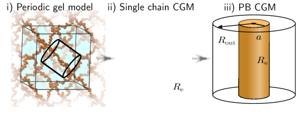
Figure 1: A schematic of the i) macroscopic gel; ii) single chain CGM; and iii) PB CGM of a macroscopic gel, which are in equilibrium with a salt reservoir. The symbols are introduced in the text.

For a quick recapitulation we illustrate in Figure 1 various levels of gel models: Starting from the periodic gel model i) we see in ii) the single chain CGM and iii) displays the second mean-field PB CGM [37]. In our models, the polymer chains are characterized by the number of monomers $N$ per chain, and the charge fraction per monomer $f\in[0,1]$. The reservoir, on the other hand, is characterized by the salt concentration $c_{\mathrm{salt}}^{\mathrm{res}}$, which is related to the reservoir concentrations of positive and negative ions $c_{\mathrm{salt}}^{\mathrm{res}}=c_{+}^{\mathrm{res}}=c_{-}^{\mathrm{res}}$ ensuring electroneutrality.

Two important features of all models i–iii) that deserve to be highlighted are the following two equilibrium conditions [12, 38]: First, the chemical potentials for all reservoir particle species $i$ are constant (in the following, we use species $i\in\{+,-\}$). Therefore, the chemical potentials (of each species $i$) in the gel ($\mu_{i}^{\mathrm{gel}}$) and in the reservoir ($\mu_{i}^{\mathrm{res}}$) are equal:

$$\mu_{i}^{\mathrm{gel}}=\mu_{i}^{\mathrm{res}}.$$ (1)

Second, the pressure of the gel ($P_{\mathrm{gel}}$) has to balance the pressure that is exerted on the system by the reservoir ($P_{\mathrm{res}}$):

$$P_{\mathrm{gel}}(V_{\mathrm{eq}})=P_{\mathrm{res}}.$$ (2)

In all models we approximate the reservoir pressure by the pressure of an ideal gas $P_{\mathrm{res}}\approx k_{\mathrm{B}}T\sum_{i}c^{\mathrm{res}}_{i}$ (unless specified otherwise). The gel, while in contact with a reservoir, is simulated at different volumes and the equilibrium volume $V_{\mathrm{eq}}$ is determined by eq. $\eqref{eq:pressure}$. In mechanical and chemical equilibrium the end-to-end distance is the equilibrium chain extension $R_{\mathrm{eq}}$.

The outline of the paper is as follows: First, we describe the periodic gel simulations which provide the benchmark data for our comparison. We then present in detail the single chain CGM and the PB CGM. We further compare the swelling equilibria and the elastic moduli of these models to the Katchalsky approach[29] and demonstrate the superiority of our new models. Additionally, we introduce polydispersity in our CGMs and investigate the effects that solvents of different polarity have on swelling.

2 Periodic Gel Model

Before describing the mean-field models, we briefly present the periodic gel simulations serving as a benchmark to evaluate the quality of our modeling approaches. The MD simulations are used to model periodically connected tetrafunctional strong gels on a coarse-grained level. In the periodic gel MD simulations we deal with crosslinked bead-spring polyelectrolytes in an implicit solvent. An example snapshot of a periodic gel can be seen in figure 1 i). All MD simulations presented in this paper have been performed using the MD simulation package ESPResSo [39] . We obtained the periodic gel benchmark data form simulations performed explicitly for this paper. The simulations are performed in full analogy to the setup described by Košovan[29]. In contrast to our previous publication[37] we did not use data from Košovan et al [29] since the grand canonical scheme was flawed. For clarity, we give a short recap on the simulation setup here: We simulate a unit cell of a tetrafunctional gel. The number of monomers per chain in our simulation varies: $N\in\{40,64,80\}$. The unit cell contains 16 chains and 8 nodes, i.e. in total $16N+8$ gel monomers. All particles interact via a Weeks-Chandler-Andersen (WCA) potential [40] with the effective particle size $\sigma=0.355\mathrm{nm}$ and strength of the interaction $\epsilon=1.0\,k_{\mathrm{B}}T$. Bonds connect the neighbouring monomers via FENE bonds [41], with the typical Kremer-Grest parameters [42] $k_{\mathrm{FENE}}=30.0\,k_{\mathrm{B}}T/\sigma^{2}$ and $R_{\mathrm{max}}=1.5\sigma$. Temperature is accounted for via a Langevin thermostat (at room temperature approx. $300\,\mathrm{K}$), while electrostatic interactions are calculated via the P3M method [43] tuned to an accuracy in the electrostatic force of at least $10^{-3}k_{\mathrm{B}}T/\sigma$ [44]. In our primitive model the relative electrostatic permittivity $\varepsilon_{\mathrm{r}}$ is chosen to be that of pure water at room temperature, i.e. $\varepsilon_{\mathrm{r}}\approx 80$. The Bjerrum length which corresponds to this choice is that of water at room temperature, i.e. $\lambda_{\mathrm{B}}=7.1\,\mathrm{}$ Å(unless otherwise noted). The simulation is performed in a semi-grand canonical ensemble[45] where salt and counterions are allowed to enter and leave the gel. The exchange of salt ions is performed by inserting pairs of salt ions. The acceptance probability for the insertion of one positive and one negative ion is[46]:

$$\text{acc}_{\text{insertion}}=\min\left(1,V^{2}c_{+}^{\mathrm{res}}c_{-}^{\mathrm{res}}\exp(\beta\mu^{\mathrm{res,ex}}_{s})\frac{1}{(N_{-}+1)(N_{+}+1)}\exp(-\beta\Delta E_{\mathrm{pot}})\right),$$ (3)

with $\beta=\frac{1}{k_{\mathrm{B}}T}$ and $\Delta E_{\mathrm{pot}}$ the potential energy change due to the Monte Carlo move. $N_{i}$ is the number of ions of species $i$ in the simulation volume $V$ and $c_{i}^{\mathrm{res}}$ is the concentration of species $i$ in the reservoir. The semi-grand canonical simulation makes use of the pair excess chemical potential in the reservoir $\mu^{\mathrm{res,ex}}_{s}=\mu^{\mathrm{res,ex}}_{+}+\mu^{\mathrm{res,ex}}_{-}$ for inserting a positive ($i=+$) and a negative ion ($i=-$) at the same time. The pair excess chemical potential is calculated in independent simulations of the reservoir (at different but fixed $c_{\mathrm{salt}}^{\mathrm{res}}$) via the Widom insertion method[46]. The adapted formula for determining the pair excess chemical potential for inserting a positive and a negative ion at the same time is:

$$\mu^{\mathrm{res,ex}}_{s}=-k_{\mathrm{B}}T\ln\left(\frac{1}{V^{2}}\int_{V}\int_{V}d^{3}r_{N+1}d^{3}r_{N+2}\langle\exp(-\beta\Delta E_{\mathrm{pot}})\rangle_{N}\right),$$ (4)

where $\langle\cdot\rangle_{N}$ is the canonical ensemble average over the N-particle configuration space[46] and where $\Delta E_{\mathrm{pot}}$ is the potential energy change due to the insertion of a positive and a negative ion. The simulated system is electroneutral at any time. As explained by [46] the two integrals in equation (4) are calculated via brute force sampling and inserting the ions at random positions inside the box.

This semi-grand canonical procedure ensures electrostatic neutrality as well as equality of the chemical potentials. For each simulation the volume and ensemble averaged virial pressure inside the gel is recorded yielding a pressure-volume ($PV$) curve (compare figure 2). The Coulomb part of the pressure is calculated as described by [47].

3 Single Chain Models

In contrast to the previously discussed expensive MD simulations of periodic gels, we proposed a reduction of the many-chain problem to a single chain problem in our recent publication [37]. In this section we describe common features of the (particle-based) single chain CGM and the PB CGM.

Using simple geometric considerations it is found that for a fully stretched tetrafunctional monodisperse gel the volume $V_{\mathrm{chain}}$, which is associated to a single chain, depends on the end-to-end distance $R_{\mathrm{e}}$ via the relation [29]

$$V_{\mathrm{chain}}=R_{\mathrm{e}}^{3}/A.$$ (5)

The denominator has the value $A=\sqrt{27}/4$ for a diamond lattice [29]. Whenever referring to the volume in the single chain models, we mean the volume $V_{\mathrm{chain}}$ per chain. For a not completely stretched gel, the denominator $A$ is non-trivially depending on the end-to-end distance[29]. For simplicity, we neglect this dependence and assume for the rest of the paper that $A$ is a constant (we discuss this point in the supporting information).

Relation $\eqref{eq:chain volume}$ connects the end-to-end distance and the volume which is available for a chain: on compression the end-to-end distance decreases since the ends of the polymer chains are brought closer together — at the same time also the volume which is available per chain shrinks.

Having fixed the volume which is accessible to a single chain in a periodic gel, we still need to decide on the geometry of the volume: In a macroscopic polyelectrolyte gel the monomers on one chain experience forces which originate from the electrostatic environment imposed by the other chains and from the elastic response to the crosslinking. Emulating this environment we choose a cylindrical volume and connect the chain ends through the cylinder top and bottom by applying PBCs.

Due to restrictions in the single chain CGM and application of PBCs (see section 3.2) the cylinder height needs to be $L(R_{\mathrm{e}})=R_{\mathrm{e}}+b$ with the bond length $b\approx 0.966\sigma\ll R_{\mathrm{e}}$. Here $b$ takes a value typical for the Kremer-Grest FENE potential[41]. In order to use results obtained for an affine compression of the cylinder (see section 3.1), and since $b$ is typically much smaller than $R_{\mathrm{e}}$, we approximate the volume available per chain via:

$$V_{\mathrm{chain}}\approx L(R_{\mathrm{e}})^{3}/A.$$ (6)

From the cylinder height and the cell volume (31) the outer cell radius $R_{\mathrm{out}}$ is given by:

$$R_{\mathrm{out}}=\sqrt{\frac{V_{\mathrm{chain}}(R_{\mathrm{e}})}{L(R_{\mathrm{e}})\pi}}=\sqrt{\frac{L(R_{\mathrm{e}})^{3}}{L(R_{\mathrm{e}})\pi A}}=\frac{L(R_{\mathrm{e}})}{\sqrt{\pi A}},$$ (7)

as depicted in figure 1. Since we consider only affine compressions we keep the aspect ratio $\alpha=R_{\mathrm{out}}/L$ constant in the single chain CGM and the PB CGM.

3.1 Pressures in an Affinely Compressed Cylinder

Applying the chain rule for the volume derivative of the free energy of the system $F_{\mathrm{gel}}$ (at fixed aspect ratio $\alpha$) we find the pressure in the cylindrical cell geometry as [48]:

$$P_{\mathrm{gel}} =-\frac{\partial F_{\mathrm{gel}}}{\partial V_{\mathrm{chain}}}\Bigg{|}_{\alpha}=-\frac{\partial F_{\mathrm{gel}}}{\partial R_{\mathrm{out}}}\frac{\partial R_{\mathrm{out}}}{\partial V_{\mathrm{chain}}}\Bigg{|}_{\alpha}-\frac{\partial F_{\mathrm{gel}}}{\partial L}\frac{\partial L}{\partial V_{\mathrm{chain}}}\Bigg{|}_{\alpha}$$ (8)

$$=\frac{2}{3}P_{\mathrm{side}}+\frac{1}{3}P_{\mathrm{cap}}.$$ (9)

This result allows to express the pressure of the cylindrical system via the pressure contribution $P_{\mathrm{cap}}$ from the top and a pressure contribution $P_{\mathrm{side}}$ from the side of the cylinder.

3.2 Particle-Based Single Chain CGM

Using the above described geometrical considerations, we introduce the first simplification for solving the many-chain problem of a periodic gel: the particle-based single chain CGM depicted in figure 1 ii). In the remainder of the text we call this model “single chain CGM”. Our single chain CGM consists of a single polyelectrolyte chain, confined to a cylinder of height $L(R_{\mathrm{e}})$ and radius $R_{\mathrm{out}}$. The first and last monomers of the single chain are bonded through the periodic boundary conditions and fixed to the cylinder center but are free to move along the cylinder axis. Applying PBCs mimics the electrostatic interactions in the gel where one end of the chain sees the beginning of the next chain, and where the fixed endpoints of the chain correspond to crosslinks in the gel. A single chain consists of $N$ monomers. The contour length of the chain is $R_{\mathrm{max}}=(N-1)b$, where $b$ is the average bond length. The particles in the particle-based single chain CGM interact with the same interactions and parameters as in the periodic gel model (FENE bonds, WCA potential, Langevin thermostat, P3M, semi-grand canonical ensemble). To compute the electrostatic forces and energies we use the P3M algorithm, with 3D periodic boundary conditions, tuned to an absolute accuracy [43] in the electrostatic force of at least $10^{-3}\frac{k_{\mathrm{B}}T}{\sigma}$. We compared the obtained forces of P3M with the more accurate MMM1D algorithm[49] designed for 1D periodic systems. We observed only small deviations compared to the P3M forces — this is especially true when using a gap in the x-y directions to separate the infinite cylinders.

In order to obtain a prediction for the swelling equilibrium we need to calculate the pressure inside the gel with the cap contribution $P_{\mathrm{cap}}$ and the side contribution $P_{\mathrm{side}}$ (see equation (9)). The caps of the cylinder are only imaginary and are not explicitly modeled. In the particle-based single chain CGM, the cap pressure is given by the ensemble average of the $(z,z)$ component of the instantaneous pressure tensor $P_{\mathrm{cap}}:=\langle\Pi_{(z,z)}\rangle$:

$$\Pi_{(z,z)}=\frac{\sum_{i}{m_{i}v_{i}^{(z)}v_{i}^{(z)}}}{V_{\mathrm{chain}}}+\frac{\sum_{j>i}{f_{ij}^{(z)}r_{ij}^{(z)}}}{V_{\mathrm{chain}}}+\Pi^{\text{Coulomb, P3M}}_{(z,z)}.$$

Here $V_{\mathrm{chain}}$ is the effective available volume, $m_{i}$ is the mass, $\vec{v}_{i}$ the velocity of particle $i$ (and the superscript $(z)$ denotes the z-component). $\vec{r}_{i,j}$ is the connection vector between particles $i$ and $j$. $\vec{f}_{i,j}$ is the pair force (excluding the electrostatic force) between particles $i$ and $j$. The last term is the zz-component of the instantaneous Coulomb pressure tensor[47] and accounts for the electrostatic interactions. Please note that the particle mass is irrelevant to the calculation of the ensemble averaged kinetic pressure tensor component $\langle\Pi_{\mathrm{kin},(z,z)}\rangle:=\langle\frac{\sum_{i}{m_{i}\vec{v}_{i}^{(z)}\vec{v}_{i}^{(z)}}}{V_{\mathrm{chain}}}\rangle$. The reason for this is that the velocities are Maxwell-Boltzmann distributed: The probability density to find a velocity vector $\vec{v}_{i}$ for particle $i$ is $p(\vec{v}_{i})=\left(\frac{m_{i}}{2\pi k_{\mathrm{B}}T}\right)^{3/2}\exp(-\beta\frac{m_{i}}{2}\vec{v}_{i}^{2})$. The probability density to find a certain component (e.g. the $z$ component) is $p({v}_{i}^{(z)})=\left(\frac{m_{i}}{2\pi k_{\mathrm{B}}T}\right)^{1/2}\exp(-\beta\frac{m_{i}}{2}{v_{i}^{(z)}}^{2})$. The ensemble average is, therefore, independent of the particle mass:

$$\langle\Pi_{\mathrm{kin},(z,z)}\rangle=\frac{1}{V_{\mathrm{chain}}}\sum_{i}{\int_{v_{i}^{(z)}=-\infty}^{\infty}m_{i}{v}_{i}^{(z)}{v}_{i}^{(z)}}p(v_{i}^{(z)})dv_{i}^{(z)}=\frac{\sum_{j}N_{\mathrm{j}}k_{\mathrm{B}}T}{V_{\mathrm{chain}}},$$ (10)

where the first sum runs over all particles $i$ and the last sum runs over all species $j$. This result is necessary in order to recover the limiting case of an ideal gas (which has no interactions) and for which the result of the isotropic pressure is well known: $P_{\mathrm{ideal}}=\langle\Pi_{\mathrm{kin},(z,z)}\rangle=\frac{\sum_{j}N_{j}k_{\mathrm{B}}T}{V}$. Therefore, we chose the arbitrary particle mass $m_{i}=1$ simulation unit.

The cylinder boundaries are the side walls. To constraint the particles in the cylinder all particles are repelled from the wall via a WCA interaction. The contribution of the pressure $P_{\mathrm{side}}$ acting on the side walls is directly measured as the average normal force on the outer wall per area. The side pressure mainly arises due to the pressure that the mobile ions exert onto the wall. Therefore, the side pressure could have also been obtained using the contact value theorem for the cylindrical cell model[50]. However, the contact theorem does not account for a possible interaction of the polymer chain with the wall and is therefore potentially less accurate.

In order to increase the accuracy of our description in the particle based models (namely the single chain CGM and the periodic gel model), we include the excess pressure in the pressure of the reservoir (for Bjerrum lengths $\lambda_{\mathrm{B}}>2\sigma$, i.e. $\varepsilon_{\mathrm{r}}<80$): $P_{\mathrm{res}}=k_{\mathrm{B}}T\sum_{i}c^{\mathrm{res}}_{i}+P^{\mathrm{ex,res}}$ (measured via independent MD simulations of the reservoir). In this case the excess pressure significantly lowers the pressure in the reservoir compared to the ideal gas pressure, due to the attractive nature of the electrostatic interaction.

Next, we present the second mean-field model which further simplifies the single chain CGM.

3.3 Poisson-Boltzmann CGM

The PB model uses a density based description of the polymer charges and the surrounding ions instead of a particle-based description. As before, the polymer and the ion densities are enclosed in a cylinder having an external radius $R_{\mathrm{out}}$ and a height of $R_{\mathrm{e}}+b$ as shown in figure 1 iii). The electrostatic environment in a gel is mimicked via periodically replicating the system along the z-axis. Therefore, we calculate the electrostatic interaction in the gel via solving the electrostatic problem for an infinite rod with prescribed charge density. In contrast to the original rod cell model[51, 52] our rod is penetrable to the ions. The maximal radial extension of the polymer density is denoted by the radius $a$ in figure 1 iii).

In the PB model the distribution of the monomers is, in principle, arbitrary with the following two restrictions: 1) the maximal extension $a$ needs to be smaller than the cell radius $R_{\mathrm{out}}$ and 2) the monomer distribution should be as realistic and as close as possible to that of a charged polymer bead-spring chain while maintaining the simplicity of the model. To fulfill restrictions 1) and 2) we use data from our previous single chain CGM simulations. From this data we extract a fitting curve for the average distance $\langle r\rangle_{\text{MD}}$ of the chain monomers from the cylinder axis as a function of $R_{\mathrm{e}}$:

$$\langle r\rangle_{\text{MD}}(R_{\mathrm{e}})=N\sigma\left(C_{1}\left(\frac{R_{\mathrm{e}}}{N\sigma}\right)^{2}+C_{2}\frac{R_{\mathrm{e}}}{N\sigma}+C_{3}\right),$$ (11)

with $C_{1}=-0.17$, $C_{2}=0.14$ and $C_{3}=0.03$ (fit to single chain CGM data for $N\in\{39,79,300\}$, $\varepsilon_{\mathrm{r}}=80$, for a fully charged chain without added salt).

This average distance of the monomers $\langle r\rangle_{\text{MD}}$ from the end-to-end vector is imposed on the monomer densities occurring in the PB model. To investigate the influence of the chosen monomer densities we investigate two distributions i) a rectangular distribution and in the supporting information a more realistic approximately Gaussian distribution with compact support ii). The probability density to find a monomer in a given distance $r$ from the cylinder axis has, in the case of a rectangular distribution, the form

$$p(\vec{r})=\mathcal{N}_{1}H(-(r-a)),$$ (12)

where $H(x)$ denotes the Heaviside function, and $\mathcal{N}_{1}$ a normalization such that $p(\vec{r})$ is a probability density. The normalization condition for $p(\vec{r})$ gives $\mathcal{N}_{1}=\frac{1}{\pi a^{2}L}$. The parameter $a$ is chosen such that the average distance from the end-to-end vector $\langle r\rangle=\int_{V_{\mathrm{chain}}}p(\vec{r})r\,\mathrm{d}V$ is equal to the average distance from the end-to-end vector which was observed in simulations of the single chain CGM: $\langle r\rangle\overset{!}{=}\langle r\rangle_{\text{MD}}$. Therefore, we obtain for the parameter $a=\frac{3}{2}\langle r\rangle_{\text{MD}}$.

The above probability density to find a monomer $p(\vec{r})$, together with the charge fraction $f$ and the number of monomers $N$ in the chain, imply a corresponding charge density $\rho_{f}(\vec{r})=-Nfe_{0}p(\vec{r})$, where $e_{0}$ is the absolute value of the elementary charge. This charge density is the key input to the Poisson-Boltzmann equation which describes the electrostatic interaction in the system:

$$\nabla^{2}\psi=-\frac{1}{\varepsilon_{\mathrm{r}}\epsilon_{0}}\left(q_{+}c_{+}(\vec{r})+q_{-}c_{-}(\vec{r})+\rho_{f}(\vec{r})\right),$$ (13)

where $\psi$ is the total electric potential, and $\varepsilon_{\mathrm{r}}$ is the relative permittivity. densities via $\rho_{i}(\vec{r})=c_{i}(\vec{r})q_{i}$) are given by standard Poisson-Boltzmann theory[53] (with the choice of the reservoir potential $\psi^{\mathrm{res}}=0$):

$$c_{i}(r)=c_{i}^{\mathrm{res}}e^{\frac{-q_{i}\psi(x,y,z)}{k_{\mathrm{B}}T}},$$ (14)

where $c_{i}^{\mathrm{res}}=c_{\mathrm{salt}}^{\mathrm{res}}$ are the ion densities in the reservoir of species $i$, where $i$ is either $+$ or $-$.

Since we model macroscopic gels we impose charge neutrality, hence, there is no flux of electric field through the surface of the cell. The two boundary conditions which we employ for solving the PB equation (13) are, therefore, that the radial electric field $E_{r}(r)$ is zero at $r=0$ and $r=R_{\mathrm{out}}$.

In the PB model the pressure has two contributions 1) the combined Maxwell and kinetic pressure and 2) the stretching pressure. For the standard PB theory the first contribution is given by[54]:

$$P_{\mathrm{side}}^{\text{ions}} =k_{\mathrm{B}}T\sum_{i}c_{i}(R)$$ (15)

$$P_{\mathrm{cap}}^{\text{ions}} =k_{\mathrm{B}}T\sum_{i}\langle c_{i}\rangle_{z}+\frac{\epsilon_{0}\varepsilon_{\mathrm{r}}}{2}\langle E_{r}^{2}\rangle_{z},$$ (16)

where $E_{r}=-\partial_{r}\psi(r)$ is the radial component of the electric field, $\epsilon_{0}$ is the vacuum permittivity, and where $\langle\mathcal{A}(r)\rangle_{z}=\frac{2\pi}{\pi R_{\mathrm{out}}^{2}}\int_{0}^{R_{\mathrm{out}}}r\mathcal{A}(r)\mathrm{d}r$ denotes the average taken over the cap. The side pressure is given by $k_{\mathrm{B}}T$ times the sum of the ion densities at the outer cylinder wall. This result is in agreement with the contact value theorem[50]. We want to note that the densities at the outer cylinder wall do not have to coincide with the densities in the reservoir. The second contribution is the stretching pressure which only acts on the cap. The stretching behavior of linear macromolecules under confinement is a delicate problem on its own and we refer the reader to further literature[55]. The simple stretching term which we use is motivated in the following. The stretching pressure is given as a volume derivative of a stretching free energy $F_{\mathrm{str}}$:

$$P_{\mathrm{cap}}^{\text{str}} =-\frac{\partial F_{\mathrm{str}}(R_{\mathrm{e}})}{\partial V_{\mathrm{chain}}}$$ (17)

$$=-\frac{\partial F_{\mathrm{str}}}{\partial L}\underbrace{\frac{\partial L}{\partial V_{\mathrm{chain}}}}_{1/(\pi R_{\mathrm{out}}^{2})}=-\frac{\partial F_{\mathrm{str}}}{\partial R_{\mathrm{e}}}\underbrace{\frac{\partial R_{\mathrm{e}}}{\partial L}}_{1}\frac{1}{\pi R_{\mathrm{out}}^{2}}.$$ (18)

Since the stretching free energy needs to contain a confinement contribution $F_{\mathrm{conf}}$ and a tensile chain contribution $F_{\mathrm{chain}}$ it consists of two terms: $F_{\mathrm{str}}=F_{\mathrm{chain}}+F_{\mathrm{conf}}$. Therefore one obtains:

$$P_{\mathrm{cap}}^{\text{str}}=-\frac{1}{\pi R_{\mathrm{out}}^{2}}\left(\frac{\partial F_{\mathrm{chain}}}{\partial R_{\mathrm{e}}}+\frac{\partial F_{\mathrm{conf}}}{\partial R_{\mathrm{e}}}\right).$$ (19)

The first term is given by the force extension curve of a freely jointed chain $-\frac{\partial F_{\mathrm{chain}}}{\partial R_{\mathrm{e}}}=\frac{k_{\mathrm{B}}T}{b}\mathcal{L}^{-1}\left(\frac{R_{\mathrm{e}}}{R_{\mathrm{max}}}\right)$ (with the inverse Langevin function $\mathcal{L}^{-1}$ or a numerical approximation[56] and the maximal contour length[57] $R_{\mathrm{max}}=(N-1)b$).

For the confinement free energy we use the result for a free ideal polymer: $F_{\text{conf}}=Bk_{\mathrm{B}}T\frac{Nb^{2}}{R_{\mathrm{e}}^{2}}$ [57, p. 115]. We choose the proportionality constant $B$ such that the stretching force is zero at the equilibrium extension: $\frac{\partial F_{\text{str}}}{\partial R_{\mathrm{e}}}\bigg{|}_{R_{0}}+\frac{\partial F_{\text{conf}}}{\partial R_{\mathrm{e}}}\bigg{|}_{R_{0}}=0$ yielding $B=\frac{R_{0}^{3}}{2Nb^{3}}\mathcal{L}^{-1}(\frac{R_{0}}{R_{\text{max}}})$. The final expression for the stretching pressure is:

$$P_{\mathrm{cap}}^{\text{str}}=\frac{1}{\pi R_{\mathrm{out}}^{2}}\frac{k_{\mathrm{B}}T}{b}\left(\frac{R_{0}^{3}}{R_{\mathrm{e}}^{3}}\mathcal{L}^{-1}\left(\frac{R_{0}}{R_{\mathrm{max}}}\right)-\mathcal{L}^{-1}\left(\frac{R_{\mathrm{e}}}{R_{\mathrm{max}}}\right)\right)$$ (20)

The equilibrium extension $R_{0}$ is a free parameter, and we use the relation $R_{0}=1.2bN^{0.588}$ which was found for a system of neutral chains interacting via a WCA potential [29].

In total the cap pressure is given by $P_{\mathrm{cap}}=P_{\mathrm{cap}}^{\mathrm{str}}+P_{\mathrm{cap}}^{\text{ions}}$, and together with eq. (9) one obtains the pressure in the gel model $P_{\mathrm{gel}}$. The PB model is expected to work well in aqueous solutions if there are no multivalent ions, high charge densities (e.g. at high compression of the gel) or high ionic concentrations present [58, 59]. Problems in PB theories arise due to neglecting ionic and excluded volume correlations. Also the simplistic stretching pressure $P_{\mathrm{cap}}^{\text{str}}$ (which is independent of the charge fraction and the salt concentration) adds a source of inaccuracy. These limitations are not present in our single chain CGM.

4 Results

4.1 Pressure-Volume Curves

All models which were described in the previous sections give pressure-volume curves (similar to stress-strain curves), see figure 2. In addition, we included $PV$ curves from the Katchalsky model which is a simple free energy model, for details please consult the papers authored by [29] and [10].

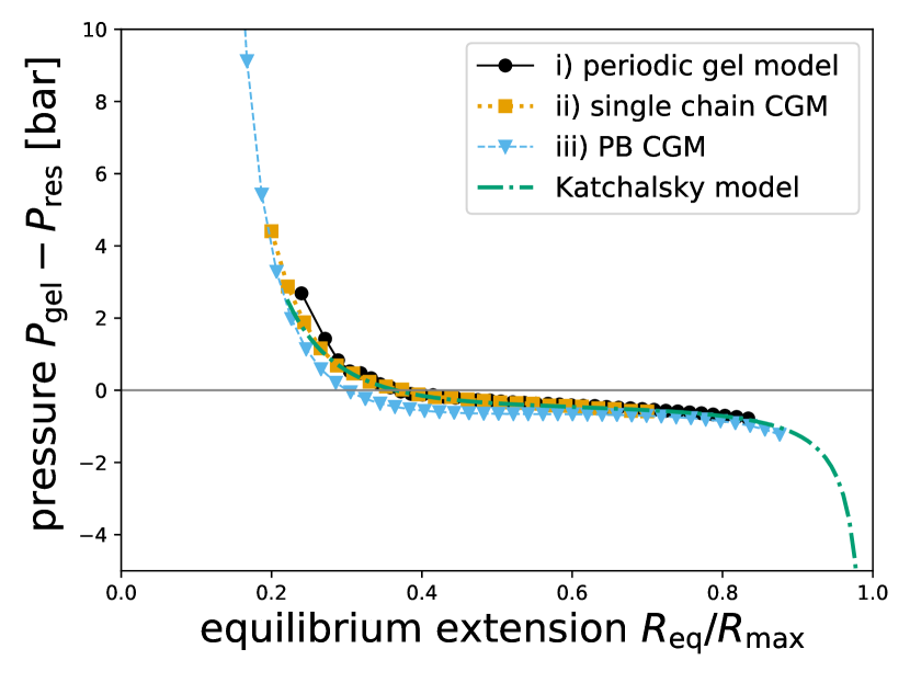
(a)

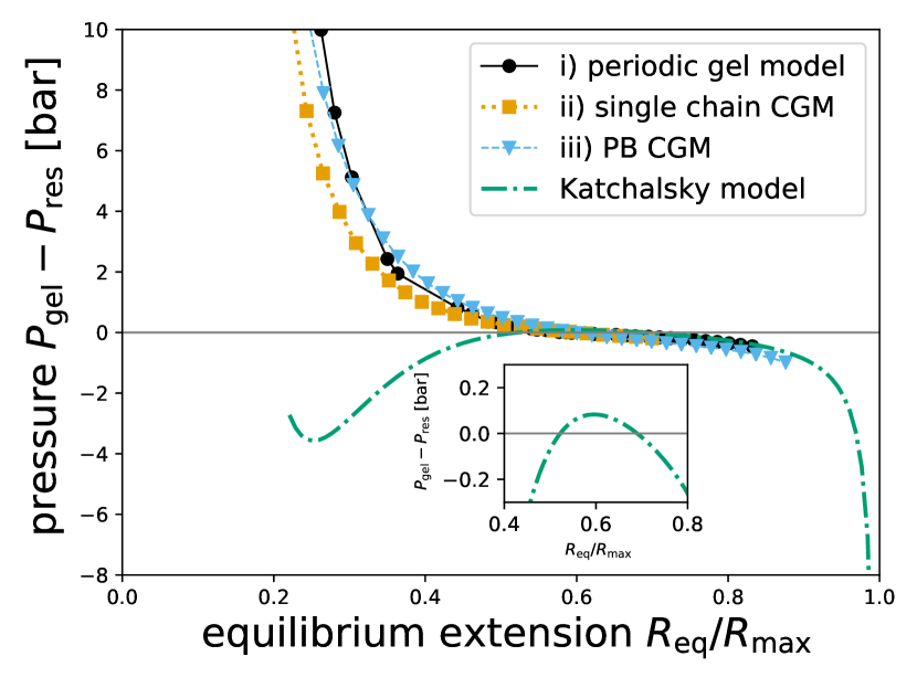
(b)

Figure 2: $P(R_{\mathrm{e}})$ curves for a) $f$=0.125 and b) $f$=1, both for $N$=64, $c_{\mathrm{salt}}^{\mathrm{res}}$=0.01 mol/l, $\lambda_{\mathrm{B}}=2\sigma$ (corresponds to $\varepsilon_{\mathrm{r}}=80$). The inset in figure b) shows the Katchalsky model data from figure b) enlarged. In the inset two zero crossings are visible. The abscissa is the equilibrium end-to-end distance divided by the maximum elongation of the chain and therefore parameterizes the volume per chain via eq. (31). As the end-to-end distance can be easily converted to a volume via equation (31) we refer to the $P(R_{\mathrm{e}})$ as $PV$ curve. $PV$ curves for other parameters can be found in the supplemental information.

Compared to the Katchalsky model, our new models work for all charge fractions. At high charge fractions ($f>0.5$  [29]) the Katchalsky model produces non-physical $PV$ curves which is obvious due to: a) the Katchalsky $PV$ curves have multiple zero crossings (see figure 2) and b) the Katchalsky $PV$ curves do not have a form compatible with the $PV$ curves of the periodic gel model. At high charge fractions the Katchalsky model fails due to the used electrostatic energy functional which is derived from a linearization of the PB equation[10]. Therefore, the this model is only of limited use for the prediction of desalination energy costs to gels with low charge fractions[2]. In contrast to the Katchalsky model, our new PB CGM gives monotonic $PV$ curves even for highly charged gels ($f>0.5$). All $PV$ curves used in this work can be found in the supplemental information. Additionally, our PB CGM also shows better agreement with the periodic gel model than the self-consistent field theory presented in Ref. [30, Figure 2]. Hence, the $PV$ curves could be used for an improved prediction of the energy costs for desalinating sea water using highly charged gels[2].

From figure 2 the swelling equilibrium for the corresponding gel can be obtained by identifying the zero crossing (where the reservoir pressure and the pressure in the gel balance). The dependence of the swelling equilibria on experimental conditions like the salt concentration or gel parameters like the charge fraction of the monomers are examined in the next section.

4.2 Swelling Equilibria

In figure 3 the scaled equilibrium extension $R_{\mathrm{eq}}/R_{\mathrm{max}}$ is shown as a function of the salt concentration in the reservoir ($c_{\mathrm{salt}}^{\mathrm{res}}$) and the charge fraction ($f$). In agreement with literature[19, 21, 15, 60, 23, 24, 26, 27, 61, 62, 28, 29] we find that the gel swells a) more with increased charge fraction $f$ and b) less with higher salt concentration in the reservoir.

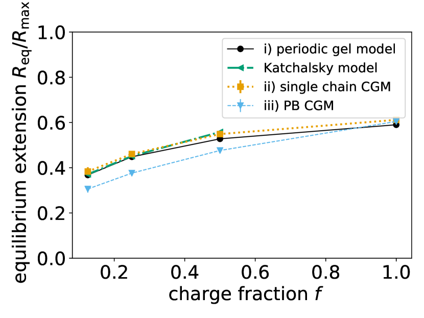
(a)

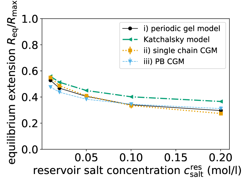
(b)

Figure 3: Comparison of swelling predictions of the periodic gel model i), the two new CGMs ii-iii) and the Katchalsky model for a polymer of chain length $N=64$ in aqueous solution ($\varepsilon_{\mathrm{r}}=80$). The equilibrium swelling $R_{\mathrm{eq}}$ as a) a function of the charge fraction $f$ for $c_{\mathrm{salt}}^{\mathrm{res}}=$0.01\text{\,}\mathrm{mol}\text{\,}{\mathrm{L}}^{-1}$$ and b) as a function of the reservoir salt concentration $c_{\mathrm{salt}}^{\mathrm{res}}$ for $f=0.5$. The equilibrium volume is determined by locating the volume where $P_{\mathrm{gel}}(V_{\mathrm{eq}})$ and $P_{\mathrm{res}}$ are equal by using a linear interpolation. The error bar is the width of the interval at which the intersection happens. The errorbar is typically smaller than symbol size. Note that in the first plot the points for the Katchalsky model do not cover the whole plot range. This is due to the fact that the Katchalsky model fails for these parameters [29].

In both subfigures of figure 3 we observe that the single chain CGM and the periodic gel model agree very well. Therefore, the usage of the single-chain CGM saves us an order of magnitude in CPU time without sacrificing the accuracy of the predictions of $R_{\mathrm{eq}}$. The PB CGM shows deviations from out reference data whose size depends on the chosen parameters, but in general the trend is reproduced. We find that the PB CGM also works for gels which are highly charged (where the Katchalsky model fails). In agreement with [29] we find, that the Katchalsky model offers very good gel swelling predictions for gels with low charge fraction. The exact quantification of how big the error of the different models is, however, a difficult problem. This arises from two facts:

• The PB model predictions can only be compared to a finite set of reference data which are computationally expensive to generate.

• The high dimensionality of the parameter space: predictions for gel swelling $R_{\mathrm{eq}}$ are made for different chain lengths, charge fractions, salt concentrations and dielectric permittivities. We observe that the PB and the Katchalsky model show differing suitability in predicting the swelling equilibrium in various parts of the parameter space.

For completeness, we include the swelling equilibria which were determined for all parameter combinations in the supplemental information. This data reveals that the PB CGM predicts too low swelling equilibria at low salt concentrations (compared to the periodic gel MD data) and too large swelling equilibria for highly charged gels $f\to 1$. In the following we want to explicitly name some simplifying assumptions made in the PB model which could cause these devations:

• The polymer charge density $\rho_{f}(\vec{r})$ in the PB model is, for simplicity, not dependent on the salt concentration or the charge fraction which are imposed in the model.

• The stretching contribution $P_{\mathrm{cap}}^{\text{str}}$ is independent of the salt concentration and the charge fraction $f$. For a charged polymer, we would expect a different stiffness depending on a) the salt concentration and b) the charge fraction. At low salt concentrations or high charge fractions the stiffness (or persistence length) should increase, resulting in a higher extension. Therefore, the force-extension of a polyelectrolyte should favor more stretched states at low salt concentrations or high charge fractions.

As mentioned above, the Katchalsky model does not provide valid predictions for high charge fractions which can be seen in the missing points in figure 3(a). Another tendency which can be see for some parameter combinations (e.g. in figure 3(b)) is that the Katchalsky model exhibits bigger deviations from the periodic gel model for higher salt concentrations. This could be related to the fact that the Debye-Hückel approximation works only well for low ion concentrations (below $0.01$ mol/l for 1:1 electrolytes[63] when used for predicting the ionic activity coefficient). Another possible reason could be that the elastic pressure contribution in the Katchalsky model is independent of charge fraction and salt concentration (similar to the PB model above).

Our new PB CGM also allows to obtain predictions for the equilibrium extension of long chains in a gel which were previously too expensive to simulate. For one set of parameters we show this prediction in figure 4 where the equilibrium end-to-end distance is plotted as a function of the chain length $N$. Additionally, we also show the predictions of the single chain CGM, the periodic gel model and the Katchalsky model. As one would expect the equilibrium end-to-end distance increases with chain length. The exact results, in figure 4, are important for the later treatment of polydisperse gels (as explained in section 4.6). At this point we want to note that the Katchalsky model fails for chain lengths $N\gtrsim 80$ (at $f=0.5$) and already shows significant deviations to the periodic gel model at $N=80$. As reported by Richter[64, Figure 70.] the electrostatic pressure contributions of the Katchalsky model are too negative for $f=0.5$ compared to the periodic gel model. These negative pressure contributions also introduce multiple zero-crossings in the $PV$ curve of the Katchalsky model for $N\gtrsim 80$ where the model fails.

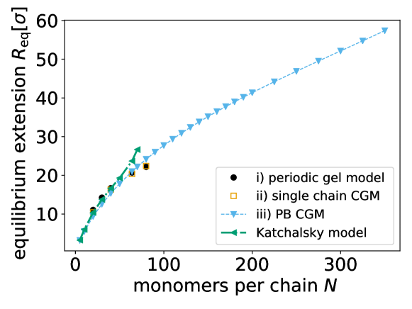
Figure 4: Predictions for the equilibrium end-to-end distance of monodisperse gels of different chain length $N$ for $f=0.5$, $\varepsilon_{\mathrm{r}}=80$ and $c_{\mathrm{salt}}^{\mathrm{res}}=0.1\,\mathrm{mol/l}$.

The overall agreement between the two new models and the expensive periodic gel simulations is evaluated in figure 5 which is a parametric plot with the periodic gel data on the abscissa and the data of the other models on the ordinate. A straight line with slope one would indicate perfect agreement with the periodic gel simulations (this “ideal line” is indicated with the label “linear” in figure 5). The single chain CGM fits the periodic gel data very good in the whole parameter space and therefore lies close to the “ideal line” (a fitted line $y(x)=mx$ through the single chain CGM data has the slope $m=1.01$ and a coefficient of determination $R^{2}=0.998$). The PB CGM in general has a similar trend as the periodic gel data but has deviations to the periodic gel data (a fitted line through the PB CGM data has slope $m=0.968$ and $R^{2}=0.98$). As outlined above, the data points where the swelling is below the “ideal line” are in tendency data at low salt concentration. PB CGM data which are above the “ideal line” are in tendency data at high charge fraction $f$. In contrast to the Katchalsky model our new models can be applied even at high charge fractions and high salt concentrations. The Katchalsky model data above the ideal line are due to deviations at high salt concentrations, while Katchalsky model data below the ideal line are due to deviations at high charge fraction. A fitted line to the Katchalsky model data including the outliers (excluding the outliers at $f=1$) has a slope $m=0.74$ ($m=1.07$) and a coefficient of determination $R^{2}=0.72$ ($R^{2}=0.992$).

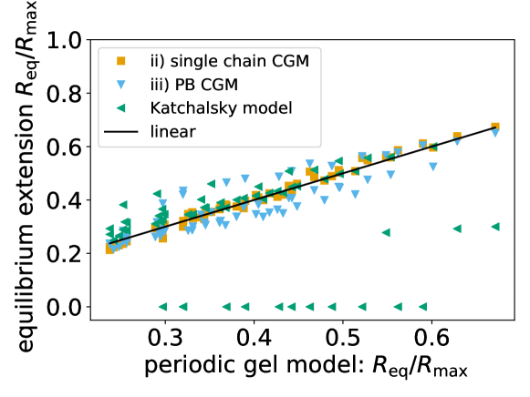
Figure 5: The swelling equilibria of the single chain CGM and the PB CGM compared to the more detailed periodic gel model. The results are presented for a wide set of parameter combinations with $\varepsilon_{\mathrm{r}}=80$, $N\in\{40,64,80\}$, $f\in\{0.125,0.25,0.5,1\}$ and $c_{\mathrm{salt}}^{\mathrm{res}}\in\{0.01,0.02,0.05,0.1,0.2\}$ $\mathrm{mol}\text{\,}{\mathrm{L}}^{-1}$. The linear function has the form $y(x)=x$ and is referred to as “ideal (prediction) line”. Note that the Katchalsky model produces outliers at high charge fractions which go hand in hand with high degrees of swelling in the periodic gel model. In order to show the failure of the Katchalsky model we included data points for which the Katchalsky model failed to give a prediction. For illustration purposes we assign those data points to $R_{\mathrm{eq}}/R_{\mathrm{max}}=0$. We want to note that our comparison includes more charge fractions below $f=0.5$ than above. This might lead to the wrong impression that the Katchalsky model works in most of the charge fraction although it does not work for $f>0.5$.

As we see in figure 5 there seems to be “scattering” around the predicted periodic gel data which serve as benchmark. The “scattering” of the different model data around the periodic gel data in figure 5 is due to the models not working perfectly and projecting the results obtained in a three-dimensional parameter space: $\{c_{\mathrm{salt}}^{\mathrm{res}},N,f\}$ onto a one dimensional abscissa. While there is no “scattering” (in the sense of a strongly non-monotonic behavior) of the data around the ideal line for a single parameter set (e.g. $R_{\mathrm{eq}}(\{c_{\mathrm{salt}}^{\mathrm{res}}\},N=\mathrm{fix},f=\mathrm{fix})/R_{\mathrm{max}}$) there is apparent “scattering” when plotting two data sets (e.g. $R_{\mathrm{eq}}(\{c_{\mathrm{salt}}^{\mathrm{res}}\},N=40,f=0.125)/R_{\mathrm{max}}$ and $R_{\mathrm{eq}}(\{c_{\mathrm{salt}}^{\mathrm{res}}\},N=80,f=1)/R_{\mathrm{max}}$, see supplemental infromation) from separate regions of the parameter space together in figure 5. This “scattering” does not mean that predictions of the models vary in a strongly non-monotonic when only varying one parameter.

Deviations between the simplified models and the periodic gel model are either due to simplified descriptions of the interactions (as discussed above) or at least in part due to the fact that the parameter $A$ is not a constant but rather a function of the end-to-end distance[29]. This non-affine behavior exists in the periodic gel model and probably in real polymer networks[65]. Therefore, a refined theory would also take into account that the compression of a gel is not affine and would deal with $A(R_{\mathrm{e}})$. In the supporting information we investigate the effect of changing $A$ on the predicted end-to-end distance in the PB CGM and find, however, that the influence is small.

4.3 Bulk Modulus

Mechanical properties are important, for example, when evaluating the energetic costs for desalination with polymer gels[2]. One mechanical property of interest is the isothermal bulk modulus $K$ of a gel as a measure for the mechanical strength:

$$K=-V\frac{\partial P_{\mathrm{gel}}}{\partial V}\approx-V\frac{\Delta P_{\mathrm{gel}}}{\Delta V}.$$ (21)

In the case of the single chain CGMs we use $V_{\mathrm{chain}}$ instead of $V$. The volume derivative of the pressure curve is approximately calculated via the finite difference quotient of the points which are at the intersection of the reservoir and system pressure.

The scaling behavior of the shear modulus is connected to the scaling of the bulk modulus $K$ via the Poisson ratio[66] $\nu$:

$$K=\frac{2(1+\nu)}{3(1-2\nu)}G.$$ (22)

The scaling analysis by Barrat et al.[38] (which is also based on the pressure balance of the osmotic and the elastic pressure using the ideal Donnan equilibrium) predicts that in swelling equilibrium the shear modulus of a polymer gel is given by $G=k_{\mathrm{B}}T\left(\frac{c_{m}}{N}\right)\left(\frac{R_{\mathrm{eq}}^{2}}{Nb^{2}}\right)$, where $c_{m}=N/R_{\mathrm{eq}}^{3}$ is the monomer concentration in the gel in equilibrium[38], $N$ the number of monomers per chain, and $b$ the size of the monomer. The equilibrium end-to-end distance scales with the number of monomers per chain $R_{\mathrm{eq}}\propto N^{\nu_{\text{gel}}}$, where $\nu_{\text{gel}}$ is a Flory exponent. Note that the Flory exponent of a free chain and the Flory exponent $\nu_{\text{gel}}$ do not agree in general (compare Barrat et al.[38]). Using this we obtain $G\propto N^{-(\nu_{\text{gel}}+1)}$. In salt free solution we further have the following relation for the equilibrium end-to-end distance in a gel[38] $R_{\mathrm{eq}}\propto Nb$. Therefore, we expect $K\propto G\propto 1/N^{2}$. For a gel in contact with a saline solution and in a good solvent we expect[38] $R_{\mathrm{eq}}\propto bN^{3/5}$ which therefore alters the scaling prediction $K\propto G\propto N^{-8/5}=N^{-1.6}$.

The bulk modulus obtained by the PB CGM is displayed in figure 6 together with values obtained from the single chain CGM, the periodic gel model, and the Katchalsky model. For the two particle-based models the $PV$-curve and the errors in the pressure are recorded during the simulation. The resulting error in the bulk modulus is then calculated according to error propagation in the volume $V$ and the slope $\partial P_{\mathrm{gel}}/\partial V$. The used formula is:

$$\Delta K=\left|\left(\frac{\partial P_{\mathrm{gel}}}{\partial V}\right)_{\mathrm{eq}}\right|\Delta V_{\mathrm{eq}}+V_{\mathrm{eq}}\Delta\left(\frac{\partial P_{\mathrm{gel}}}{\partial V}\right)_{\mathrm{eq}},$$ (23)

where the symbol $\Delta$ denotes that the error margin is positive. The error margins $\Delta V_{\mathrm{eq}}$ and $\Delta\left(\frac{\partial P_{\mathrm{gel}}}{\partial V}\right)_{\mathrm{eq}}$ are determined using the error bars of the pressure next to the equilibrium point.

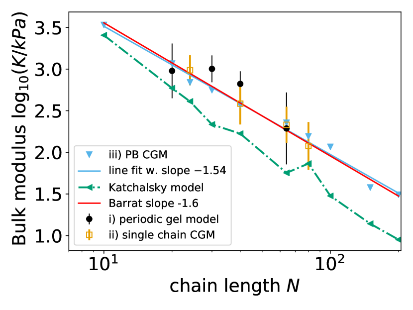
(a)

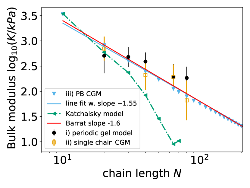
(b)

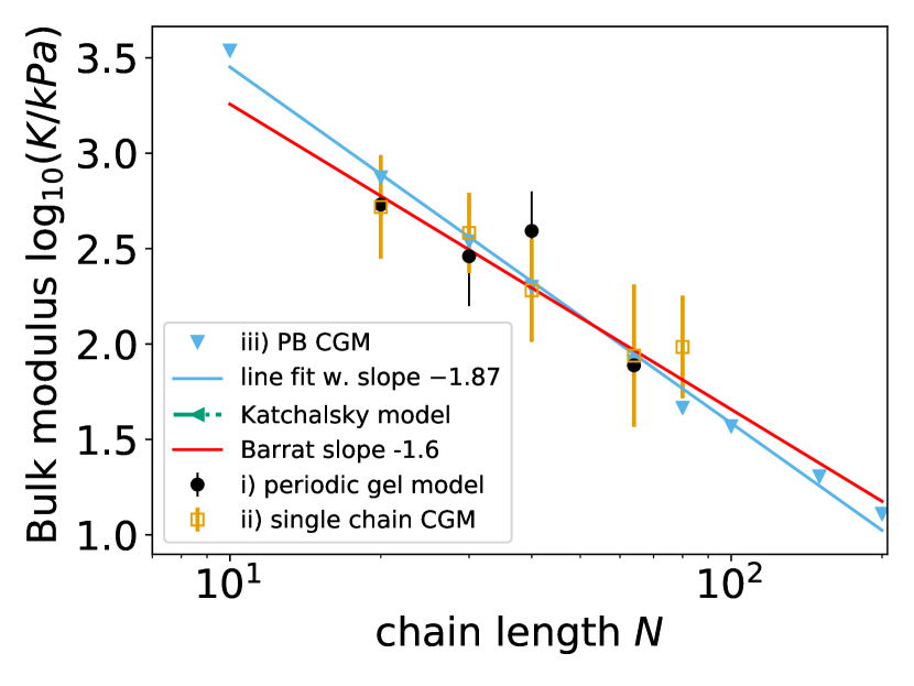
(c)

Figure 6: Predictions of periodic gel model i), the two single chain CGMs ii–iii) and the Katchalsky model for the bulk moduli $K$ of monodisperse gels of different chain length $N$ for a) $f=0.125$, b) $f=0.5$ and c) $f=1$ at $\varepsilon_{\mathrm{r}}=80$ and $c_{\mathrm{salt}}^{\mathrm{res}}=0.1\,\mathrm{mol/l}$. For $f=1$ the Katchalsky model fails and therefore there are no data points.

In our PB CGM we find scaling exponents $K\propto N^{-1.54\pm 0.06}$ (for $f=0.125$), $K\propto N^{-1.55\pm 0.03}$ (for $f$=0.5) or $K\propto N^{-1.87\pm 0.06}$ (for $f$=1) via fitting to data $N>5$. The PB CGM data for the bulk modulus do not follow a perfect power law as predicted by Barrat[38], there are deviations at very small chain lengths and large chain lengths. Therefore, the scaling exponents for the $N$ dependence of the bulk modulus should be taken with care. We observe that the scaling exponents of the bulk modulus with $N$ are close to the scaling prediction $K\propto G\propto N^{-1.6}$ when the gels carry a low charge fraction. We also find that the PB CGM, the single chain CGM, and the periodic gel model agree within error bars. The Katchalsky model, on the other hand, shows significant deviations to the periodic gel model, it deviates from the particle-based model predictions both at charge fraction $f$=0.125 and $f$=0.5 or even fails at $f=1$ (where we have no Katchalsky model prediction). For low charge fractions the slope of the Katchalsky data is still compatible with Barrat’s scaling prediction while for charge fraction $f=0.5$ the deviation to Barrats scaling prediction and the periodic gel data is already significant. We conclude that our new models provide an improved description of the mechanical properties of gels at intermediate or high charge fractions ($f\geq 0.5$) when compared to the Katchalsky model.

We also want to note that the error bars on the bulk modulus for the particle-based models (obtained via propagation of error) are big. Due to this fact, we do not fit scaling exponents to the particle-based model data. It seems that in figure 6 b) the periodic gel model would have a different best fit line than the PB CGM. One possible reason for this could be that the PB CGM uses a stretching pressure which is derived from an ideal model, neglecting a possible salt dependence or charge fraction dependence of this pressure contribution. A chain length dependent correction to the ideal behaviour would also change the bulk modulus predicted with equation (21).

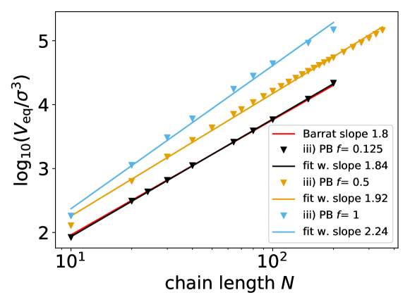
Figure 7: PB CGM predictions for the chain length ($N$) dependence of the volume per chain of monodisperse gels at $\varepsilon_{\mathrm{r}}=80$ and $c_{\mathrm{salt}}^{\mathrm{res}}=0.1\,\mathrm{mol/l}$. The different charge fractions $f$ are encoded via color as indicated in the legend. The volume is calculated according to eq. (31) using the equilibrium end-to-end distance. The scaling prediction by Barrat is shown in red (with fitted y-intercept to the PB model data for $f=0.125$). We expect the idealized model by Barrat[38] to work best for low charge fractions.

In figure 7 we also display the volume at swelling equilibrium as a function of $N$. Like Barrat, we assume that the volume of the gel is proportional to the end-to-end distance cubed[38]. We expect the following scaling behavior in swelling equilibrium $V_{\mathrm{eq}}\propto N^{3}$ (in the salt free case) and $V_{\mathrm{eq}}\propto N^{9/5}\approx N^{1.8}$ (in the case of added salt)[38]. As one can see in figure 7 the PB CGM predicts a scaling of $V_{\mathrm{eq}}\propto N^{2.24\pm 0.065}$ (for $f=1$), $V_{\mathrm{eq}}\propto N^{1.92\pm 0.03}$ (for $f=0.5$) and $V_{\mathrm{eq}}\propto N^{1.84\pm 0.01}$ (for $f=0.125$) which is close to Barrat‘s prediction for added the salt ($V_{\mathrm{eq}}\propto N^{9/5}=N^{1.8}$). In the case of high charge fraction $f=1$ we do not expect the model by Barrat to work anymore since ions are treated on the ideal level[38]. Therefore, the scaling exponent in the PB model is different to the prediction by Barrat[38]. Since $V_{\mathrm{eq}}\propto R_{\mathrm{eq}}^{3}\propto N^{3\nu_{\text{gel}}}$, we find “effective” Flory exponents $\nu_{\text{gel}}=0.613\pm 0.01$ (for $f=0.125$), $\nu_{\text{gel}}=0.64\pm 0.01$ (for $f=0.5$) or $\nu_{\text{gel}}=0.75\pm 0.03$ (for $f=1$). For highly charged gels the electrostatic interactions stretch the gel more and the swelling increases (resulting in a higher $\nu_{\text{gel}}$).

4.4 Influence of the Relative Permittivity

The relative permittivity $\varepsilon_{\mathrm{r}}$ controls the strength of the electrostatic interaction in the implicit solvent approach. Around $\varepsilon_{\mathrm{r}}\approx 80$ both, the single chain CGM and the PB CGM, agree well in their prediction for the swelling equilibrium (see figure 8). The results for the PB CGM and the single chain CGM are shown in figure 8.

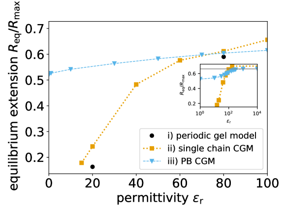
Figure 8: PB CGM and single chain CGM predictions for the equilibrium end-to-end distance of monodisperse gels for $N=64$, $f=1$ and $c_{\mathrm{salt}}^{\mathrm{res}}=0.01\,\mathrm{mol/l}$ at various different relative permittivities $\varepsilon_{\mathrm{r}}$. Additionally, we confirm the accuracy of the single chain CGM simulations by providing two periodic gel data points for the swelling equilibrium at $\varepsilon_{\mathrm{r}}=80$ and $\varepsilon_{\mathrm{r}}=20$. The inset shows the limiting behavior of the PB CGM and the single chain CGM for large relative permittivities. In this limit salt is partitioned according to the ideal Donnan behavior (grey line) for the PB CGM. The data point at $\varepsilon_{\mathrm{r}}=\infty$ for the single chain CGM is obtained by switching the electrostatic interactions off.

For lower values of $\varepsilon_{\mathrm{r}}$ the electrostatic interactions become so strong that ion correlation effects occur [67]. These correlation effects cannot be captured by the mean-field Poisson-Boltzmann approach [67] and produce a stronger collapse of the gel than predicted by the PB CGM.

The effect of varying $\varepsilon_{\mathrm{r}}$ was previously investigated (for periodic gel model) by Schneider et al. [68] who observed a similar trend. We also confirm the accuracy of the single chain CGM by comparing our data to those of periodic gel simulations at $\varepsilon_{\mathrm{r}}=80$ and $\varepsilon_{\mathrm{r}}=20$.

At larger relative permittivities, electrostatic interactions diminish. In the limit of $\varepsilon_{\mathrm{r}}\to\infty$ the electrostatic interaction energy approaches zero, and the salt is partitioned according to the ideal Donnan prediction[29]:

$$c_{\mathrm{salt}}^{\mathrm{gel}}=\sqrt{\left(\frac{fc_{m}}{2}\right)^{2}+{c_{\mathrm{salt}}^{\mathrm{res}}}^{2}}-\frac{fc_{m}}{2}.$$ (24)

Here $c_{\mathrm{salt}}^{\mathrm{gel}}$ is the salt concentration inside the gel, $c_{\mathrm{salt}}^{\mathrm{res}}$ the salt concentration in the reservoir and $c_{m}$ the concentration of monomers in the gel.

This salt partitioning allows to predict the behavior in the limit $\varepsilon_{\mathrm{r}}\to\infty$ since then ions can be treated as an ideal gas, and the pressure contributions $P_{\mathrm{cap}}$ and $P_{\mathrm{side}}$ can be evaluated easily via the homogeneous densities (the electric field goes to zero for $\varepsilon_{\mathrm{r}}\to\infty$). The Donnan partitioning is used for calculating the cell model pressures and yields the grey line in the inset in figure 8. In figure 8 it is visible that the PB CGM and the single chain CGM swell slightly different for $\varepsilon_{\mathrm{r}}\to\infty$. This difference of roughly 6 % in $R_{\mathrm{e}}/R_{\mathrm{max}}$ appears due to different stretching pressures in both models and possibly due to the neglect of excluded volume interactions in the PB model.

We want to point out that the strong collapse in solvents with low dielectric constant cannot be accurately represented by theories which treat the electrostatic interactions only on an approximate ideal level (ensuring electroneutrality via Donnan equilibrium) or on a Debye-Hückel level, as is done for example in the approaches by Katchalsky [10], Tanaka [11], Khokhlov [12], or the model by Barrat[38].

4.5 Mass-Based Degree of Swelling (for Monodisperse Gels)

For better comparison with experimental results it is instructive to introduce a mapping from the predicted end-to-end distances $R_{\mathrm{eq}}$ to the mass the gel has in swelling equilibrium. This facilitates the comparison of experimental results where the swelling equilibrium is often reported as a fraction of the mass of the solvent in the swollen state divided by the mass of the dry state of the gel $Q_{m}=m_{\text{solvent uptake}}/m_{\text{dry}}$. This mapping requires some modeling assumptions. First, the mass of the dry state is determined by the number of monomers $N$ per chain, the total number of chains $N_{\mathrm{chains}}$ in the gel and the mass of the monomers $m_{0}$:

$$m_{\text{dry}}=m(N)N_{\mathrm{chains}},$$ (25)

where $m(N)=Nm_{0}$ is the mass of one chain with N monomers. The monomer mass depends on the experimental preparation and we choose $m_{0}=$94 u so that the monomers represent sodium acrylate. The second modeling assumption is that we can measure the mass of the solvent in the swollen gel via its volume and an approximate density $\rho_{\mathrm{w}}\approx 1\,\mathrm{kg/l}$ which is close to that of pure water:

$$m_{\text{solvent uptake}}=V_{\mathrm{chain}}(N)\rho_{\mathrm{w}}N_{\mathrm{chains}},$$ (26)

where $V_{\mathrm{chain}}(N)$ is the volume per chain given by eq. (31). This volume per chain is predicted, e.g., by the single chain CGM or the PB CGM (compare figure  4). The volume of the gel is obtained by multiplying $V_{\mathrm{chain}}$ with the number of chains $N_{\mathrm{chains}}$ (which cancels in the calculation of $Q_{m}$).

This simple mapping allows for the prediction of mass-based degrees of swelling[6]. The results for monodisperse gels are shown in figure 10 as a black curve. In the following, we generalize our mapping of the (mass based) degree of swelling and introduce polydispersity effects.

4.6 Chain Length Polydispersity

So far we have only treated monodisperse macroscopic gels. In reality, however, most gels are highly polydisperse[69, 34, 33, 70]. Properties of polymeric systems typically depend on the chain length polydispersity and in many applications this feature may be used to improve material properties for a given application[71, p.10]. Nevertheless, polydispersity is often negelected in theoretical considerations and a monodisperse molar mass distribution is assumed.

Chain length heterogeneity is a parameter for which data for comparison cannot be easily obtained via MD/MC simulations of periodic charged gels: A simulation of a heterogeneous gel would require prohibitively time-consuming simulations with a huge simulation box to realize a representative distribution of the chain length distribution. Additionally, a strict comparison to experiments is difficult because the exact chain length distribution in typical experiments is unknown due to the insufficient characterization of the topology of real gels. We employ here a simple approach where we assume that a polydisperse macroscopic gel can be described by partitioning the total volume into sub-cells which contain chains of possibly different length in each cell. Given that we know the probability mass function (pmf) for the polymer length in a gel $p(N)$ (see e.g. Panyukov and Rabin[69]) we can then easily obtain the degree of swelling for a polydisperse gel. In the studies by [33] and [34] the strand length distribution is exponential or close to exponential and therefore very broad. As outlined by [70] random crosslinking gives a Flory-Schulz distributed chain length polydispersity, i.e. a geometrical distribution or in good approximation an exponential distribution[70]. For simplicity, we assume that the chain length is distributed according to this geometric or Flory-Schulz distribution[72, 73]:

$$p_{a}(N)=a(1-a)^{N-1},$$ (27)

where $0<a<1$ is a fit parameter for a given gel and $N\in\mathbb{N}$ is the number of monomers per chain. An illustration of the corresponding probability mass function can be found in figure 9.

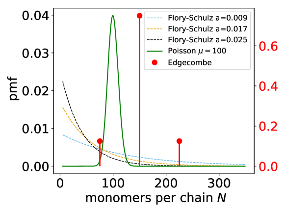
Figure 9: The figure shows the different probability mass functions which we use in this paper: the geometrical distribution (Flory-Schulz), the Poisson distribution and the distribution in accordance with Edgecombe[35]. The Flory-Schulz distribution is shown for different parameters $a$. The pmfs are only defined for integer values $N$, the lines serves only as a guide to the eye. The three shown values of the parameter $a$ are the minimal used $a$, the maximally used $a$ and the median of the used values of $a$. The values of $a$ which we chose, all guarantee that at least 90 % of the chains have a chain length between $N=5$ and $N=350$ for which we have data $R_{\mathrm{eq}}(N)$ (see figure 4). This means we choose values of $a$ such that $\sum_{N=5}^{350}p_{a}(N)>0.9$. Note that the distribution from Edgecome is only nonzero for three values of $N$ and therefore the probability for those values is bigger than usual compared to the other distributions. Therefore, the pmf of Edgecombe has its own ordinate axis in red.

For demonstration purposes we also investigate a Poisson distribution $p_{\mu}(N)=\exp(-\mu)\frac{\mu^{N}}{N!}$, where $\mu>0$ is the average value $E(N)=\mu$ and the variance $\mathrm{Var}(N)=\mu$. This narrow distribution of chain lengths is for example obtained via chain polymerizations[71]. Finally, we also investigate the distribution that was used by [35]:

$$p_{N_{\mathrm{short}},N_{\mathrm{medium}},N_{\mathrm{long}}}(N)=\begin{cases}1/8\text{ if N=}N_{\mathrm{short}}\\ 3/4\text{ if N=}N_{\mathrm{medium}}\\ 1/8\text{ if N=}N_{\mathrm{long}}\\ 0\text{ else.}\\ \end{cases}$$ (28)

For the different chain lengths which occur in this probability mass function, we have the restriction $\frac{1}{2}(N_{\mathrm{short}}+N_{\mathrm{long}})=N_{\mathrm{medium}}$ [35]. We always choose $N_{\mathrm{short}}=0.5N_{\mathrm{medium}}$ and $N_{\mathrm{long}}=1.5N_{\mathrm{medium}}$ like Edgecombe et al.

Using the geometrical pmf, the Poisson pmf or the Edgecombe pmf we weight the contributions of cells with different polymer chain lengths in order to predict the (mass-based) degree of swelling of the gel: The degree of swelling for a polydisperse gel is given via the following ratio

$$\langle Q_{m}\rangle_{N}=\frac{\langle m_{\text{solvent uptake}}\rangle_{N}}{\langle m_{\text{dry}}\rangle_{N}},$$ (29)

where the dry mass of the gel is:

$$\langle m_{\text{dry}}\rangle_{N}=\sum_{N}p_{a}(N)m(N)N_{\mathrm{chains}},$$

where $m(N)=N\cdot m_{0}$ and $N_{\mathrm{chains}}$ are as before. The mass of the solvent in the swollen state of the gel is similarly calculated:

$$\langle m_{\text{solvent uptake}}\rangle_{N}=\sum_{N}p_{a}(N)V_{\mathrm{chain}}(N)\rho_{\mathrm{w}}N_{\mathrm{chains}},$$

where again $\rho_{\mathrm{w}}\approx 1\,\mathrm{kg/l}$ and $V_{\mathrm{chain}}(N)$ is given by eq. (31) (see figure  4 for values of $R_{\mathrm{eq}}(N)$, for other values of $N$ we use the linear interpolation in between those points). As before, $N_{\mathrm{chains}}$ cancels from the calculation of $\langle Q_{m}\rangle_{N}$.

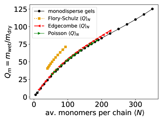
Figure 10: PB CGM prediction (for $f=0.5$, $c_{\mathrm{salt}}^{\mathrm{res}}=0.1$ mol/l, $\varepsilon_{\mathrm{r}}=80$): The figure shows the (mass-based) degree of swelling $Q_{m}$ as a function of the average chain length $\langle N\rangle$. In black the results for different monodisperse gels are shown. For the same charge fraction and reservoir salt concentration, the plot also shows the average mass-based degree of swelling $\langle Q_{m}\rangle_{N}$ for polydisperse gels (orange, red, green curves) plotted over the average chain length $\langle N\rangle_{N}$.

In figure 10 we compare the degree of swelling of monodisperse gels to polydisperse gels with the same average chain length. We find that the swelling of polydisperse gels highly depends on the chain length distribution. We observe an increased degree of swelling for polydisperse gels which have a geometric chain length distribution. The fact, that the introduced Flory-Schulz polydispersity increases the degree of swelling can be understood as an effect of the tail of the pmf: gels with longer chains swell more. Close to no increase in the degree of swelling is observed for a gel with a chain length distribution which is of Poisson type or follows the distribution by Edgecombe[35]. Since the Poisson distribution is rather sharp it is expected[71], and observed in our simple model, that the polydispersity has only little influence on the mass based degree of swelling. We want to emphasize that [35] reported a decrease in the swelling of his polydisperse gel model compared to the monodisperse gel in contrast to our approach. This difference could be a result of strong correlations in their gel model originating basically from the small unit cell they consider - inter chain correlations are overestimated. Additionally, it is not clear how different chain length heterogeneities like e.g. a Flory-Schulz distribution would impact the results reported by [35]. Representing a broad chain length distribution requires to simulate many chains in a unit cell, hence a huge computational effort. In contrast to the simulations of Edgecombe, our simplistic model for accounting chain length polydispersity lacks inter-chain correlations which seem to play an important role[65]. Measuring the correlations and accounting for them in simulations remains an open task for theorists as well as experimentalists[65]. We conclude that there is a discrepancy between the reported decrease in swelling by Edgecombe et al.   for polydisperse gels and the data shown in figure 10 for the chain length distribution of Edgecombe in our simple model. Our simplistic model for accounting chain length polydispersity lacks inter-chain correlations (in contrast to the simulations of Edgecombe). Therefore, correlations between the stretching state of different chains in the gel seem to play an important role[65]. Correlations and special topological conditions in the gel cannot be taken into account in our simple model of polydispersity since we assume independent chains. Measuring the correlations and accounting for them in simulations remains an open task for theorists as well as experimentalists[65]. Please note that a non-affine deformation of the gel alters the equilibrium volume which is predicted by equation (31). In the case of a non-affine deformation $A$ is a function of the end-to-end distance. Therefore, non-affine deformations of the gel alter the prediction of the mass-based degree of swelling for monodisperse gels, as well as for polydisperse gels.

5 Conclusion

In summary, we have presented two successive mean-field models aimed at describing gel swelling and the elastic moduli of polyelectrolyte gels: the single chain CGM and the Poisson-Boltzmann CGM. We find that the single chain CGM provides an excellent agreement with the periodic gel model. Since it is particle-based, we can use exactly the same interactions as in the periodic gel model, and hence also investigate specific ion effects (modeled via different short range interactions), poor solvent conditions, or the influence of multivalent ions. The single chain CGM provides about one order of magnitude reduction of the computational cost due to the smaller number of particles that need to be simulated. The PB CGM and the Katchalsky model provide several additional orders of magnitude in speed-up compared to the single chain model. On one hand, this speed-up comes at the cost of reduced accuracy. On the other hand, computationally cheaper models allow to screen the the possible parameter space, needed for optimizing real-world applications, more efficiently. While the Katchalsky model fails for charge fractions $f>0.5$, our new PB CGM still works for highly charged gels. In addition, both, the PB CGM and the single chain CGM, can be used to study pH-sensitive gels[37], where high charge fractions occur. The results for the bulk modulus of the single chain CGM and the PB CGM are consistent with periodic gel results (within errorbars).Additionally, we explore gel swelling as a function of solvent permittivity. For large relative permittivities the ideal Donnan prediction is recovered, while for lower relative permittivities electrostatic correlations lead to the expected deviations between the PB CGM and the periodic gel model. Nevertheless, our single chain CGM can still capture these correlation effects correctly. In addition, we demonstrated a simplistic approach of introducing chain length heterogeneity by assuming a mean-field factorization of the gel into uncorrelated single chain cells.

6 Acknowledgments

Funding from the German Research Foundation (DFG) through grants HO 1108/26-1, 423435431 (HO1108/30-1) as part of FOR 2811, and AR 593/7-1 is gratefully acknowledged. We thank D. Sean, K. Szuttor, P. Kreissl and J. Zeman for helpful discussions.

7 Supplementary Information

7.1 Influence of the Different Imposed Charge Densities in the PB CGM

We now investigate the influence of the imposed charge densities in the PB CGM and exchange the rectangular monomer density with an approximately Gaussian monomer density with compact support. The choice of the monomer density affects the charge density $\rho_{f}$ which is input to the PB equation.

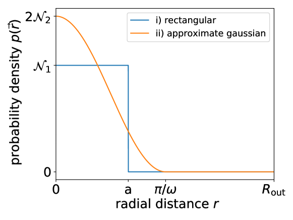
Figure 11: Different probability densities to find a monomer in distance $r$ from the end-to-end vector which are used in the PB CGM. The figure shows i) the rectangular probability density and ii) the approximately Gaussian probability density.

If the probability density to find a monomer in a given distance $r$ from the end-to-end vector is approximately Gaussian, then it is given via the following formula:

$$p(\vec{r})=\mathcal{N}_{2}(1+\cos(\omega r))H(-(r-\pi/\omega)).$$ (30)

$\mathcal{N}_{2}$ is a normalization constant such that $p(\vec{r})$ is a probability density ($\int_{V_{\mathrm{chain}}}\mathrm{d}Vp(\vec{r})=2\pi L\int_{0}^{R}\mathrm{d}rrp(\vec{r})=1$). This normalization criterion yields $\mathcal{N}_{2}=\frac{2\omega^{2}}{-4+\pi^{2}}\frac{1}{2\pi L}$. The parameter $\omega$ is chosen such that $\langle r\rangle\overset{!}{=}\langle r\rangle_{\text{MD}}$ is matched to the average distance of the monomers from the end-to-end vector. This condition yields $\omega=\frac{2(-6\pi+\pi^{3})}{3(-4+\pi^{2})\langle r\rangle_{\text{MD}}}$ which determines the width of the probability density. A comparison between the approximately Gaussian probability density and the rectangular probability density to find a monomer in distance $r$ can be seen in figure 11.

Imposing this alternative monomer density and solving the PB CGM again for the resulting alternative choice of $\rho_{f}(\vec{r})=-Nfp(\vec{r})$. We obtain only marginally changed swelling equilibria (compared to the imposed rectangular monomer density). This fact is depicted in figure 12 which barely allows to distinguish the resulting swelling equilibria.

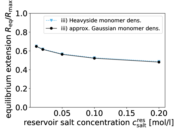
Figure 12: Comparison for different monomer densities (rectangular or approximate Gaussian density) in the PB model. The equilibrium swelling length $R_{\mathrm{eq}}$ as a function of the reservoir salt concentration $c_{\mathrm{salt}}^{\mathrm{res}}$ for $f=1$, $\varepsilon_{\mathrm{r}}=80$ and $N=40$.

7.2 Influence of the Different Imposed Values of $A$

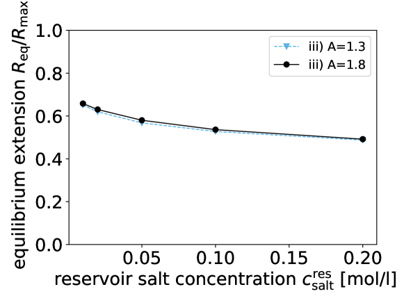
Figure 13: Comparison of different values of $A$ in the PB model (for the rectangular charge distribution). The equilibrium swelling length $R_{\mathrm{eq}}$ as a function of the reservoir salt concentration $c_{\mathrm{salt}}^{\mathrm{res}}$ for $f=1$, $\varepsilon_{\mathrm{r}}=80$ and $N=40$.

Košovan et al. [29] investigated the relation between the end-to-end distance and the volume per chain. They found (their figure 10) in MD simulations of periodic gels that the ratio $A=R_{\mathrm{e}}^{3}/V_{\mathrm{chain}}$ varies between roughly 1.8 and 1.5 and depends on the compression state of the gel, the charge fraction of the gel and the salt concentration of the reservoir. This fact is in contrast to our two new models where $A={\sqrt{27}}/{4}\approx 1.3$ is fixed. The easiest approach to test the influence of $A$ on our models is to impose a value of $A=1.8$ and compare it to results where $A$ was chosen to be $\sqrt{27}/4$. The effect of a change of $A$ on the predicted swelling equilibria of the PB CGM can be seen in figure 13. We conclude that the value of the end-to-end distance $R_{\mathrm{eq}}$, predicted by the PB CGM, is not sensitive to a change of the exact value of the ratio $A$: The predicted swelling equilibria barely change on a change of $A$. However, the predicted volume per chain is quite sensitive to the value of $A$ through equation (31):

$$V_{\mathrm{chain}}\approx L(R_{\mathrm{e}})^{3}/A.$$ (31)

7.3 P-$R_{\mathrm{e}}$ curves

For completeness we show the P-$R_{\mathrm{e}}$ curves which were used in this paper for determining the swelling equilibria in the following figures.

7.4 Swelling equilibria

For completeness, we show the swelling equilibria as a function salt concentration $c_{\mathrm{salt}}^{\mathrm{res}}$, charge fraction $f$ and chain length $N$. The plots are analogous to the plots in figure 3. For parameters where the Katchalsky model predicts more than one zero crossing in the $PV$ curve, the corresponding value of $R_{\mathrm{eq}}$ is set to zero (in order to indicate failure).

7.4.1 Salt Concentration Dependence

7.4.2 Charge Fraction Dependence

7.4.3 Chain Length Dependence

7.5 Comparison of the Models to the Periodic Gel Model

We compare the swelling predictions of the two CGMs and the Katchalsky model to the periodic gel model predictions in a parametric plot (similar to figure 5 in the main article). We seperately show the data for two data sets A: ($N=40,f=0.125$, $c_{\mathrm{salt}}^{\mathrm{res}}\in$ {0.01, 0.02, 0.05, 0.1, 0.2} mol/l) and B: ($N=80,f=1$, $c_{\mathrm{salt}}^{\mathrm{res}}\in$ {0.01, 0.02, 0.05, 0.1, 0.2} mol/l) in figures 14(a) and 14(b).

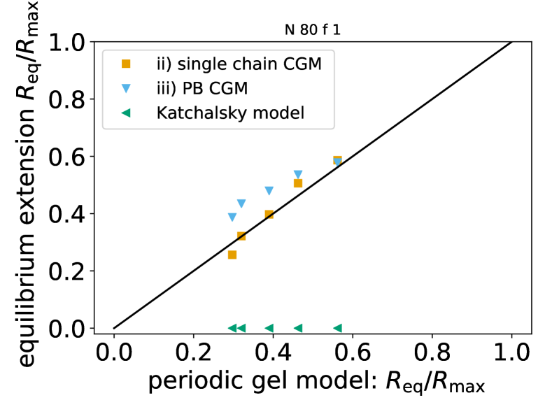
(a)

(b)

Figure 14: a) Data set A: N=40, f=0.125, different salt concentrations. b) Data set B: N=80, f=1, different salt concentrations. In each figure the highest salt concentration 0.2 mol/l is associated with the lowest swelling. Reducing the salt concentration increases the swelling. The Katchalsky model fails for f=1. To illustrate this failure, we set the predicted swelling to $R_{\mathrm{eq}}/R_{\mathrm{max}}=0$.

Plotting both data sets A and B together, like we do it in figure 5 of the article gives figure 15 below:

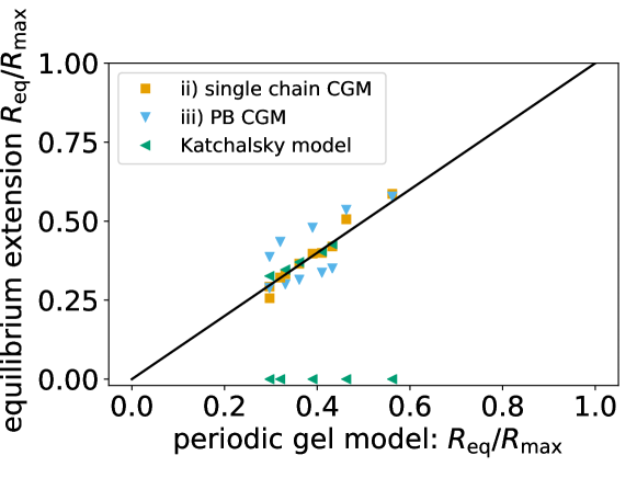
Figure 15: Data sets A and B from figures 14(a) and 14(b) plotted together. This plot is similar to figure 5 in the manuscript but contains only 1/6 of the data sets.

The projection of the predictions from a three-dimensional parameter space on one abscissa results in an apparent “scattering” of data around the ideal prediction (although the models do not scatter when plotting one data set alone). This indicates that the different models perform differently well in different parts of the parameter space.

References

- [1] Johannes Höpfner, Tobias Richter, Peter Košovan, Christian Holm, and Manfred Wilhelm. Seawater desalination via hydrogels: Practical realisation and first coarse grained simulations. In Gabriele Sadowski and Walter Richtering, editors, Intelligent Hydrogels, volume 140 of Progress in Colloid and Polymer Science, pages 247–263. Springer International Publishing, 2013.
- [2] Tobias Richter, Jonas Landsgesell, Peter Košovan, and Christian Holm. On the efficiency of a hydrogel-based desalination cycle. Desalination, 414:28–34, 2017.
- [3] N. A. Peppas, P. Bures, W. Leobandung, and H. Ichikawa. Hydrogels in pharmaceutical formulations. European journal of pharmaceutics and biopharmaceutics, 50(1):27–46, 2000.
- [4] X. Jia and K. L. Kiick. Hybrid multicomponent hydrogels for tissue engineering. Macromolecular Bioscience, 9:140–156, 2009.
- [5] J. Jagur-Grodzinski. Polymeric gels and hydrogels for biomedical and pharmaceutical applications. Polymers for Advanced Technologies, 21:27–47, 2009.
- [6] Lukas Arens, Felix Weißenfeld, Christopher O Klein, Karin Schlag, and Manfred Wilhelm. Osmotic engine: Translating osmotic pressure into macroscopic mechanical force via poly (acrylic acid) based hydrogels. Advanced Science, 4(9):1700112, 2017.
- [7] M. J. Zohuriaan-Mehr, H. Omidian, S. Doroudiani, and K. Kabiri. Advances in non-hygienic applications of superabsorbent hydrogel materials. Journal of Materials Science, 45(21):5711–5735, November 2010.
- [8] KS Kazanskii and SA Dubrovskii. Chemistry and physics of agricultural hydrogels. In Polyelectrolytes Hydrogels Chromatographic Materials. Advances in Polymer Science, volume 104, pages 97–133. Springer Verlag, 1992.
- [9] P. J. Flory and J. Rehner. Statistical mechanics of crosslinked polymer networks i. rubberlike elasticity. Journal of Chemical Physics, 11:512, 1943.
- [10] A. Katchalsky and I. Michaeli. Polyelectrolyte gels in salt solutions. Journal of Polymer Science, 15:69, 1955.
- [11] J. Ricka and Toyoichi Tanaka. Swelling of ionic gels: quantitative performance of the donnan theory. Macromolecules, 17(12):2916–2921, 1984.
- [12] A. R. Khokhlov, S. G. Starodubtzev, and V.. V. Vasilevskaya. Responsive gels: Volume transitions I. In K. Dušek, editor, Conformational transitions in polymer gels: theory and experiment, volume 109 of Adv. Polym. Sci., page 123. Springer Verlag, New York, 1993.
- [13] M. Rubinstein, R. H. Colby, A. V. Dobrynin, and J. F. Joanny. Elastic moduluS and equilibrium swelling of polyelectrolyte gels. Macromolecules, 29(1):398–406, 1996.
- [14] Gil C. Claudio, Kurt Kremer, and Christian Holm. Comparison of a hydrogel model to the poisson-boltzmann cell model. The Journal of Chemical Physics, 131(9):094903, September 2009.
- [15] Gabriel S. Longo, Monica Olvera de la Cruz, and I. Szleifer. Molecular theory of weak polyelectrolyte gels: The role of pH and salt concentration. Macromolecules, 44:147–158, 2011.
- [16] Manuel Quesada-Pérez, Jose Alberto Maroto-Centeno, Jacqueline Forcada, and Roque Hidalgo-Alvarez. Gel swelling theories: the classical formalism and recent approaches. Soft Matter, 7:10536–10547, 2011.
- [17] Prateek K. Jha, Jos W. Zwanikken, Juan J. de Pablo, and Monica Olvera de la Cruz. Electrostatic control of nanoscale phase behavior of polyelectrolyte networks. Current Opinion in Solid State and Materials Science, 15(6):271 – 276, 2011. Functional Gels and Membranes.
- [18] Andrea J Liu, Gary S Grest, M Cristina Marchetti, Gregory M Grason, Mark O Robbins, Glenn H Fredrickson, Michael Rubinstein, and Monica Olvera de la Cruz. Opportunities in theoretical and computational polymeric materials and soft matter. Soft Matter, 11(12):2326–2332, 2015.
- [19] Stefanie Schneider and Per Linse. Swelling of cross-linked polyelectrolyte gels. The European Physical Journal E, 8:457–460, 2002.
- [20] Quiliang Yan and Juan J. de Pablo. Monte carlo simulation of a coarse-grained model of polyelectrolyte networks. Physical Review Letters, 91(1):018301, July 2003.
- [21] Samuel Edgecombe, Stefanie Schneider, and Per Linse. Monte carlo simulations of defect-free cross-linked gels in the presence of salt. Macromolecules, 37(26):10089–10100, 2004.
- [22] De-Wei Yin, Qiliang Yan, and Juan J. de Pablo. Molecular dynamics simulation of discontinuous volume phase transitions in highly-charged crosslinked polyelectrolyte networks with explicit counterions in good solvent. The Journal of Chemical Physics, 123(17):174909, 2005.
- [23] Bernward A. Mann, Christian Holm, and Kurt Kremer. Swelling of polyelectrolyte networks. Journal of Chemical Physics, 122(15):154903, 2005.
- [24] Bernward A. Mann, Christian Holm, and Kurt Kremer. The swelling behaviour of charged hydrogels. Macromolecular Symposia, 237:90–107, 2006.
- [25] De-Wei Yin, Ferenc Horkay, Jack F. Douglas, and Juan J. de Pablo. Molecular simulation of the swelling of polyelectrolyte gels by monovalent and divalent counterions. Journal of Chemical Physics, 129(15), October 2008.
- [26] Bernward A. Mann, Olaf Lenz, Kurt Kremer, and Christian Holm. Hydrogels in poor solvents: A molecular dynamics study. Macromolecular Theory and Simulations, 20:721–734, 2011. Cover Issue.
- [27] Manuel Quesada-Pérez, Jose Guadalupe Ibarra-Armenta, and Alberto Martín-Molina. Computer simulations of thermo-shrinking polyelectrolyte gels. The Journal of Chemical Physics, 135(9):094109, 2011.
- [28] Peter Košovan, Tobias Richter, and Christian Holm. Molecular simulations of hydrogels. In Gabriele Sadowski and Walter Richtering, editors, Intelligent Hydrogels, volume 140 of Progress in Colloid and Polymer Science, pages 205–221. Springer International Publishing, 2013.
- [29] Peter Košovan, Tobias Richter, and Christian Holm. Modeling of polyelectrolyte gels in equilibrium with salt solutions. Macromolecules, 48(20):7698–7708, 2015.
- [30] Oleg Rud, Tobias Richter, Oleg Borisov, Christian Holm, and Peter Košovan. A self-consistent mean-field model for polyelectrolyte gels. Soft Matter, 13(18):3264–3274, 2017.
- [31] Thiago Colla, Christos N. Likos, and Yan Levin. Equilibrium properties of charged microgels: A poisson-boltzmann-flory approach. The Journal of Chemical Physics, 141(23), 2014.
- [32] Alan R. Denton and Qiyun Tang. Counterion-induced swelling of ionic microgels. The Journal of Chemical Physics, 145(16):164901, 2016.
- [33] AA Gavrilov and AV Chertovich. Computer simulation of random polymer networks: Structure and properties. Polymer Science Series A, 56(1):90–97, 2014.
- [34] Carsten Svaneborg, Gary S Grest, and Ralf Everaers. Disorder effects on the strain response of model polymer networks. Polymer, 46(12):4283–4295, 2005.
- [35] Samuel Edgecombe and Per Linse. Monte carlo simulation of polyelectrolyte gels: Effects of polydispersity and topological defect. Macromolecules, 40(10):3868–3875, May 2007.
- [36] Jonas Landsgesell, Lucie Nova, Oleg Rud, Filip Uhlik, David Sean, Pascal Hebbeker, Christian Holm, and Peter Košovan. Simulations of ionization equilibria in weak polyelectrolyte solutions and gels. Soft Matter, 15(6):1155–1185, 2019.
- [37] Jonas Landsgesell, David Sean, Patrick Kreissl, Kai Szuttor, and Christian Holm. Modeling gel swelling equilibrium in the mean field: From explicit to poisson-boltzmann models. Physical Review Letters, 122:208002, May 2019.
- [38] J-L. Barrat, J-F. Joanny, and P. Pincus. On the scattering properties of polyelectrolyte gels. Journal de Physique II, 2:1531–1544, 1992.
- [39] Florian Weik, Rudolf Weeber, Kai Szuttor, Konrad Breitsprecher, Joost de Graaf, Michael Kuron, Jonas Landsgesell, Henri Menke, David Sean, and Christian Holm. ESPResSo 4.0 – an extensible software package for simulating soft matter systems. The European Physical Journal Special Topics, 227(14):1789–1816, 2019.
- [40] J. D. Weeks, D. Chandler, and H. C. Andersen. Role of repulsive forces in determining the equilibrium structure of simple liquids. The Journal of Chemical Physics, 54:5237, 1971.
- [41] Kurt Kremer and Gary S. Grest. Dynamics of entangled linear polymer melts: A molecular-dynamics simulation. Journal of Chemical Physics, 92(8):5057–5086, 1990.
- [42] Gary S. Grest and Kurt Kremer. Molecular dynamics simulation for polymers in the presence of a heat bath. Physical Review A, 33(5):3628–31, 1986.
- [43] Markus Deserno and Christian Holm. How to mesh up Ewald sums. I. A theoretical and numerical comparison of various particle mesh routines. Journal of Chemical Physics, 109:7678, 1998.
- [44] Markus Deserno and Christian Holm. How to mesh up Ewald sums. II. An accurate error estimate for the Particle-Particle-Particle-Mesh algorithm. Journal of Chemical Physics, 109:7694, 1998.
- [45] T.L. Hill. An Introduction to Statistical Thermodynamics. Addison-Wesley series in chemistry. Dover Publications, 1986.
- [46] Daan Frenkel and Berend Smit. Understanding Molecular Simulation. Academic Press, San Diego, 2 edition, 2002.
- [47] U. Essmann, L. Perera, M. L. Berkowitz, T. Darden, H. Lee, and L. Pedersen. A smooth Particle Mesh Ewald method. Journal of Chemical Physics, 103:8577, 1995.
- [48] Dmytro Antypov and Christan Holm. Optimal cell approach to osmotic properties of finite stiff-chain polyelectrolytes. Physical Review Letters, 96:088302, 2006.
- [49] Axel Arnold and Christian Holm. MMM1D: A method for calculating electrostatic interactions in 1D periodic geometries. Journal of Chemical Physics, 123(12):144103, September 2005.
- [50] H. Wennerström, B. Jönsson, and P. Linse. The cell model for polyelectrolyte systems. exact statistical mechanical relations, monte carlo simulations, and the poisson–boltzmann approximation. Journal of Chemical Physics, 76:4665, 1982.
- [51] T. Alfrey, P. W. Berg, and H. J. Morawetz. The counterion distribution in solutions of rod-shaped polyelectrolyteS. Journal of Polymer Science, 7:543, 1951.
- [52] R. M. Fuoss, A. Katchalsky, and S. Lifson. The potential of an infinite rod-like molecule and the distribution of the counter ions. Proceedings of the National Academy of Sciences of the United States of America, 37:579–589, 1951.
- [53] Tomer Markovich, David Andelman, and Rudi Podgornik. Charged Membranes: Poisson-Boltzmann theory, DLVO paradigm and beyond, chapter 1. Taylor & Francis / CRC Press, 2016.
- [54] Emmanuel Trizac and J.-P Hansen. Wigner-seitz model of charged lamellar colloidal dispersions. Physical Review E, 56:3137, 1997.
- [55] TM Birshtein and Victor A Pryamitsyn. Coil-globule type transitions in polymers. 2. theory of coil-globule transition in linear macromolecules. Macromolecules, 24(7):1554–1560, 1991.
- [56] A Cohen. A padé approximant to the inverse langevin function. Rheologica acta, 30(3):270–273, 1991.
- [57] Michael Rubinstein and Ralph H. Colby. Polymer Physics. Oxford University Press, Oxford, UK, 2003.
- [58] David Andelman. Handbook of Biological Physics, chapter 12, page 603. School of Physics and Astronomy, Tel Aviv University, 1995.
- [59] Markus Deserno, Christian Holm, and Sylvio May. Fraction of condensed counterions around a charged rod: Comparison of Poisson-Boltzmann theory and computer simulations. Macromolecules, 33:199–206, 2000.
- [60] Bernward A. Mann, Ralf Everaers, Christian Holm, and Kurt Kremer. Scaling in polyelectrolyte networks. Europhysics Letters, 67(5):786–792, 2004.
- [61] Manuel Quesada-Pérez, Jose Ramos, Jacqueline Forcada, and Alberto Martín-Molina. Computer simulations of thermo-sensitive microgels: Quantitative comparison with experimental swelling data. The Journal of Chemical Physics, 136(24):244903, 2012.
- [62] Manuel Quesada-Pérez, José Alberto Maroto-Centeno, and Alberto Martín-Molina. Effect of the counterion valence on the behavior of thermo-sensitive gels and microgels: A monte carlo simulation study. Macromolecules, 45(21):8872–8879, 2012.
- [63] W. Hummel, U. Berner, E. Curti, F.J. Pearson, and T. Thoenen. Nagra/PSI Chemical Thermodynamic Data Base 01/01. Universal Publishers, 2002.
- [64] Tobias Richter. Coarse grained Hydrogels. PhD thesis, 2017.
- [65] Chase P Broedersz and Fred C MacKintosh. Modeling semiflexible polymer networks. Reviews of Modern Physics, 86(3):995, 2014.
- [66] Wolfgang Demtröder. Experimentalphysik 1: Mechanik und Wärme. Springer-Verlag Berlin, Heidelberg, New York, 2004.
- [67] Ali Naji and Roland R Netz. Scaling and universality in the counterion-condensation transition at charged cylinders. Physical Review E, 73(5):056105, 2006.
- [68] S. Schneider and P. Linse. Discontinuous volume transitions in cross-linked polyelectrolyte gels induced by short-range attractions and strong electrostatic coupling. Macromolecules, 37:3850–3856, 2004.
- [69] Sergei Panyukov and Yitzhak Rabin. Statistical physics of polymer gels. Physics Reports, 269(1–2):1–131, 1996.
- [70] Mohammad Tehrani, Mohammad Hossein Moshaei, and Alireza S Sarvestani. Network polydispersity and deformation-induced damage in filled elastomers. Macromolecular Theory and Simulations, 26(6):1700038, 2017.
- [71] Gert Strobl. The Physics of Polymers. Springer, 3 edition, 2007.
- [72] Paul J Flory. Molecular size distribution in linear condensation polymers1. Journal of the American Chemical Society, 58(10):1877–1885, 1936.
- [73] McNaught and Wilkinson. IUPAC. Compendium of Chemical Terminology, 2nd ed. (the "Gold Book"). 1997.