On volume subregion complexity in Vaidya spacetime

Roberto Auzzi^a,b, Giuseppe Nardelli^a,c,

Fidel I. Schaposnik Massolo^d, Gianni Tallarita^e, Nicolò Zenoni^a,b,f

^a Dipartimento di Matematica e Fisica, Università Cattolica del Sacro Cuore,
Via Musei 41, 25121 Brescia, Italy

^b INFN Sezione di Perugia, Via A. Pascoli, 06123 Perugia, Italy

^c TIFPA - INFN, c/o Dipartimento di Fisica, Università di Trento,
38123 Povo (TN), Italy

^d Institut des Hautes Études Scientifiques,
35 route de Chartres, 91440 Bures-sur-Yvette, France

^e Departamento de Ciencias, Facultad de Artes Liberales, Universidad Adolfo Ibáñez, Santiago 7941169, Chile,

^f Instituut voor Theoretische Fysica, KU Leuven, Celestijnenlaan 200D, B-3001 Leuven, Belgium

E-mails: roberto.auzzi@unicatt.it, giuseppe.nardelli@unicatt.it, fidels@ihes.fr, gianni.tallarita@uai.cl, nicolo.zenoni@unicatt.it

We study holographic subregion volume complexity for a line segment in the AdS₃ Vaidya geometry. On the field theory side, this gravity background corresponds to a sudden quench which leads to the thermalization of the strongly-coupled dual conformal field theory. We find the time-dependent extremal volume surface by numerically solving a partial differential equation with boundary condition given by the Hubeny-Rangamani-Takayanagi surface, and we use this solution to compute holographic subregion complexity as a function of time. Approximate analytical expressions valid at early and at late times are derived.

1 Introduction

In the AdS/CFT correspondence, quantum information concepts such as entanglement entropy have simple geometrical descriptions, e.g. the area of a minimal surface in the bulk gravity dual [1, 2, 3]. These results put on a more general picture the idea that the area of the event horizon is proportional to the black hole entropy [4]. It is then reasonable that more sophisticated quantum information physical quantities computed on the boundary theory may give us further insights on how other geometrical properties of the bulk dual may be reconstructed from the boundary.

Recently, a new quantum information concept has been introduced in order to describe the growth of the Einstein-Rosen Bridge (ERB) inside the horizon of a black hole, which continues for a much longer time than the thermalization time. Entanglement entropy is not enough to describe the dynamics behind the event horizon and the late-time evolution of the wormhole interior, because it approaches the equilibrium on a time scale which is of the same order as the thermalization time scale. It has been suggested that the relevant quantity in the dual field theory is quantum computational complexity [5, 6, 7]. This is heuristically defined as the minimal number of elementary unitary operations that are required in order to prepare a given state from a reference one. In quantum mechanics, a geometrical approach to complexity was developed by Nielsen and collaborators [8, 9]. In Quantum Field Theory (QFT), a rigorous definition of complexity involves several subtleties, see e.g. [10, 11, 12, 13, 14, 15] for attempts to define it more rigorously.

Two holographic quantities have been conjectured to be the gravity dual of complexity:

• Complexity=Volume (CV) conjecture: complexity is proportional to the volume of extremal space-like slices [5, 6, 7];

• Complexity=Action (CA) conjecture: complexity is proportional to the action evaluated on the Wheeler-deWitt (WdW) patch [16, 17]. It is interesting that a proper action calculation involves null boundaries and joint terms that have been recently studied in [18].

Both conjectures have been recently investigated by several groups in many physical settings, e.g. [19, 20, 21, 22, 23, 24, 25, 26, 27, 28, 29]. One interesting situation is the global quench, which can be represented in AdS/CFT by the Vaidya geometry, see e.g. [30]. Holographic complexity in these geometries was previously studied in [31, 32, 33, 34]. Another interesting situation is the local quench [35], whose complexity was studied in [36, 37].

Quantum states localised on a subregion on the boundary should be dual to the entanglement wedge [38, 39]. Consequently, it is natural to conjecture that the complexity of a mixed state (which should be properly defined) is dual to some version of the holographic CV or CA conjecture, adapted to the corresponding subregion [40, 41].

For the CV proposal, it is natural to conjecture [40] that such mixed state complexity is dual to the extremal volume of the region $\gamma$ delimited by the boundary subregion on which the mixed state is localised and its Hubeny-Rangamani-Takayanagi (HRT) [42] surface, whose area corresponds to the holographic entanglement entropy, i.e.

$$C_{V}=\max_{\gamma}\frac{V(\gamma)}{GL_{AdS}}\,,$$ (1.1)

where $G$ is the Newton constant and $L_{AdS}$ the AdS length scale. Concerning the CA conjecture, a proposal involving the action defined on a region $\Sigma$ which is the intersection of the entanglement wedge and of the WdW patch has been introduced in [41],

$$C_{A}=\frac{I_{\Sigma}}{\pi\hbar}\ .$$ (1.2)

In both cases, the precise nature of the conjectured notion of mixed state complexity is still unknown and several proposals have been put forward, see e.g. [40, 43, 44]. Other studies on subregion complexity include [45, 46, 47, 48, 49, 50, 51, 52, 53].

In order to get insights on the possible field theory dual quantities, it is necessary to explicitly compute subregion complexity in several physical settings. The purpose of this paper is to study holographic subregion volume complexity, using the CV conjecture, for a line segment in the AdS₃ Vaidya spacetime. The study of subregion complexity in this physical situation was initiated in [54]. Moreover, the issue was studied also in modified gravity [55, 56]. In all these previous works, an ansatz in which the extremal volume is taken independent of the spatial coordinate $x$ is used. This is correct in the case of time-independent geometries; however we find that this ansatz is not consistent with the boundary condition given by the HRT surface for the Vaidya geometry. In this paper we determine the extremal surface numerically and we find that the $x$-independent ansatz is in general a good approximation only at early and late times. In the case of small subregion size $l\ll 1/T$, where $T$ is the temperature, the $x$-independent ansatz provides a good approximation also at intermediate times.

The paper is organised as follows: in section 2 we review the analytic solution for the HRT surfaces in case of zero thickness shell. In section 3 we show that the $x$-independent ansatz is not consistent for the extremal volume in the time-dependent case and we compute the $x$-dependent solution and its volume numerically. We conclude in section 4. Some technical details are collected in appendices.

Note added: After this work was finished and the present paper was in the writing stage, Ref. [57] was submitted on arXiv. Our approximate analytical results agree with them in the early time regime. At intermediate times, we expect that the $x$-independent ansatz used in [57] is not accurate.

2 Space-like geodesics

We study the Complexity=Volume conjecture for subregions in AdS₃ Vaidya spacetime. In three dimensions, the HRT surface attached to a segment coincides with a space-like geodesic. Here we review some basic aspects of these geodesics following [30], which studies the thermalization of the entanglement entropy in detail. We use interchangeably $r$ or $z=1/r$ as a radial AdS coordinate. The spacetime metric is

$$ds^{2} = -r^{2}f(v,r)\,dv^{2}+2\,dv\,dr+r^{2}\,dx^{2}$$ (2.1)

$$= \frac{1}{z^{2}}\left[-f\left(v,z\right)dv^{2}-2\,dv\,dz+dx^{2}\right]\,,$$

where we have fixed the AdS radius $L_{AdS}=1$ and

$$f=1-\frac{m(v)}{r^{2}}=1-m(v)\,z^{2}\,.$$ (2.2)

The $v$ coordinate is constant along infalling null rays and it coincides with the time coordinate $t$ on the spacetime boundary, located at $r\rightarrow\infty$ (or, equivalently, at $z\rightarrow 0$). For constant $m(v)$, changing variables to $t$, with $dv=dt-\frac{dz}{f}$, the solution is the Banados-Teitelboim-Zanelli (BTZ) [58, 59] black hole in Schwarzschild coordinates:

$$ds^{2}=\frac{1}{z^{2}}\left(-fdt^{2}+\frac{dz^{2}}{f}+dx^{2}\right)\,.$$ (2.3)

We will be interested in the case in which the function $m(v)$ models a field theory quench, i.e. it interpolates between $m=0$ and $m=M$.

For concreteness, in the numerical calculations we will consider the choice

$$\qquad m(v)=\frac{M}{2}\left(1+\tanh\frac{v}{\tilde{v}}\right)\,,$$ (2.4)

where $M$ is proportional to the final BH mass and $\tilde{v}$ parameterizes the thickness of the shell. The $\tilde{v}\rightarrow 0$ limit corresponds to zero thickness; in this case $m(v)$ can be written in terms of the Heaviside step function $\vartheta$:

$$m(v)=M\,\vartheta(v)\,.$$ (2.5)

In the zero thickness limit, analytical expressions for the geodesics are available. With the choice (2.5), the geometry described by eq. (2.1) is the AdS₃ one for $v<0$ and the BTZ black hole [58, 59] one for $v>0$. The BTZ black hole is formed by the gravitational collapse of a shell of null dust (here described by $v=0$) with infinitesimal thickness falling from the spacetime boundary.

Our purpose is to evaluate the subregion complexity of a boundary subregion. According to the CV conjecture for subregions, we have to compute the volume of an extremal codimension-one bulk surface delimited by the boundary subregion and the corresponding codimension-two HRT [42] surface. In the $2+1$ dimensional case, the $1$-dimensional HRT surface is a space-like geodesic anchored at the edges of the boundary subregion.

We consider as a subregion a segment of length $l$ lying on a constant time slice $t$ on the boundary, described by $x\in\left[-\frac{l}{2},\frac{l}{2}\right]$. The HRT surface can be parameterized as $v(x)$ and $r(x)$. The boundary conditions at $r=\infty$ are

$$x(r=\infty)=\pm\frac{l}{2}\,,\qquad v(r=\infty)=t\,.$$ (2.6)

By symmetry, the turning point is at $x=0$, i.e.

$$x(r=r_{*})=0\,,\qquad v(r=r_{*})=v_{*}\,,$$ (2.7)

where $r_{*}$ denotes the value of $r$ at the turning point. Note that both $r_{*}$ and $v_{*}$ are functions of the geodesic boundary condition $t$.

Since the spacetime is described by an AdS₃ part and a BTZ black hole portion glued at $v=0$, the HRT surface is given by the junction at $v=0$ of the HRT surface for a BTZ spacetime and the one for AdS₃ spacetime. In the following we denote with $r=r_{s}$ the position of this junction on the $v=0$ infalling null ray.

2.1 AdS₃ geodesics

For $v<0$, the Vaidya spacetime is AdS₃:

$$ds^{2}=-r^{2}dv^{2}+2\,dv\,dr+r^{2}\,dx^{2}\ .$$ (2.8)

The corresponding portion of the HRT surface is given by the equal-time space-like geodesic in the AdS geometry:

$$x_{\pm}(r)=\pm\frac{\sqrt{r^{2}-r_{*}^{2}}}{r_{*}r}\,,\qquad v_{\pm}(r)=\frac{1}{r_{s}}-\frac{1}{r}\,,$$ (2.9)

where $(r_{*},r_{s})$ are functions of the boundary time $t$ and of the length $l$. We will denote $\left(x_{+}(r),v_{+}(r)\right)$ and $\left(x_{-}(r),v_{-}(r)\right)$ as branches 1 and 2 of the geodesic, respectively. At initial time $t=0$, the geodesic is entirely in AdS and

$$r_{*}(t=0)=\frac{2}{l}\,.$$ (2.10)

2.2 BTZ geodesics

For $v>0$, the Vaidya spacetime is a BTZ black hole:

$$ds^{2}=-r^{2}\left(1-\frac{r_{h}^{2}}{r^{2}}\right)dv^{2}+2\,dv\,dr+r^{2}\,dx^{2}\ .$$ (2.11)

The event horizon of the black hole is located at $r=r_{h}$ and the Hawking temperature is $T=\frac{r_{h}}{2\pi}$.

The part of the HRT surface in the Vaidya spacetime for $v>0$ is given by the space-like geodesic in the BTZ geometry [30]:

$$x_{\pm}(r)=\frac{1}{4r_{h}}\left\{2\ln\left|\frac{r^{2}-J\,r_{h}^{2}\pm\sqrt{r^{4}+\left(E^{2}-J^{2}-1\right)r_{h}^{2}\,r^{2}+J^{2}\,r_{h}^{4}}}{r^{2}+J\,r_{h}^{2}\pm\sqrt{r^{4}+\left(E^{2}-J^{2}-1\right)r_{h}^{2}\,r^{2}+J^{2}\,r_{h}^{4}}}\right|+\ln\left|\frac{(J+1)^{2}-E^{2}}{(J-1)^{2}-E^{2}}\right|\right\}\,,$$ (2.12)

$$v_{\pm}(r)=t+\frac{1}{2r_{h}}\ln\left|\frac{r-r_{h}}{r+r_{h}}\ \frac{r^{2}-\left(E+1\right)r_{h}^{2}\pm\sqrt{r^{4}+\left(E^{2}-J^{2}-1\right)r_{h}^{2}\,r^{2}+J^{2}\,r_{h}^{4}}}{r^{2}+\left(E-1\right)r_{h}^{2}\pm\sqrt{r^{4}+\left(E^{2}-J^{2}-1\right)r_{h}^{2}\,r^{2}+J^{2}\,r_{h}^{4}}}\right|\,,$$ (2.13)

with $E$ and $J$ being two integration constants arising from the equations of motion (see appendix A). Depending on the values of $E,J$ in (2.12), (2.13), the structure of the geodesic changes; it is useful to distinguish four regions [30], see Fig. 1. In our notation, we have translated the solutions in $x$ in such a way that they are symmetric under the exchange $x\rightarrow-x$.

Figure 1: Kinds of space-like geodesics as function of $(J,E)$.

Let us start for simplicity with $E=0$, which corresponds to geodesics lying on $t$-constant slices. By symmetry, it is not restrictive to choose $J>0$ and then there are only two kinds of such geodesics (see Fig. 1): the ones with $J>1$ (region $I$) and the ones with $J<1$ (region $III$). In Fig. 2 we show the plot of the geodesic (2.12) for both the cases $J>1$ and $J<1$. By direct calculation, we find that the minimal value of $r$ along the geodesic is:

$$r_{0}=\begin{cases}J\,r_{h}\,,\qquad J>1\\ r_{h}\,,\qquad\,\,\,\,J<1\,.\\ \end{cases}$$ (2.14)

The geodesics relevant as HRT surfaces for the static BTZ black hole are the ones in region $I$, because they have minimal length compared to the ones in region $III$. Note that a space-like geodesic with $E=0$ in a static BTZ spacetime never penetrates inside the black hole. For $J>1$, the relation between the parameter $J$ and the spatial separation $l$ between the anchoring points of the geodesic is given by:

$$\frac{l}{2}=\frac{1}{4r_{h}}\ln\left(\frac{J+1}{J-1}\right)^{2}\,,\qquad{\rm or}\qquad J=\coth\left(\frac{r_{h}\,l}{2}\right)\,.$$ (2.15)

This allows to express $r_{0}$ as a function of the boundary separation $l$ in the $J>1$ case:

$$r_{0}=r_{h}\coth\left(\frac{r_{h}\,l}{2}\right)\ .$$ (2.16)

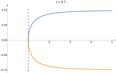
Figure 2: Plots of the space-like geodesic (2.12) in BTZ spacetime with $E=0$ and different values of the parameter $J$, with $r_{h}=1$. The blue curve represents $x_{+}(r)$, while the yellow one represents $x_{-}(r)$.

For generic $E$, there are in principle four different kinds of geodesics, one kind for each region of the $(E,J)$ plane in Fig. 1. In Fig. 3 we show a plot of (2.12) for each kind of geodesic. For $E\neq 0$, these geodesics connect points on the boundary with different values of $t$. Note that the geodesic on the bottom left of Fig. 3 penetrates inside the black hole, while this never happens for geodesics at constant $t$.

(I)	(II)
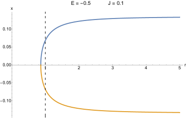
(III)	(IV)

Figure 3: Plots of the space-like geodesic (2.12) in BTZ spacetime with different values of the parameters $(E,J)$, with $r_{h}=1$. The blue curve represents $x_{+}(r)$, while the yellow one represents $x_{-}(r)$.

2.3 Joining the geodesics

The HRT surface in the full Vaidya spacetime can be obtained by gluing together the AdS₃ geodesic (2.9) and the BTZ one (2.12, 2.13) at $r=r_{s}$. Using the "refraction-like" law in [30], we can fix the two constants of motion of the BTZ portion of the geodesic:

$$E=-\frac{r_{h}\sqrt{r_{s}^{2}-r_{*}^{2}}}{2r_{s}^{2}}\,,\qquad J=\frac{r_{*}}{r_{h}}\,.$$ (2.17)

It is important to note that $E,J$ all depend on the boundary time $t$ and on the length $l$. Let us denote by $r_{m}$ the minimal value of the $r$-coordinate of the BTZ portion. If $r_{s}\geq r_{h}/\sqrt{2}$ we have to consider only branch 1, while if $r_{s}\leq r_{h}/\sqrt{2}$ also branch 2 comes into play. In the latter case, a part of branch 2 (with $r_{m}\leq r\leq r_{s}$) connects the AdS₃ geodesic and the full branch 1, which is anchored at the spacetime boundary.

It is useful to define:

$$\nu^{\pm}(r) = t+\frac{1}{2r_{h}}\ln\left|\frac{r-r_{h}}{r+r_{h}}\ \frac{r^{2}-\left(E+1\right)r_{h}^{2}\pm\sqrt{r^{4}+\left(E^{2}-J^{2}-1\right)r_{h}^{2}\,r^{2}+J^{2}\,r_{h}^{4}}}{r^{2}+\left(E-1\right)r_{h}^{2}\pm\sqrt{r^{4}+\left(E^{2}-J^{2}-1\right)r_{h}^{2}\,r^{2}+J^{2}\,r_{h}^{4}}}\right|\,,$$

$$\chi^{\pm}(r) = \left(\frac{1}{2r_{h}}\ln\left|\frac{r^{2}-J\,r_{h}^{2}\pm\sqrt{r^{4}+\left(-1+E^{2}-J^{2}\right)r_{h}^{2}\,r^{2}+J^{2}\,r_{h}^{4}}}{r^{2}+J\,r_{h}^{2}\pm\sqrt{r^{4}+\left(-1+E^{2}-J^{2}\right)r_{h}^{2}\,r^{2}+J^{2}\,r_{h}^{4}}}\right|+\frac{l}{2}\right)\,,$$ (2.18)

in which the values of $E$ and $J$ are given by eq. (2.17); for fixed length $l$, we must obey the following constraint for the quantities $(r_{s},r_{*})$:

$$0=2\frac{\sqrt{r_{s}^{2}-r_{*}^{2}}}{r_{s}\,r_{*}}+\frac{1}{r_{h}}\ln\frac{2r_{s}\left(r_{s}^{2}+r_{*}\,r_{h}\right)+\left(2r_{s}^{2}-r_{h}^{2}\right)\sqrt{r_{s}^{2}-r_{*}^{2}}}{2r_{s}\left(r_{s}^{2}-r_{*}\,r_{h}\right)+\left(2r_{s}^{2}-r_{h}^{2}\right)\sqrt{r_{s}^{2}-r_{*}^{2}}}-l=f_{l}(r_{s},r_{*})\,.$$ (2.19)

We can now build the total Vaidya geodesic by suitably glueing BTZ and AdS portions. In the case $r_{s}\geq\frac{r_{h}}{\sqrt{2}}$, the total geodesic is given by:

$$\hat{x}_{\pm}(r) = \begin{cases}\pm\frac{\sqrt{r^{2}-r_{*}^{2}}}{r_{*}\,r}&{\rm if}\quad r\leq r_{s},\,\,v\leq 0\\ \pm\chi^{+}(r)&{\rm if}\quad r>r_{s},\,\,v>0\,,\end{cases}$$

$$\hat{v}_{\pm}(r) = \begin{cases}\frac{1}{r_{s}}-\frac{1}{r}&{\rm if}\quad r\leq r_{s},\,\,v\leq 0\\ \nu^{+}(r)&{\rm if}\quad r>r_{s},\,\,v>0\,.\end{cases}$$ (2.20)

Instead, in the case $r_{s}\leq\frac{r_{h}}{\sqrt{2}}$, the full geodesic is:

$$\hat{x}_{\pm}(r) = \begin{cases}\pm\frac{\sqrt{r^{2}-r_{*}^{2}}}{r_{*}\,r}&{\rm if}\quad r\leq r_{s},\,\,v\leq 0\\ \pm\chi^{+}(r)&{\rm if}\quad r\geq r_{m},\,\,v>0\\ \pm\chi^{-}(r)&{\rm if}\quad r_{m}\leq r<r_{s},\,\,v>0\,,\end{cases}$$

$$\hat{v}_{\pm}(r) = \begin{cases}\frac{1}{r_{s}}-\frac{1}{r}&{\rm if}\quad r\leq r_{s},\,\,v\leq 0\\ \nu^{+}(r)&{\rm if}\quad r\geq r_{m},\,\,v>0\\ \nu^{-}(r)&{\rm if}\quad r_{m}\leq r<r_{s},\,\,v>0\,.\end{cases}$$ (2.21)

The minimal value $r_{m}$ of the $r$-coordinate on the BTZ geodesic is

$$r_{m}^{2}=\frac{r_{h}^{2}}{2}\left(1-E^{2}+J^{2}+\sqrt{\left(1-E^{2}+J^{2}\right)^{2}-4J^{2}}\right)\,,$$ (2.22)

where $E,J$ are given by eq. (2.17).

Since the shell of null dust is at $v=0$, the time dependence of the junction point $r_{s}$ can be determined by imposing that $v(r_{s})=0$ in eq. (2.13):

$$\frac{r_{s}}{r_{h}}=\frac{1}{2}\left(\coth(r_{h}t)+\sqrt{\coth^{2}(r_{h}t)-\frac{2\sqrt{1-\frac{r_{*}^{2}}{r_{s}^{2}}}}{1+\sqrt{1-\frac{r_{*}^{2}}{r_{s}^{2}}}}}\,\right)\,.$$ (2.23)

The system of Eqs. (2.23) and (2.19) determine the time dependence of $r_{s}$ and $r_{*}$; unfortunately they cannot be solved in closed form.

Figure 4: The plots show $r_{s}$ (solid line) and $r_{*}$ (dashed line) as a function of the boundary time $t$. Here $r_{h}=1$, and we set $l=5$ on the left and $l=12$ on the right.

In Fig. 4 we show numerical results for particular values of the boundary subregion size. At $t=0$ the HRT surface entirely lies in the AdS part of the full spacetime, and so $r_{s}\rightarrow\infty$ and $r_{*}(0)=2/l$. The thermalization time $t_{*}$ is given by the value of the boundary time at which $r_{s}$ and $r_{*}$ intersect. For $t>t_{*}$ the HRT surface entirely lies in the BTZ part of the dynamical spacetime; from this time the subregion complexity drops to the constant thermal value. Eqs. (2.23) and (2.19) give

$$t_{*}=l/2\,,\qquad r_{*}(t_{*})=r_{s}(t_{*})=r_{0}\,,$$ (2.24)

see (2.16). For $l\gg 1/r_{h}$, we have $r_{0}\rightarrow r_{h}$.

An example of the time evolution of the geodesics is shown in Fig. 5.

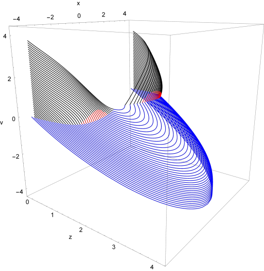
Figure 5: Time evolution of the geodesic for $l=8,r_{h}=1$. The black and red curves respectively denote branch 1 and 2 in the BTZ part; the blue curves denote the AdS part of the full geodesic.

2.4 Numerical geodesics

In order to solve the partial differential equations for the extremal volume, it is useful to consider the case of non zero $\tilde{v}$ in eq. (2.4) in order to make the numerical problem more tractable. For generic $\tilde{v}$, one has to solve the geodesics equations numerically:

$$\ddot{v}+\frac{\dot{v}^{2}}{z}-\frac{\dot{x}^{2}}{z}=0\,,\qquad\ddot{x}-2\frac{\dot{x}\dot{z}}{z}=0\,,$$

$$\ddot{z}+\left(z\,m(v)-\frac{2+z^{3}m^{\prime}(v)}{2z}\right)\dot{v}^{2}-\frac{2}{z}\dot{z}^{2}-\frac{2}{z}\dot{z}\dot{v}+\left(\frac{1}{z}-zm(v)\right)\dot{x}^{2}=0\,,$$ (2.25)

where the dot denotes a derivative with respect to the affine parameter $\lambda$ and the ^′ represents a derivative with respect to the coordinate $v$. The equations are solved with the boundary conditions shown in (2.6) using a shooting method implemented in Mathematica. In the $\tilde{v}\rightarrow 0$ limit, we recover the analytical solution in section 2.3.

3 Volume

In this section we compute the extremal volume of the region delimited by the segment of length $l$ and the HRT surface as a function of the boundary time $t$. This volume has been proposed to be dual to mixed state complexity in the boundary CFT [40].

3.1 Volume for AdS and BTZ

In the initial stage ($t\leq 0$) the volume of the region of interest is entirely in AdS₃, while at final time $t\geq l/2$ the volume is entirely in the BTZ geometry. So these cases correspond to the initial and final values of the subregion complexity. Moreover, the volume is ultraviolet divergent and a natural regularization is given by subtracting the initial AdS volume $V_{AdS}$. In this case the boundary geodesic is

$$x^{2}+z^{2}=(l/2)^{2}\,,$$ (3.1)

and the extremal volume solution is given by

$$z=t-v\,.$$ (3.2)

Introducing an UV cutoff at $z=1/\Lambda$, the AdS volume is

$$V_{AdS}=2\int_{1/\Lambda}^{l/2}\frac{\sqrt{(l/2)^{2}-z^{2}}}{z^{2}}dz=l\,\Lambda-\pi\,.$$ (3.3)

The volume at the final equilibrium time turns out to be exactly the same, i.e.

$$V_{BTZ}=V_{AdS}\,.$$ (3.4)

This non-trivial property holds only in AdS₃ and has topological roots: it can be proved using the Gauss-Bonnet theorem [46].

3.2 Inconsistency of the $x$-independent ansatz

Let us parameterise the volume by a surface $v(x,r)$ in AdS₃ Vaidya spacetime. The volume functional can be written as:

$$V=\int\,dr\,dx\,\mathcal{V}\,,\qquad\mathcal{V}=\sqrt{r^{2}(2-r^{2}f\partial_{r}v)\partial_{r}v-(\partial_{x}v)^{2}}\,,$$ (3.5)

where $f$ is a function only of $r,v$, and let us denote

$$v_{x}=\partial_{x}v\,,\qquad v_{r}=\partial_{r}v\,.$$ (3.6)

The Euler-Lagrange equation gives

$$\partial_{x}\left(\frac{\partial\mathcal{V}}{\partial v_{x}}\right)+\partial_{r}\left(\frac{\partial\mathcal{V}}{\partial v_{r}}\right)-\frac{\partial\mathcal{V}}{\partial v}=0\,.$$ (3.7)

Since the functional (3.5) is invariant by translations in $x$, it is reasonable to look for solutions of eq. (3.7) which are $x$-independent, i.e.

$$v_{x}=0\,,\qquad\partial_{x}v_{r}=0\,.$$ (3.8)

With the ansatz (3.8), and with the choice $f=f(r)=f_{BTZ}$, the equation of motion (3.7) reduces to an ordinary differential equation:

$$\left(3r_{h}^{2}-6r^{2}\right)v^{\prime}(r)^{2}+\left(-3r^{2}r_{h}^{2}+r_{h}^{4}+2r^{4}\right)v^{\prime}(r)^{3}-rv^{\prime\prime}(r)+2v^{\prime}(r)=0\,,$$ (3.9)

where the ^′ denotes a derivative with respect to the coordinate $r$.

The extremal surface used to compute the subregion complexity of a segment must be attached to the HRT surface, which in our case is a geodesic. Consequently, in order for the $x$-independent ansatz to be consistent, eq. (3.9) should be satisfied by the geodesic in eq. (2.13). This is correct only for the $E=0$ case, which corresponds to the geodesic used to compute subregion complexity in the static BTZ solution. So, in the time-dependent case, the $x$-independent ansatz [54] obtained from the HRT surface does not give a solution of the extremal volume equation of motion. The $x$-independent ansatz gives an approximate solution in some limits, because it is exact both at initial time $t=0$ and at final time $t=l/2$.

We will refer to the $x$-independent volume configuration $v(r)$ which is attached to the HRT surface in eq. (2.3-2.3) as the pseudosolution. Strictly speaking, this configuration will satisfy the equations of motion (3.7) only at initial time $t\leq 0$ and after thermalization $t\geq l/2$. We will give numerical evidence that nearby these two regimes it is a good approximation to the solution of (3.7).

Since the real solution is expected to be a local maximum of the volume functional, we expect that the volume of the pseudosolution is lower than the volume of the solution. We will check this expectation later in some numerical examples.

3.3 Volume of the pseudosolution

The total volume of the pseudosolution $\hat{V}$ is the sum of two contributions:

$$\hat{V}=\hat{V}_{AdS}+\hat{V}_{BTZ}\,.$$ (3.10)

The AdS₃ part gives

$$\hat{V}_{AdS}=-\pi+2\frac{\sqrt{r_{s}^{2}-r_{*}^{2}}}{r_{*}}+2\arcsin\frac{r_{*}}{r_{s}}\,.$$ (3.11)

In the case $v>0$, the surface is given by eq. (2.13), in which we must consider the $+$ sign if we are dealing with branch 1 and the $-$ one if we are dealing with branch 2; anyway, the choice of the sign does not modify the result for the induced metric determinant $h$

$$\sqrt{h}=r\sqrt{\frac{\left(r-Jr_{h}\right)\left(r+Jr_{h}\right)}{r^{4}+\left(-1+E^{2}-J^{2}\right)r_{h}^{2}\,r^{2}+J^{2}\,r_{h}^{4}}}\,,$$ (3.12)

where the values of $E$ and $J$ are given by eq. (2.17). Therefore, considering the previous discussion about the BTZ portion of the full geodesic, the BTZ part of the volume is given by:

$$\hat{V}_{BTZ} = 2\,\theta\left(r_{s}-\frac{r_{h}}{\sqrt{2}}\right)\int_{r_{s}}^{\Lambda}dr\,\sqrt{h}\int_{0}^{\chi^{+}(r)}dx$$ (3.13)

$$+ 2\,\theta\left(\frac{r_{h}}{\sqrt{2}}-r_{s}\right)\left\{\int_{r_{m}}^{\Lambda}dr\,\sqrt{h}\int_{0}^{\chi^{+}(r)}dx+\int_{r_{m}}^{r_{s}}dr\,\sqrt{h}\int_{0}^{\chi^{-}(r)}dx\right\}\,,$$

in which $\Lambda$ is the UV cutoff in the $r$ coordinate.

From eq. (3.10) we find the following closed form for the volume of the pseudosolution:

$$\hat{V} = -\pi+2\frac{\sqrt{r_{s}^{2}-r_{*}^{2}}}{r_{*}}+2\arcsin\frac{r_{*}}{r_{s}}$$ (3.14)

$$+ \int_{r_{s}}^{\Lambda}dr\,\psi(r)\left[\frac{1}{r_{h}}\ln\frac{r^{2}-r_{*}\,r_{h}+\sqrt{r^{4}+\left[-1+\frac{r_{h}^{2}\left(r_{s}^{2}-r_{*}^{2}\right)}{4r_{s}^{4}}-\frac{r_{*}^{2}}{r_{h}^{2}}\right]r_{h}^{2}\,r^{2}+r_{*}^{2}\,r_{h}^{2}}}{r^{2}+r_{*}\,r_{h}+\sqrt{r^{4}+\left[-1+\frac{r_{h}^{2}\left(r_{s}^{2}-r_{*}^{2}\right)}{4r_{s}^{4}}-\frac{r_{*}^{2}}{r_{h}^{2}}\right]r_{h}^{2}\,r^{2}+r_{*}^{2}\,r_{h}^{2}}}+l\right]$$

$$+ \,\theta\left(\frac{r_{h}}{\sqrt{2}}-r_{s}\right)\left[\frac{1}{r_{h}}\ln\frac{1-\frac{r_{h}^{2}\left(r_{s}^{2}-r_{*}^{2}\right)}{4r_{s}^{4}}+\frac{r_{*}^{2}}{r_{h}^{2}}-2\frac{r_{*}}{r_{h}}}{1-\frac{r_{h}^{2}\left(r_{s}^{2}-r_{*}^{2}\right)}{4r_{s}^{4}}+\frac{r_{*}^{2}}{r_{h}^{2}}+2\frac{r_{*}}{r_{h}}}+2\,l\right]\int_{r_{m}}^{r_{s}}dr\,\psi(r)\,,$$

where

$$\psi(r)=r\sqrt{\frac{\left(r-r_{*}\right)\left(r+r_{*}\right)}{r^{4}+\left[-1+\frac{r_{h}^{2}\left(r_{s}^{2}-r_{*}^{2}\right)}{4r_{s}^{4}}-\frac{r_{*}^{2}}{r_{h}^{2}}\right]r_{h}^{2}\,r^{2}+r_{*}^{2}\,r_{h}^{2}}}\,.$$ (3.15)

3.4 Numerical solution

We would now like to compute the volume of the extremal surface stretching inside the region delimited by the HRT surface. For convenience, we parameterize the extremal surface through $z(x,v)$, since we expect this function to be be single-valued. The volume functional is

$$V=\int\,dv\,dx\,\mathcal{V}\,,\qquad\mathcal{V}=\frac{\sqrt{-(2\partial_{v}z+f(v,z))-(\partial_{x}z)^{2}}}{z^{2}}\,,$$ (3.16)

and denoting

$$z_{x}=\partial_{x}z\,,\qquad z_{v}=\partial_{v}z$$ (3.17)

the Euler-Lagrange equations are

$$\partial_{x}\left(\frac{\partial\mathcal{V}}{\partial z_{x}}\right)+\partial_{v}\left(\frac{\partial\mathcal{V}}{\partial z_{v}}\right)-\frac{\partial\mathcal{V}}{\partial z}=0\,.$$ (3.18)

More explicitly, the equation for the extremal solution is

$$-z_{vv}+z_{xx}(2z_{v}+f)-2z_{vx}z_{x}+(z_{x})^{2}\frac{(2f-z\partial_{z}f+2z_{v})}{z}+4\frac{(z_{v})^{2}}{z}$$

$$+3z_{v}\frac{(4f-z\partial_{z}f)}{2z}+2\frac{f^{2}}{z}-\frac{1}{2}f\partial_{z}f-\frac{1}{2}\partial_{v}f = 0\,,$$ (3.19)

with the boundary condition specified by the HRT surface.

We solved this equation numerically using both the analytical and numerical geodesics found in Sec. 2, checking that all results match when $\tilde{v}$ is small enough that the numerical solution of eqs. (2.25) gives a good approximation to the analytical solution in the $\tilde{v}\rightarrow 0$ limit.

We used the finite-element method implemented in Mathematica, to solve the equations in an adaptive triangulation of the HRT surface, the discretization consisting of cells with maximum size $\mathcal{O}(10^{-4})$ in units of $r_{h}=1$. We checked that our results are robust by reproducing them independently with a linearized iterative solver working on a regular rectangular grid meshing the HRT surface.

We solved the volume equations numerically up to $r_{h}l=6$; higher values of $l$ are numerically challenging, because the geodesics develop sharp kinks requiring very fine-grained discretizations in order to obtain reliable results. An example solution is shown in Fig. 6.

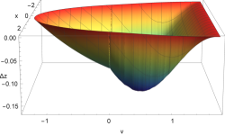
Figure 6: Solutions for the extremal volume, for $l=6$, $r_{h}=1$ and $t=1.75$. On the left we plot the solution; on the right we plot the difference $\Delta z$ between the solution and the pseudosolution.

The geodesics forming the boundary of the HRT surface are not smooth, this is expected from the solutions shown in Fig. 5. As can be seen, there are significant differences between the numerical solution and the pseudosolution.

3.5 Time dependence of volume

We are then interested in the volume functional (3.16) evaluated on the equation of motion, which we denote by $V$. We regularize UV divergences by subtracting the AdS volume (3.3). The volume of the solution as a function of the time $t$ is shown in Fig. 7; for comparison, also the volume of the pseudosolution is displayed. The solution has indeed as expected a bigger volume. Fig. 7 confirms that the volume of the pseudosolution is indeed a good approximation both for early $t\approx 0$ and late $t\approx l/2$ times. For intermediate times, the discrepancy tends to increase with $l$. As can be seen, the plot of the volume of the numerical solution seems to be smoother than the one of the pseudosolution. In particular, the variation of the slope of the solution is less pronounced than the one of the pseudosolution.

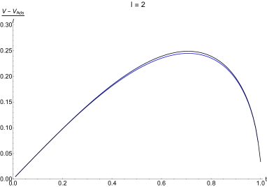
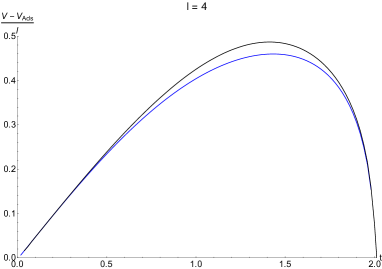
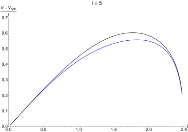
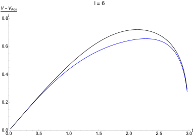
Figure 7: Time dependence of the volume $V$ of the solution (black), compared to the volume $\hat{V}$ of the pseudosolution (blue) for $l=2$ (up, left), $l=4$ (up, right), $l=5$ (left, bottom), $l=6$ (right, bottom). We set $r_{h}=1$.

3.6 Analytical results

Both at early times and at late times, the volume of the pseudosolution is a good approximation of the volume of the solution. It should be remarked that the pseudosolution in any case provides a lower bound of the volume of the solution.

When $l$ is large enough, typically larger than $1/r_{h}$, there are three stages in the evolution of the volume of the pseudosolution:

• Early times. If we replace the early time results eq. (B.1) in the volume expression eq. (3.14), we find, at the leading order in $l$:

  $$\frac{\hat{V}}{l}=\Lambda+r_{h}\,\tanh\frac{r_{h}t}{2}+\mathcal{O}(1/l)\,.$$ (3.20)

  This is true in both the regimes $r_{s}>r_{h}/\sqrt{2}$ and $r_{s}<r_{h}/\sqrt{2}$; the only assumption is that time is so early that eq. (B.1) can be trusted. From numerical evidence, it turns out that this part of the evolution continues for a time that scales as $\mathcal{O}(\log(r_{h}l))$.

  At early times, the pseudosolution is a good approximation to the full solution. In particular, one can safely trust the first order Taylor expansion of eq. (3.20), i.e.

  $$\frac{{V}}{l}=\Lambda+\frac{r_{h}^{2}t}{2}+\mathcal{O}(1/l)\,.$$ (3.21)

  This is further supported by the fact that $\tanh x\leq x$ and that the volume of the pseudosolution is a lower bound of the one of the solution. This agrees with the result in eq. (3.77) of [33] for the growth rate $\tilde{V}$ of the volume in a one-sided Vaidya black hole, which in our notation and for $d=2$ reads:

  $$\frac{d\tilde{V}}{dt}=\Omega_{k}\frac{r_{h}^{2}}{2}\,,$$ (3.22)

  where $\Omega_{k}$ is divergent and it corresponds to our boundary subregion size $l$ in the limit $l\rightarrow\infty$.

• Intermediate times, $\mathcal{O}(\log r_{h}l)<t<\frac{l}{2}-\frac{0.53}{r_{h}}$. An explicit analytical formula for the volume of the pseudosolution at large $l$ is derived in appendix C:

  $$\frac{\hat{V}}{l}\approx\Lambda+\frac{\mathcal{I}_{1}}{l}+(\Upsilon-1)\eta(r_{s})-\Upsilon\eta(r_{m})\,.$$ (3.23)

  where ${\mathcal{I}_{1}}$, $\Upsilon$, $\eta$ are defined in Appendix C. Unfortunately, at large $l$ we expect significant deviations between the solution and pseudosolution volumes. Nonetheless, this estimate is still useful because it provides a lower bound to the volume of the solution.

• Late times, $\frac{l}{2}-\frac{0.53}{r_{h}}<t<\frac{l}{2}$. We can approximate the volume of the pseudosolution as

  $$\frac{\hat{V}}{l}=\Lambda+\frac{r_{h}^{2}l}{4}\frac{\sqrt{r_{s}r_{h}(r_{h}-r_{s})(2r_{s}-r_{h})}}{(r_{s}-r_{h})^{2}+r_{s}^{2}}+\mathcal{O}(l^{0})\,,$$ (3.24)

  see appendix C for a derivation. The maximum of $\hat{V}$ is at $r_{s}=r_{h}/\sqrt{2}$ and scales as:

  $${\rm max}\,\left(\frac{\hat{V}}{l}\right)=\Lambda+\frac{lr_{h}^{2}}{8}\,.$$ (3.25)

  Using the approximation eq. (B.7), we find the following behaviour nearby $t\approx l/2$:

  $$r_{s}\approx r_{h}\left(1-\sqrt{\frac{r_{h}}{2}\left(\frac{l}{2}-t\right)}\right)\,,\qquad\frac{\hat{V}}{l}\approx\Lambda+l\left(\frac{r_{h}}{2}\right)^{9/4}\left(\frac{l}{2}-t\right)^{1/4}\,.$$ (3.26)

  Also in this regime we expect that this is a good approximation of the volume of the solution.

3.7 Discussion

The central charge of the boundary theory $c$, the final temperature $T$, entropy $S$ and complexity $\mathcal{C}_{V}$ can be expressed in terms of bulk quantities as follows

$$c=\frac{3}{2G}\,,\qquad T=\frac{r_{h}}{2\pi}\,,\qquad S=\frac{r_{h}l}{4G}\,,\qquad\mathcal{C}_{V}=\frac{V}{G}\,,$$ (3.27)

where we set the AdS radius $L_{AdS}=1$ by a choice of units. The regularized complexity, defined as $\Delta\mathcal{C}_{V}=\mathcal{C}_{V}-\mathcal{C}_{V}^{AdS}$, can be expressed as

$$\frac{\Delta\mathcal{C}_{V}}{l}=\frac{4\pi}{3}\,c\,T\,W_{\lambda}(\tau)\,,$$ (3.28)

where

$$\tau=2\pi T\,t\,,\qquad\lambda=2\pi T\,l\,,\qquad W_{\lambda}(\tau)=\frac{V_{\rm sol}-V_{\rm AdS}}{\lambda}\,.$$ (3.29)

The function $W_{\lambda}(\tau)$ is plotted in Fig. 8 for a few values of $\lambda$. For small $\tau$, from eq. (3.21) we find $W_{\lambda}\approx\tau/2$.

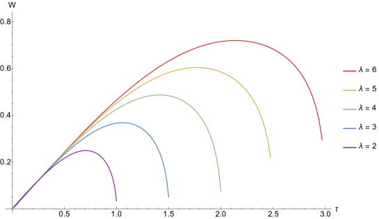
Figure 8: $W_{\lambda}$ as a function of $\tau$ for some values of $\lambda$.

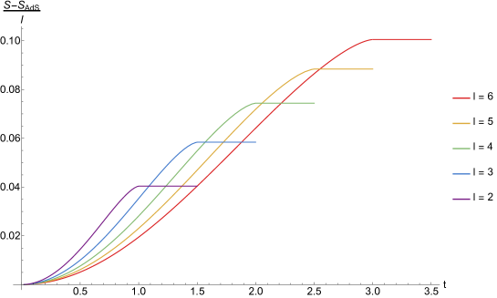
Figure 9: Entropy of the solution as a function of time for some values of $l$, with the diverging entropy of the vacuum AdS subtracted. Here we set $G=1$, $r_{h}=1$ for illustrative purposes.

It is interesting to compare the time behaviour of complexity with the one of entanglement entropy, which can be computed using eq. (109) of [30]. A plot is shown in Fig 9. While the behaviour of entanglement entropy interpolates between the value in AdS and the thermal one in a monotonic way during the quench, the behaviour of subregion complexity grows to a maximum which scales as $l^{2}$ and then goes back to the original value of empty AdS.

It is remarkable that, after thermalization, $\Delta\mathcal{C}_{V}=0$, eq. (3.4). From the geometrical point of view, this property follows from the Gauss-Bonnet theorem. From the point of view of the boundary field theory this behaviour looks rather counterintuitive. Indeed, for asymptotically AdS_d black branes, with $d>3$, this property does not hold [45]. On the other hand, in the small $l\,T$ regime, the calculations for $d>3$ in [54] should be correct. Then we expect that, also in this case, subregion complexity, after the initial growth stage, decreases at large times going back to a value which is much closer to the original one compared to its maximum.

We can qualitatively interpret this behaviour as follows. One of the most promising candidates for the field theory dual of subregion complexity is purification complexity, which is defined as the minimal pure state complexity among all possible purifications of the given mixed state [43]. At equilibrium, there is a maximal amount of possible pure microstates which corresponds to the given mixed macrostate. In this big community of states, it should not be surprising that the minimal complexity is small, due to the large number of samples. Instead, far away from equilibrium, the number of microstates which describe our density matrix is much smaller, and so we can expect that the minimal complexity is bigger.

We expect that the Lloyd’s bound [63] should apply only when subregion complexity coincides with the pure state one. This should be true only at early times, because the boundary effects are negligible. Indeed in this regime $W_{\lambda}\approx\tau/2$ and then we recover the result (3.22):

$$\frac{d{\mathcal{C}}}{dt}=8\pi M\,,\qquad M=\frac{l\,r_{h}^{2}}{16\pi G}\,,$$ (3.30)

where $M$ is the black hole mass. This is the same as the asymptotic complexity rate in time-independent black holes, and as such saturates the conjectured Lloyd’s bound. Moreover from figure 8 we see that, nearby $t=0$, the rate $\frac{d{\mathcal{C}}}{dt}$ is a decreasing function of time, and so the Lloyd bound is not violated also by subregion complexity at small time.

4 Conclusions

In this paper we studied the holographic subregion volume complexity for a line segment of length $l$ in the AdS₃ Vaidya geometry, in the limit of zero shell thickness eq. (2.5). We computed the extremal volume as a function of time numerically, and we found that both at early times $t\approx 0$ and at late times, nearby equilibrium $t\approx l/2$, the $x$-independent ansatz is a good approximation of the solution for the extremal volume. We give analytical expressions for the extremal volume in both the early and late time regimes, see eqs. (3.20) and (3.24,3.26). In particular, the maximum of the volume of the pseudosolution scales as $l^{2}$, see eq. (3.25). Since the pseudosolution is a lower bound of the solution, we expect that the maximum of the volume of the solution scales at least as $l^{2}$.

We were able to numerically study the full dependence of holographic subregion volume complexity (see figure 8) just for $r_{h}l\leq 6$. Figure 7 shows that the corrections from the $x$-independent pseudosolution become increasingly important as $l$ grows.

Several problems call for further investigation:

• It would be interesting to study larger values of $l$, because it is the regime where bigger deviations from the $x$-independent pseudosolution are expected. In particular, in [54, 57] it was conjectured that for large $l$ and intermediate times a linear increase regime of complexity holds, with a different slope compared to the early times regime. This conjecture was based on the calculation of the volume of the $x$-independent pseudosolution. However, since we showed that at large $l$ one should expect large deviation between the volumes of the solution and the pseudosolution, this conjecture should be revisited.

• Another open problem is to study the time evolution of subregion action complexity during a quench and to compare it to the volume. In many cases the action and the volume conjectures give qualitatively similar results (there are however some exceptions, see e.g. [60]), which makes hard to discriminate between them. Due to the large arbitrariness in several technical aspects of the definition of complexity in QFT, it could also be that each of the conjectures is dual to a different field theory definition of quantum computational complexity.

• It would be interesting to study complexity evolution during a quench in QFT. This was initiated in [61, 62] for free field theories.

• There are several possible definitions of subregion complexity in a quantum theory, for example purification and basis complexity [43]. It would be interesting to establish robust properties of these quantum information quantities, in order to eventually match them with holographic conjectures. Another interesting direction is fidelity [40].

Appendix

Appendix A Spacelike geodesics in the BTZ black hole

For completeness, in this appendix we briefly sketch the computation of spacelike geodesics in the BTZ black hole background, following [30]. Introducing the bulk time $t$, the metric is:

$$ds^{2}=-(r^{2}-r_{h}^{2})dt^{2}+\frac{dr^{2}}{r^{2}-r_{h}^{2}}+r^{2}dx^{2}\,.$$ (A.1)

The relation between $t$ and the Eddington-Finkelstein coordinate $v$ which is used in the main text is:

$$t=v-\frac{1}{2r_{h}}\log\frac{|r-r_{h}|}{r+r_{h}}\,.$$ (A.2)

Parameterizing the geodesic length by $\sigma$, the geodesic equations are:

$$-r_{h}E=-(r^{2}-r_{h}^{2})\dot{t}\,,\qquad r_{h}J=r^{2}\dot{x}\,,\qquad 1=-(r^{2}-r_{h}^{2})\dot{t}^{2}+\frac{\dot{r}^{2}}{r^{2}-r_{h}^{2}}+r^{2}\dot{x}^{2}\,,$$ (A.3)

where dot denotes derivative with respect to $\sigma$. The parameters $E$ and $J$ are respectively the constants of motion associated to $t$ and $x$ translation invariance, i.e. energy and angular momentum. The equations in (A.3) can be solved analytically (see [30]). The solutions are expressed as $x(r)$ and $v(r)$ in eqs. (2.12), (2.13). The boundary conditions are chosen in such a way that the solution is symmetric under $x\rightarrow-x$.

Appendix B Analytical approximations for the constraint equations

The constraints in eqs. (2.23) and (2.19) cannot be solved in closed form, and are also rather tricky to be solved numerically, due to the exponential accuracy which is needed at large $l$ and $t$. It is then useful to use some approximations which are valid respectively in the early and in the late time regime:

• Early time approximation

  At early time $r_{s}\rightarrow\infty$ and $r_{*}\approx 2/l$, so we can use the $r_{*}\ll r_{s}$ approximation in eqs. (2.23) and (2.19). This gives:

  $$r_{*}=\frac{2}{l}\,,\qquad r_{s}=\frac{r_{h}}{2}\coth\left(\frac{r_{h}t}{2}\right)\,,$$ (B.1)

  which provides a good description of the early evolution of the geodesic.

• Late time approximation

  If we formally set $t\rightarrow\infty$ in eq. (2.23), we find the solution:

  $$\hat{r}_{*}=r_{h}\frac{r_{s}(2r_{s}-r_{h})}{(r_{h}-r_{s})^{2}+r_{s}^{2}}\,.$$ (B.2)

  The curve (B.2) is shown in fig. 10, with several $l$-constant curves solving the constraint in eq. (2.19).

  

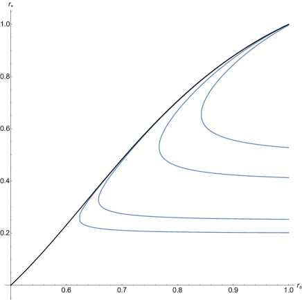
  Figure 10: Plot of the $t\rightarrow\infty$ limit curve $\hat{r}_{*}(r_{s})$ (black line), with $r_{h}=1$. The blue lines correspond to $l$-constant curves in the $(r_{s},r_{*})$ plane, see eq (2.19), for $l=4,5,8,10$ from top to bottom.

  The physical accessible region of parameters in the $(r_{s},r_{*})$ plane is below this curve; as a consequence, we have that $r_{s}>r_{h}/2$. In the late time regime we can parameterise the deviation from the curve (B.2) by

  $$r_{*}=\hat{r}_{*}-r_{h}\,\epsilon_{*}\,,$$ (B.3)

  with a small parameter $\epsilon_{*}\geq 0$. We can then solve eq. (2.19) at the leading order in $\epsilon_{*}$:

  $$\epsilon_{*}=\frac{8(1-\rho_{s})(2\rho_{s}-1)\rho_{s}^{3}}{(1-2\rho_{s}+2\rho_{s}^{2})^{2}}\frac{1}{\exp\left(r_{h}l-\frac{4(1-\rho_{s})}{2\rho_{s}-1}\right)-\frac{8\rho_{s}^{5}-20\rho_{s}^{4}+18\rho_{s}^{3}-7\rho_{s}+2}{\left(1-\rho_{s}\right)\left(2\rho_{s}^{2}-2\rho_{s}+1\right)}}\,,$$ (B.4)

  where we have introduced $\rho_{s}=r_{s}/r_{h}$. Taking the leading large $l$ term we find a simpler expression:

  $$\epsilon_{*}\approx\frac{8(1-\rho_{s})(2\rho_{s}-1)\rho_{s}^{3}}{(1-2\rho_{s}+2\rho_{s}^{2})^{2}}\exp\left(-r_{h}l+\frac{4(1-\rho_{s})}{2\rho_{s}-1}\right)\,,$$ (B.5)

  which is a good approximation when $\rho_{s}$ is not very nearby to $1/2$, which is true at large times.

  In order to find an approximate expression for $t$ as a function of $\rho_{s},\epsilon_{*}$, we use then the expansion (B.3) in the time constraint (2.23), which gives:

  $$r_{h}t=\frac{1}{2}\ln\left(\frac{8\left(1-\rho_{s}\right)\rho_{s}^{3}}{\epsilon_{*}\left(2\rho_{s}-1\right)\left(2\rho_{s}^{2}-2\rho_{s}+1\right){}^{2}}\right)\,.$$ (B.6)

  Inserting also the value of $\epsilon_{*}$ from eq. (B.5), we get

  $$r_{h}t=\frac{1}{2}\left(r_{h}l-\frac{4\left(1-\rho_{s}\right)}{2\rho_{s}-1}-\ln\left(\left(2\rho_{s}-1\right){}^{2}\right)\right)\,.$$ (B.7)

  Note that $\rho_{s}=1/\sqrt{2}$ corresponds to:

  $$r_{h}t=\frac{r_{h}l}{2}-\sqrt{2}-\ln\left(\sqrt{2}-1\right)\approx\frac{r_{h}l}{2}-0.53\,.$$ (B.8)

Appendix C The volume of the pseudosolution at late time

The approximation in this appendix refer to the limit $l,t\gg 1/r_{h}$ and to the regime in which $r_{*}\approx\hat{r}_{*}$. We will extensively use the results of appendix B. Let us write the volume of the pseudosolution eq. (3.14) as:

$$\hat{V}=\mathcal{I}_{1}+\mathcal{I}_{2}+\mathcal{I}_{3}+\mathcal{I}_{4}\,,$$ (C.1)

where

$$\mathcal{I}_{1}=-\pi+2\frac{\sqrt{r_{s}^{2}-r_{*}^{2}}}{r_{*}}+2\arcsin\frac{r_{*}}{r_{s}}\,,\qquad\mathcal{I}_{2}=l\int_{r_{s}}^{\Lambda}\psi(r)dr\,,$$ (C.2)

$$\mathcal{I}_{3}=\int_{r_{s}}^{\Lambda}\psi(r)\,\kappa(r)dr\,,\qquad\mathcal{I}_{4}=\theta\left(\frac{r_{h}}{\sqrt{2}}-r_{s}\right)l\,\Upsilon\int_{r_{m}}^{r_{s}}\psi(r)\,dr\,,$$ (C.3)

where

$$\kappa(r) = \frac{1}{r_{h}}\ln\frac{r^{2}-r_{*}\,r_{h}+\sqrt{r^{4}+\left[-1+\frac{r_{h}^{2}\left(r_{s}^{2}-r_{*}^{2}\right)}{4r_{s}^{4}}-\frac{r_{*}^{2}}{r_{h}^{2}}\right]r_{h}^{2}\,r^{2}+r_{*}^{2}\,r_{h}^{2}}}{r^{2}+r_{*}\,r_{h}+\sqrt{r^{4}+\left[-1+\frac{r_{h}^{2}\left(r_{s}^{2}-r_{*}^{2}\right)}{4r_{s}^{4}}-\frac{r_{*}^{2}}{r_{h}^{2}}\right]r_{h}^{2}\,r^{2}+r_{*}^{2}\,r_{h}^{2}}}\,,$$

$$\Upsilon = \left[\frac{1}{r_{h}l}\ln\frac{1-\frac{r_{h}^{2}\left(r_{s}^{2}-r_{*}^{2}\right)}{4r_{s}^{4}}+\frac{r_{*}^{2}}{r_{h}^{2}}-2\frac{r_{*}}{r_{h}}}{1-\frac{r_{h}^{2}\left(r_{s}^{2}-r_{*}^{2}\right)}{4r_{s}^{4}}+\frac{r_{*}^{2}}{r_{h}^{2}}+2\frac{r_{*}}{r_{h}}}+2\right]\,.$$ (C.4)

At late times we can use the following approximation, which can be derived from eq. (B.3):

$$r_{m}\approx\sqrt{\hat{r}_{*}r_{h}}+\sqrt{\epsilon_{*}}\sqrt{\frac{r_{h}^{3}(r_{h}^{2}-2r_{s}^{2})}{8r_{s}^{3}}}+\mathcal{O}(\epsilon_{*})\,,$$ (C.5)

where we have used the property $r_{s}>r_{h}/2$, which is always valid.

The calculation of the various term proceeds as follows:

• Let us focus on $\mathcal{I}_{4}$. Due to the Heaviside $\theta$, this term is non vanishing just in the intermediate time window eq. (B.8), i.e.

  $$t<\frac{l}{2}-\frac{0.53}{r_{h}}\,.$$ (C.6)

  Using the expansion in eq. (B.3), we can approximate

  $$\Upsilon=2+\frac{1}{r_{h}l}\ln\frac{\epsilon_{*}(r_{h}^{2}-2r_{s}^{2})r_{h}^{2}}{8\hat{r}_{*}r_{s}^{3}}+\mathcal{O}(\epsilon_{*})\approx 1+\frac{1}{r_{h}l}\left(\frac{4(1-\rho_{s})}{2\rho_{s}-1}+\ln\frac{(1-\rho_{s})(1-2\rho_{s}^{2})}{\rho_{s}(1-2\rho_{s}+2\rho_{s}^{2})}\right)\,,$$ (C.7)

  where we have used the late time approximation in eq. (B.5). We can also use the approximation:

  $$\psi(r)=r\,\frac{\sqrt{r^{2}-\hat{r}_{*}^{2}}}{\sqrt{(r^{2}-\hat{r}_{*}r_{h})^{2}+\mathcal{O}(\epsilon_{*})}}\,.$$ (C.8)

  This gives:

  $$\mathcal{I}_{4}\approx\theta\left(\frac{r_{h}}{\sqrt{2}}-r_{s}\right)l\,\Upsilon\int_{r_{m}}^{r_{s}}dr\,r\,\frac{\sqrt{r^{2}-\hat{r}_{*}^{2}}}{r^{2}-\hat{r}_{*}r_{h}}\,.$$ (C.9)

  This integral has a cutoff at $r_{m}\approx\sqrt{r_{h}\hat{r}_{*}}+\mathcal{O}(\sqrt{\epsilon_{*}})$, and so it is a good approximation to drop the order $\epsilon_{*}$ term in the denominator. This can now be evaluated analytically, using:

  $$\eta(r)=\int dr\,r\frac{\sqrt{r^{2}-\hat{r}_{*}^{2}}}{(r^{2}-\hat{r}^{*}r_{h})}=\sqrt{r^{2}-\hat{r}_{*}^{2}}+\frac{1}{2}\sqrt{(r_{h}-\hat{r}_{*})\hat{r}_{*}}\ln\left|\frac{\sqrt{(r_{h}-\hat{r}_{*})\hat{r}_{*}}-\sqrt{r^{2}-\hat{r}_{*}^{2}}}{\sqrt{(r_{h}-\hat{r}_{*})\hat{r}_{*}}+\sqrt{r^{2}-\hat{r}_{*}^{2}}}\right|\,.$$ (C.10)

  We finally get:

  $$\mathcal{I}_{4}\approx\theta\left(\frac{r_{h}}{\sqrt{2}}-r_{s}\right)l\,\Upsilon\left(\eta(r_{s})-\eta(r_{m})\right)\,.$$ (C.11)

• Let us consider $\mathcal{I}_{2}$, which at large time can be approximated as:

  $$\mathcal{I}_{2}\approx l\int_{r_{s}}^{\Lambda}dr\,r\sqrt{\frac{r^{2}-\hat{r}_{*}^{2}}{(r^{2}-\hat{r}_{*}r_{h})^{2}+\epsilon_{*}A(r)}}\,,\,\qquad A(r)=\frac{\hat{r}_{*}\left(r^{2}\left(4r_{s}^{4}r_{h}^{2}+r_{h}^{6}\right)-4r_{s}^{4}r_{h}^{4}\right)}{2r_{h}r_{s}^{4}}\,.$$ (C.12)

  It is useful to use the following properties:

  $$\begin{cases}{\rm for}\,\,\,r_{s}=\frac{r_{h}}{\sqrt{2}}\,\,\,{\rm and}\,\,\,r_{s}=r_{h}\,,\qquad&r_{s}=\sqrt{\hat{r}_{*}r_{h}}\\ {\rm for}\,\,\,r_{s}<\frac{r_{h}}{\sqrt{2}}\,,\qquad&r_{s}>\sqrt{\hat{r}_{*}r_{h}}\\ {\rm for}\,\,\,r_{h}>r_{s}>\frac{r_{h}}{\sqrt{2}}\,,\qquad&r_{s}<\sqrt{\hat{r}_{*}r_{h}}\end{cases}$$ (C.13)

  For this reason, we should separate two cases:

  • For $r_{s}<\frac{r_{h}}{\sqrt{2}}$ we have that $r_{s}>\sqrt{\hat{r}_{*}r_{h}}$ and so the $\epsilon_{*}$ term at the denominator is negligible:

    $$\mathcal{I}_{2}\approx\theta\left(\frac{r_{h}}{\sqrt{2}}-r_{s}\right)l\,(\Lambda-\eta(r_{s}))\,.$$ (C.14)

  • For $r_{s}>\frac{r_{h}}{\sqrt{2}}$ it is convenient to split

    $$\mathcal{I}_{2} = \mathcal{I}_{2}^{a}+\mathcal{I}_{2}^{b}\,,\qquad\mathcal{I}_{2}^{a}=l\int_{r_{s}}^{\sqrt{\hat{r}_{*}r_{h}}}dr\,r\frac{\sqrt{r^{2}-\hat{r}_{*}^{2}}}{\sqrt{(r^{2}-\hat{r}_{*}r_{h})^{2}+\epsilon_{*}A}}\,,$$

    $$\mathcal{I}_{2}^{b} = l\int_{\sqrt{\hat{r}_{*}r_{h}}}^{\Lambda}dr\,r\frac{\sqrt{r^{2}-\hat{r}_{*}^{2}}}{\sqrt{(r^{2}-\hat{r}_{*}r_{h})^{2}+\epsilon_{*}A(r)}}$$ (C.15)

    We will not need to evaluate $\mathcal{I}_{2}^{a}$, because we will show that it is cancelled by a term in $\mathcal{I}_{3}$. We can approximate $\mathcal{I}_{2}^{b}$ by noting that the term proportional to $\epsilon_{*}$ at the denominator acts as an effective cutoff of the integral:

    $$\mathcal{I}_{2}^{b}\approx l\int_{\tilde{r}}^{\Lambda}dr\,r\frac{\sqrt{r^{2}-\hat{r}_{*}^{2}}}{(r^{2}-\hat{r}_{*}r_{h})}\,,\qquad\tilde{r}=\sqrt{r_{*}r_{h}+\sqrt{\epsilon_{*}A(\sqrt{\hat{r}_{*}r_{h}})}}\,.$$ (C.16)

    Using eqs. (C.10) and (B.4) we find the leading $l$ behaviour:

    $$\mathcal{I}_{2}^{b}\approx l\Lambda+\frac{\sqrt{r_{s}r_{h}\left(-2r_{s}^{2}+3r_{s}r_{h}-r_{h}^{2}\right)}}{4\left(2r_{s}^{2}-2r_{s}r_{h}+r_{h}^{2}\right)}r_{h}^{2}l^{2}+\mathcal{O}(l)\,.$$ (C.17)

• We now approximate $\mathcal{I}_{3}$. In the limit $r_{*}\rightarrow\hat{r}_{*}$, we find that:

  $$\kappa(r)=\frac{1}{r_{h}}\ln\left(\frac{2\rho^{2}\rho_{s}^{2}-2\rho^{2}\rho_{s}+\rho^{2}-2\rho_{s}^{2}+\rho_{s}+\left|\rho^{2}\left(2\rho_{s}^{2}-2\rho_{s}+1\right)-2\rho_{s}^{2}+\rho_{s}\right|}{2\rho^{2}\rho_{s}^{2}-2\rho^{2}\rho_{s}+\rho^{2}+2\rho_{s}^{2}-\rho_{s}+\left|(\rho^{2}\left(2\rho_{s}^{2}-2\rho_{s}+1\right)-2\rho_{s}^{2}+\rho_{s}\right|}\right)\,,$$ (C.18)

  where we introduced $\rho=r/r_{h}$. It is useful to consider separately the following two cases:

  • If $r_{s}<r_{h}/\sqrt{2}$, then

    $$\rho^{2}\left(2\rho_{s}^{2}-2\rho_{s}+1\right)-2\rho_{s}^{2}+\rho_{s}>0$$ (C.19)

    for every $r_{s}<r<\Lambda$ and the factor in the integrand is finite and suppressed in the large $l$ limit.

  • If $r_{s}>r_{h}/\sqrt{2}$, then eq. (C.19) is valid just for $r>\sqrt{r_{*}r_{h}}$, and again gives a negligible contribution. For $r<\sqrt{r_{*}r_{h}}$ we have to change a sign and we get that the factor in the integrand is:

    $$\kappa(r)=\frac{1}{r_{h}}\ln\left(-\frac{\epsilon_{*}\left(\rho^{2}\left(4\rho_{s}^{5}-2\rho_{s}^{3}+2\rho_{s}-1\right)+2\left(1-2\rho_{s}\right)\rho_{s}^{4}\right)}{4\rho_{s}^{4}\left(2\rho_{s}-1\right)\left(\rho^{2}\left(2\rho_{s}^{2}-2\rho_{s}+1\right)-2\rho_{s}^{2}+\rho_{s}\right)}\right)\,.$$ (C.20)

    Inserting $\epsilon_{*}$ from the solution in eq. (B.5), we find that the log factor in the integrand simplifies to $-l+\mathcal{O}(l^{0})$, which cancels $\mathcal{I}_{2}^{a}$.

Adding up all the contributions, we find eq. (3.23) for $r_{s}<r_{h}/\sqrt{2}$ and eq. (3.24) for $r_{s}>r_{h}/\sqrt{2}$.

References

- [1] S. Ryu and T. Takayanagi, Phys. Rev. Lett. 96 (2006) 181602 doi:10.1103/PhysRevLett.96.181602 [hep-th/0603001].
- [2] H. Casini, M. Huerta and R. C. Myers, JHEP 1105 (2011) 036 doi:10.1007/JHEP05(2011)036 [arXiv:1102.0440 [hep-th]].
- [3] A. Lewkowycz and J. Maldacena, JHEP 1308 (2013) 090 doi:10.1007/JHEP08(2013)090 [arXiv:1304.4926 [hep-th]].
- [4] J. D. Bekenstein, Phys. Rev. D 7 (1973) 2333. doi:10.1103/PhysRevD.7.2333
- [5] L. Susskind, [Fortsch. Phys. 64 (2016) 24] Addendum: Fortsch. Phys. 64 (2016) 44 doi:10.1002/prop.201500093, 10.1002/prop.201500092 [arXiv:1403.5695 [hep-th], arXiv:1402.5674 [hep-th]].
- [6] D. Stanford and L. Susskind, Phys. Rev. D 90 (2014) no.12, 126007 doi:10.1103/PhysRevD.90.126007 [arXiv:1406.2678 [hep-th]].
- [7] L. Susskind, Fortsch. Phys. 64 (2016) 49 doi:10.1002/prop.201500095 [arXiv:1411.0690 [hep-th]].
- [8] Michael A. Nielsen, Quantum Information & Computation, Volume 6 Issue 3, May 2006, Pages 213-262, [arXiv:quant-ph/0502070]
- [9] Mark R. Dowling, Michael A. Nielsen, Quantum Information & Computation, Volume 8 Issue 10, November 2008, Pages 861-899, [arXiv:quant-ph/0701004]
- [10] R. Jefferson and R. C. Myers, JHEP 1710 (2017) 107 doi:10.1007/JHEP10(2017)107 [arXiv:1707.08570 [hep-th]].
- [11] S. Chapman, M. P. Heller, H. Marrochio and F. Pastawski, Phys. Rev. Lett. 120 (2018) no.12, 121602 doi:10.1103/PhysRevLett.120.121602 [arXiv:1707.08582 [hep-th]].
- [12] K. Hashimoto, N. Iizuka and S. Sugishita, Phys. Rev. D 96 (2017) no.12, 126001 doi:10.1103/PhysRevD.96.126001 [arXiv:1707.03840 [hep-th]].
- [13] P. Caputa, N. Kundu, M. Miyaji, T. Takayanagi and K. Watanabe, JHEP 1711 (2017) 097 doi:10.1007/JHEP11(2017)097 [arXiv:1706.07056 [hep-th]].
- [14] A. Bhattacharyya, P. Caputa, S. R. Das, N. Kundu, M. Miyaji and T. Takayanagi, arXiv:1804.01999 [hep-th].
- [15] S. Chapman, J. Eisert, L. Hackl, M. P. Heller, R. Jefferson, H. Marrochio and R. C. Myers, SciPost Phys. 6 (2019) no.3, 034 doi:10.21468/SciPostPhys.6.3.034 [arXiv:1810.05151 [hep-th]].
- [16] A. R. Brown, D. A. Roberts, L. Susskind, B. Swingle and Y. Zhao, Phys. Rev. Lett. 116 (2016) no.19, 191301 doi:10.1103/PhysRevLett.116.191301 [arXiv:1509.07876 [hep-th]].
- [17] A. R. Brown, D. A. Roberts, L. Susskind, B. Swingle and Y. Zhao, Phys. Rev. D 93 (2016) no.8, 086006 doi:10.1103/PhysRevD.93.086006 [arXiv:1512.04993 [hep-th]].
- [18] L. Lehner, R. C. Myers, E. Poisson and R. D. Sorkin, Phys. Rev. D 94 (2016) no.8, 084046 doi:10.1103/PhysRevD.94.084046 [arXiv:1609.00207 [hep-th]].
- [19] R. G. Cai, S. M. Ruan, S. J. Wang, R. Q. Yang and R. H. Peng, JHEP 1609 (2016) 161 doi:10.1007/JHEP09(2016)161 [arXiv:1606.08307 [gr-qc]].
- [20] S. Chapman, H. Marrochio and R. C. Myers, JHEP 1701 (2017) 062 doi:10.1007/JHEP01(2017)062 [arXiv:1610.08063 [hep-th]].
- [21] D. Carmi, S. Chapman, H. Marrochio, R. C. Myers and S. Sugishita, JHEP 1711 (2017) 188 doi:10.1007/JHEP11(2017)188 [arXiv:1709.10184 [hep-th]].
- [22] M. Alishahiha, A. Faraji Astaneh, A. Naseh and M. H. Vahidinia, JHEP 1705 (2017) 009 doi:10.1007/JHEP05(2017)009 [arXiv:1702.06796 [hep-th]].
- [23] M. Ghodrati, Phys. Rev. D 96 (2017) no.10, 106020 doi:10.1103/PhysRevD.96.106020 [arXiv:1708.07981 [hep-th]].
- [24] R. Auzzi, S. Baiguera and G. Nardelli, JHEP 1806 (2018) 063 doi:10.1007/JHEP06(2018)063 [arXiv:1804.07521 [hep-th]].
- [25] R. Auzzi, S. Baiguera, M. Grassi, G. Nardelli and N. Zenoni, JHEP 1809 (2018) 013 doi:10.1007/JHEP09(2018)013 [arXiv:1806.06216 [hep-th]].
- [26] H. Dimov, R. C. Rashkov and T. Vetsov, Phys. Rev. D 99 (2019) no.12, 126007 doi:10.1103/PhysRevD.99.126007 [arXiv:1902.02433 [hep-th]].
- [27] M. Alishahiha, A. Faraji Astaneh, M. R. Mohammadi Mozaffar and A. Mollabashi, JHEP 1807 (2018) 042 doi:10.1007/JHEP07(2018)042 [arXiv:1802.06740 [hep-th]].
- [28] M. Flory and N. Miekley, JHEP 1905 (2019) 003 doi:10.1007/JHEP05(2019)003 [arXiv:1806.08376 [hep-th]].
- [29] M. Flory, JHEP 1905 (2019) 086 doi:10.1007/JHEP05(2019)086 [arXiv:1902.06499 [hep-th]].
- [30] V. Balasubramanian et al., Phys. Rev. D 84 (2011) 026010 doi:10.1103/PhysRevD.84.026010 [arXiv:1103.2683 [hep-th]].
- [31] M. Moosa, JHEP 1803 (2018) 031 doi:10.1007/JHEP03(2018)031 [arXiv:1711.02668 [hep-th]].
- [32] M. Moosa, Phys. Rev. D 97 (2018) no.10, 106016 doi:10.1103/PhysRevD.97.106016 [arXiv:1712.07137 [hep-th]].
- [33] S. Chapman, H. Marrochio and R. C. Myers, JHEP 1806 (2018) 046 doi:10.1007/JHEP06(2018)046 [arXiv:1804.07410 [hep-th]].
- [34] S. Chapman, H. Marrochio and R. C. Myers, JHEP 1806 (2018) 114 doi:10.1007/JHEP06(2018)114 [arXiv:1805.07262 [hep-th]].
- [35] M. Nozaki, T. Numasawa and T. Takayanagi, JHEP 1305 (2013) 080 doi:10.1007/JHEP05(2013)080 [arXiv:1302.5703 [hep-th]].
- [36] D. S. Ageev, I. Y. Aref’eva, A. A. Bagrov and M. I. Katsnelson, JHEP 1808 (2018) 071 doi:10.1007/JHEP08(2018)071 [arXiv:1803.11162 [hep-th]].
- [37] D. S. Ageev, arXiv:1902.03632 [hep-th].
- [38] B. Czech, J. L. Karczmarek, F. Nogueira and M. Van Raamsdonk, Class. Quant. Grav. 29 (2012) 155009 doi:10.1088/0264-9381/29/15/155009 [arXiv:1204.1330 [hep-th]].
- [39] V. E. Hubeny and M. Rangamani, JHEP 1206 (2012) 114 doi:10.1007/JHEP06(2012)114 [arXiv:1204.1698 [hep-th]].
- [40] M. Alishahiha, Phys. Rev. D 92 (2015) no.12, 126009 doi:10.1103/PhysRevD.92.126009 [arXiv:1509.06614 [hep-th]].
- [41] D. Carmi, R. C. Myers and P. Rath, JHEP 1703 (2017) 118 doi:10.1007/JHEP03(2017)118 [arXiv:1612.00433 [hep-th]].
- [42] V. E. Hubeny, M. Rangamani and T. Takayanagi, JHEP 0707 (2007) 062 doi:10.1088/1126-6708/2007/07/062 [arXiv:0705.0016 [hep-th]].
- [43] C. A. Agón, M. Headrick and B. Swingle, JHEP 1902 (2019) 145 doi:10.1007/JHEP02(2019)145 [arXiv:1804.01561 [hep-th]].
- [44] E. Cáceres, J. Couch, S. Eccles and W. Fischler, arXiv:1811.10650 [hep-th].
- [45] O. Ben-Ami and D. Carmi, JHEP 1611 (2016) 129 doi:10.1007/JHEP11(2016)129 [arXiv:1609.02514 [hep-th]].
- [46] R. Abt, J. Erdmenger, H. Hinrichsen, C. M. Melby-Thompson, R. Meyer, C. Northe and I. A. Reyes, Fortsch. Phys. 66 (2018) no.6, 1800034 doi:10.1002/prop.201800034 [arXiv:1710.01327 [hep-th]].
- [47] R. Abt, J. Erdmenger, M. Gerbershagen, C. M. Melby-Thompson and C. Northe, JHEP 1901 (2019) 012 doi:10.1007/JHEP01(2019)012 [arXiv:1805.10298 [hep-th]].
- [48] M. Alishahiha, K. Babaei Velni and M. R. Mohammadi Mozaffar, arXiv:1809.06031 [hep-th].
- [49] P. Roy and T. Sarkar, Phys. Rev. D 96 (2017) no.2, 026022 doi:10.1103/PhysRevD.96.026022 [arXiv:1701.05489 [hep-th]].
- [50] P. Roy and T. Sarkar, Phys. Rev. D 97 (2018) no.8, 086018 doi:10.1103/PhysRevD.97.086018 [arXiv:1708.05313 [hep-th]].
- [51] E. Bakhshaei, A. Mollabashi and A. Shirzad, Eur. Phys. J. C 77 (2017) no.10, 665 doi:10.1140/epjc/s10052-017-5247-1 [arXiv:1703.03469 [hep-th]].
- [52] A. Bhattacharya, K. T. Grosvenor and S. Roy, arXiv:1905.02220 [hep-th].
- [53] R. Auzzi, S. Baiguera, A. Mitra, G. Nardelli and N. Zenoni, arXiv:1906.09345 [hep-th].
- [54] B. Chen, W. M. Li, R. Q. Yang, C. Y. Zhang and S. J. Zhang, JHEP 1807 (2018) 034 doi:10.1007/JHEP07(2018)034 [arXiv:1803.06680 [hep-th]].
- [55] Y. Ling, Y. Liu and C. Y. Zhang, Eur. Phys. J. C 79 (2019) no.3, 194 doi:10.1140/epjc/s10052-019-6696-5 [arXiv:1808.10169 [hep-th]].
- [56] Y. T. Zhou, M. Ghodrati, X. M. Kuang and J. P. Wu, arXiv:1907.08453 [hep-th].
- [57] Y. Ling, Y. Liu, C. Niu, Y. Xiao and C. Y. Zhang, arXiv:1908.06432 [hep-th].
- [58] M. Banados, C. Teitelboim and J. Zanelli, Phys. Rev. Lett. 69 (1992) 1849 doi:10.1103/PhysRevLett.69.1849 [hep-th/9204099].
- [59] M. Banados, M. Henneaux, C. Teitelboim and J. Zanelli, Phys. Rev. D 48 (1993) 1506 Erratum: [Phys. Rev. D 88 (2013) 069902] doi:10.1103/PhysRevD.48.1506, 10.1103/PhysRevD.88.069902 [gr-qc/9302012].
- [60] S. Chapman, D. Ge and G. Policastro, JHEP 1905 (2019) 049 doi:10.1007/JHEP05(2019)049 [arXiv:1811.12549 [hep-th]].
- [61] D. W. F. Alves and G. Camilo, JHEP 1806 (2018) 029 doi:10.1007/JHEP06(2018)029 [arXiv:1804.00107 [hep-th]].
- [62] H. A. Camargo, P. Caputa, D. Das, M. P. Heller and R. Jefferson, Phys. Rev. Lett. 122 (2019) no.8, 081601 doi:10.1103/PhysRevLett.122.081601 [arXiv:1807.07075 [hep-th]].
- [63] S. Lloyd, Nature 406 (2000), no. 6799 1047-1054.