An Empirical Comparison on Imitation Learning and Reinforcement Learning for Paraphrase Generation

Abstract

Generating paraphrases from given sentences involves decoding words step by step from a large vocabulary. To learn a decoder, supervised learning which maximizes the likelihood of tokens always suffers from the exposure bias. Although both reinforcement learning (RL) and imitation learning (IL) have been widely used to alleviate the bias, the lack of direct comparison leads to only a partial image on their benefits. In this work, we present an empirical study on how RL and IL can help boost the performance of generating paraphrases, with the pointer-generator as a base model . Experiments on the benchmark datasets show that (1) imitation learning is constantly better than reinforcement learning; and (2) the pointer-generator models with imitation learning outperform the state-of-the-art methods with a large margin.

1 Introduction

Generating paraphrases is a fundamental research problem that could benefit many other NLP tasks, such as machine translation (Bahdanau et al., 2014), text generation (Radford et al., 2019), document summarization (Chopra et al., 2016), and question answering (McCann et al., 2018). Although various methods have been developed (Zhao et al., 2009; Quirk et al., 2004; Barzilay and Lee, 2003), the recent progress on paraphrase generation is mainly from neural network modeling (Prakash et al., 2016). Particularly, the encoder-decoder framework is widely adopted (Cho et al., 2015), where the encoder takes source sentences as inputs and the decoder generates the corresponding paraphrase for each input sentence.

In supervised learning, a well-known challenge of generating paraphrases is the exposure bias: the current prediction is conditioned on the ground truth during training but on previous predictions during decoding, which may accumulate and propagate the error when generating the text. To address this challenge, prior work (Li et al., 2018) suggests to utilize the exploration strategy in reinforcement learning (RL). However, training with the RL algorithms is not trivial and often hardly works in practice (Dayan and Niv, 2008). A typical way of using RL in practice is to train the model with supervised learning (Ranzato et al., 2015; Shen et al., 2015; Bahdanau et al., 2016), which leverages the supervision information from training data and alleviate the exposure bias to some extent. In the middle ground between RL and supervised learning, a well-known category is imitation learning (IL) (Daumé et al., 2009; Ross et al., 2011), which has been used in structured prediction (Bagnell et al., 2007) and other sequential prediction tasks (Bengio et al., 2015).

In this work, we conduct an empirical comparison between RL and IL to demonstrate the pros and cons of using them for paraphrase generation. We first propose a unified framework to include some popular learning algorithms as special cases, such as the Reinforce algorithm (Williams, 1992) in RL and the Dagger algorithm (Ross et al., 2011) in IL. To better understand the value of different learning techniques, we further offer several variant learning algorithms based on the RL framework. Experiments on the benchmark datasets show: (1) the Dagger algorithm is better than the Reinforce algorithm and its variants on paraphrase generation, (2) the Dagger algorithm with a certain setting gives the best results, which outperform the previous state-of-the-art with about 13% on the average evaluation score. We expect this work will shed light on how to choose between RL and IL, and alleviate the exposure bias for other text generation tasks.

2 Method

Given an input sentence $\bm{x}=(x_{1},x_{2},\cdots,x_{S})$ with length $S$, a paraphrase generation model outputs a new sentence $\bm{y}=(y_{1},y_{2},\cdots,y_{T})$ with length $T$ that shares the same meaning with $\bm{x}$. The widely adopted framework on paraphrase generation is the encoder-decoder framework (Cho et al., 2014). The encoder reads sentence $\bm{x}$ and represents it as a single numeric vector or a set of numeric vectors. The decoder defines a probability function $p(y_{t}\mid\bm{y}_{\leq t-1},\bm{x};\bm{\theta})$, where $\bm{y}_{\leq t-1}=(y_{1},y_{2},\dots,y_{t-1})$ and $\bm{\theta}$ is the collection of model parameters,

$$p(y_{t}\mid\bm{y}_{\leq t-1},\bm{x};\bm{\theta})=\text{softmax}\left(\mathbf{W}\bm{h}_{t}\right)$$ (1)

with $\bm{h}_{t}=\bm{f}(\bm{h}_{t-1},y_{t-1},\bm{x})$, where $\bm{f}$ as a nonlinear transition function and $\mathbf{W}\in\bm{\theta}$ as a parameter matrix. We use the pointer-generator model (See et al., 2017) as the base model, which is state-of-the-art model on paragraph generation (Li et al., 2018). We skip the detail explanation of this model and please refer to (See et al., 2017) for further information.

2.1 Basic Learning Algorithms

To facilitate the comparison between RL and IL, we propose a unified framework with the following objective function. Given a training example $(\bm{x},\bm{y})$, the objective function is defined as

$$L(\bm{\theta})=\big{\{}\sum_{t=1}^{T}\log\pi_{\theta}(\tilde{y}_{t}\mid\bm{h}_{t})\big{\}}\cdot r(\tilde{\bm{y}},\bm{y}),$$ (2)

Following the terminology in RL and IL, we rename $P(\tilde{y}_{t}\mid\bm{y}_{\leq t-1},\bm{x};\bm{\theta})$ as the the policy function $\pi_{\theta}(\tilde{y}_{t}\mid\bm{h}_{t})$. That implies taking an action based on the current observation, where the action is picking a word $\tilde{y}_{t}$ from the vocabulary $\mathcal{V}$. $r(\tilde{\bm{y}},\bm{y})$ is a reward function with $r(\tilde{\bm{y}},\bm{y})=1$ if $\tilde{\bm{y}}=\bm{y}$. In our experiments, We use the ROUGE-2 score (Lin, 2004) as the reward function. Algorithm 1 presents how to optimize $L(\bm{\theta})$ in the online learning fashion. As shown in the pseudocode, the schedule rates $(\alpha,\beta)$ and the decoding function $\texttt{Decode}(\cdot)$ are the keys to understand the special cases of this unified framework.

Algorithm 1 Online learning

1:  Input: A training example $(\bm{x}^{(i)},\bm{y}^{(i)})$, current schedule rates $\alpha^{(i)},\beta^{(i)}\in[0,1]$, learning rate $\eta$

2:  Initialize $L(\bm{\theta})\leftarrow 0$

3:  for $t=1,\dots,T$ do

4:     $p_{1},p_{2}\sim\text{Uniform}(0,1)$

5:     $\tilde{y}_{t-1}\leftarrow y_{t-1}~{}\textbf{if}~{}(p_{1}<\alpha^{(i)})~{}\textbf{else}~{}\hat{y}_{t-1}$

6:     $\bm{h}_{t}=\bm{f}(\bm{h}_{t-1},\tilde{y}_{t-1},\bm{x})$

7:     $\hat{y}_{t}\leftarrow\texttt{Decode}(\pi(y\mid\bm{h}_{t}))$

8:     $\tilde{y}_{t}\leftarrow y_{t}~{}\textbf{if}~{}(p_{2}<\beta^{(i)})~{}\textbf{else}~{}\hat{y}_{t}$

9:     $L(\bm{\theta})\leftarrow L(\bm{\theta})+\log\pi(\tilde{y}_{t}\mid\bm{h}_{t})$

10:  end for

11:  $\delta\bm{\theta}\leftarrow\nabla_{\bm{\theta}}L(\bm{\theta})\cdot r(\tilde{\bm{y}^{(i)}},\bm{y}^{(i)})$

12:  $\bm{\theta}\leftarrow\bm{\theta}+\eta\cdot\delta\bm{\theta}$

The Reinforce Algorithm.

When $\alpha=0$, $\beta=0$, and $\texttt{Decode}(\pi(y\mid\bm{h}_{t}))$ is defined as as:

$$\begin{split}&\texttt{Decode}(\pi_{\theta}(y\mid\bm{h}_{t-1}))\\ &~{}~{}~{}=\text{Random\_Sampling}(\pi_{\theta}(y\mid\bm{h}_{t-1})),\end{split}$$ (3)

Specifically, when $\alpha=\beta=0$, both $\tilde{y}_{t-1}$ and $\tilde{y}_{t}$ will choose the sampled values from the Decode function with policy $\pi_{\theta}$. It essentially samples a trajectory from the decoder $(\hat{y}_{1},\hat{y}_{2},\dots,\hat{y}_{T})$ as in the Reinforce algorithm. The reward is $r(\tilde{\bm{y}},\bm{y})=r(\hat{\bm{y}},\bm{y})$ once it has the entire trajectory $\hat{\bm{y}}$.

The Dagger Algorithm.

When $0<\alpha<1$, $\beta=1$, and $\texttt{Decode}(\pi(y\mid\bm{h}_{t}))$ is defined as as:

$$\texttt{Decode}(\pi_{\theta}(y\mid\bm{h}_{t-1}))=\operatorname*{argmax}_{y^{\prime}}\pi_{\theta}(y^{\prime}\mid\bm{h}_{t-1}).$$ (4)

Depending the value of $\alpha$, $\tilde{y}_{t-1}$ will choose between the ground truth $y_{t-1}$ and decoded value $\hat{y}_{t-1}$ with the function defined in Equation 4. On the other hand, $\tilde{y}_{t}$ will always choose the ground truth $y_{t}$ as $\beta=1$. Since $\tilde{\bm{y}}=\bm{y}$, we have $r(\tilde{\bm{y}},\bm{y})=1$ and the reward can be ignored from Equation 2. In imitation learning, ground truth sequence $\bm{y}$ is called expert actions. The Dagger algorithm (Ross et al., 2011) is also called scheduled sampling (Bengio et al., 2015) in recent deep learning literature. To be accurate, in the Dagger and the scheduled sampling, the $\alpha$ is dynamically changed during training. Typically, it starts from 1 and gradually decays to a certain value along with iterations. As shown in our experiments, the selection of decay scheme has a big impact on model performance.

The MLE Algorithm.

Besides, there is a trivial case when $\alpha=1,\beta=1$. In this case, $\tilde{y}_{t-1}$ and $\tilde{y}_{t}$ are equal to $y_{t-1}$ and $y_{t}$ respectively, and $r(\tilde{\bm{y}},\bm{y})=1$. Optimizing the objective function in Equation 2 is reduced to the maximum likelihood estimation (MLE).

2.2 Other Variant Algorithms

Inspired by the previous three special cases, we offer other algorithm variants with different combinations of $(\alpha,\beta)$, while the decoding function $\texttt{Decode}(\pi(y\mid\bm{h}_{t}))$ in the same as Equation 3 in all following variants.

• Reinforce-GTI (Reinforce with Ground Truth Input): $\alpha=1$, $\beta=0$. Unlike the Reinforce algorithm, Reinforce-GTI restricts the input to the decoder can only be ground truth words, which means $\tilde{y}_{t-1}=y_{t-1}$. This is a popular implementation in the deep reinforcement learning for Seq2Seq models (Keneshloo et al., 2018).

• Reinforce-SO (Reinforce with Sampled Output): $\alpha=1$, $0<\beta<1$. In terms of choosing the value of $\tilde{y}_{t}$ as output from the decoder, Reinforce-SO allows $\tilde{y}_{t}$ to select the ground truth $y_{t}$ with probability $\beta$.

• Reinforce-SIO (Reinforce with Sampled Input and Output): $0<\alpha<1$, $0<\beta<1$. Instead of always taking the ground truth $y_{t-1}$ as input, Reinforce-SIO further relaxes the constraint in Reinforce-SO and allows $\tilde{y}_{t-1}$ to be the decoded value $\hat{y}_{t-1}$ with probability $\alpha$.

Unless specified explicitly, an additional requirement when $0<\alpha,\beta<1$ is that its value decays to a certain value during training, which by default is 0.

3 Experiments

Dataset and Evaluation Metrics.

We evaluate our models on the Quora Question Pair Dataset , and the Twitter URL Paraphrasing Dataset (Lan et al., 2017) . Both datasets contain positive and negative examples of paraphrases, and we only keep the positive examples for our experiments as in prior work of paraphrase generation (Li et al., 2018; Patro et al., 2018). For the Quora dataset, we follows the configuration of (Li et al., 2018) and split the data into 100K training pairs, 30K testing pairs and 3K validation pairs. For the Twitter dataset, since our model cannot deal with the negative examples as (Li et al., 2018) do, we just obtain the 1-year 2,869,657 candidate pairs from https://languagenet.github.io, and filter out all negative examples. Finally, we divided the remaining dataset into 110K training pairs, 3K testing pairs and 1K validation pairs.

We use the following evaluation metrics to compare our models with other state-of-art neural networks: Rouge-1 and Rouge-2 (Lin, 2004), BLEU with up to bi-grams  (Papineni et al., 2002). For the convenience of comparison, we also calculate the average of the scores.

Competitive Systems.

We compare our results with four competitive systems on paraphrase generation: the sequence-to-sequence model (Bahdanau et al., 2014, Seq2seq), the Reinforced by Matching framework (Li et al., 2018, RbM), the Residual LSTM (Prakash et al., 2016, Res-LSTM), and the Discriminator LSTM model (Patro et al., 2018, Dis-LSTM). Among these competitive systems, the RbM (Li et al., 2018) is more closely related to our work, since we both use the pointer-generator as the base model and apply some reinforcement learning algorithms for policy learning.

Experimental Setup.

We first pre-train the pointer-generator model with MLE, then fine-tune the models with various algorithms proposed in section 2. Pre-training is critical to make the Reinforce algorithm and some variants to work. More implementation details are provided in Appendix A.

Result Analysis.

		Schedule Rate		Evaluation Metrics
	Models	$\alpha$	$\beta$	ROUGE-1	ROUGE-2	BLEU	Avg-Score
1	Seq2Seq	-	-	58.77	31.47	36.55	42.26
2	Res-LSTM	-	-	59.21	32.43	37.38	43.00
3	RbM	-	-	64.39	38.11	43.54	48.68
4	Dis-LSTM	-	-	-	44.90	45.70	45.30
5	Pre-trained MLE	$\alpha=1$	$\beta=1$	66.72	47.70	54.01	56.14
6	Reinforce	$\alpha=0$	$\beta=0$	67.00	47.91	54.06	56.32
7	Reinforce-GTI	$\alpha=1$	$\beta=0$	67.03	48.10	54.23	56.45
8	Reinforce-SO	$\alpha=1$	$\beta\to 0$	66.88	47.95	54.16	56.33
9	Reinforce-SIO	$\alpha\to 0$	$\beta\to 0$	67.62	48.99	55.19	57.26
10	Dagger	$\alpha\to 0$	$\beta=1$	67.64	48.96	55.06	57.22
11	Dagger*	$\alpha=0.5$	$\beta=1$	68.34	49.99	55.75	58.02

Table 1: Performance on Quora dataset. The results of competitive systems are reprinted from prior work: line 1 – 3 are obtained from (Li et al., 2018), line 4 is obtained from (Patro et al., 2018). The average score in the last column is for the convenience of comparison.

		Schedule Rate		Evaluation Metrics
	Models	$\alpha$	$\beta$	ROUGE-1	ROUGE-2	BLEU	Avg-Score
1	Pre-trained MLE	$\alpha=1$	$\beta=1$	58.49	43.84	38.45	46.92
2	Reinforce	$\alpha=0$	$\beta=0$	58.67	44.06	38.46	47.06
3	Reinforce-GTI	$\alpha=1$	$\beta=0$	58.58	43.89	38.42	46.96
4	Reinforce-SO	$\alpha=1$	$\beta\to 0$	58.58	43.89	38.41	46.96
5	Reinforce-SIO	$\alpha\to 0$	$\beta\to 0$	58.82	44.10	38.85	47.25
6	Dagger	$\alpha\to 0$	$\beta=1$	58.84	44.24	38.95	47.34
7	Dagger*	$\alpha=0.2$	$\beta=1$	58.95	44.34	39.04	47.44

Table 2: Performance on Twitter dataset. Since the dataset we obtained is different from (Li et al., 2018), we do not directly compare the results with the prior works.

Table 1 shows the model performances on the Quora test set, and Table 2 shows the model performances on the Twitter test set. For the Quora dataset, all our models outperform the competitive systems with a large margin. We suspect the reason is because we ran the development set during training on-the-fly, which is not the experimental setup used in (Li et al., 2018).

For both datasets, we find that Dagger with a fixed $(\alpha,\beta)$ gives the best performance among all the algorithm variants. The difference between Dagger and Dagger* is that, in Dagger, we use the decay function on $\alpha$ at each iteration, $\alpha\leftarrow k\cdot\alpha$ with $k=0.9999$. In our experiments, we also try different decaying rates, and present the best results we obtained (more details are provided in Appendix B). The selection of $\alpha$ depends on the specific task: for the Quora dataset, we find $\alpha=0.5$ gives us the optimal policy; for the Twitter dataset, we find $\alpha=0.2$ gives us the optimal policy.

As shown in line 6 – 11 from Table 1, the additional training with whichever variant algorithms can certainly enhance the generation performance over the pre-trained model (line 5). This observation is consistent with many previous works of using RL/IL in NLP. However, we also notice that the improvement of using the Reinforce algorithm (line 6) is very small, only 0.18 on the average score.

As shown in line 2 – 7 from Table 2, the additional training with variant algorithms also shows improved performance over the pre-trained model (line 1). However, for the pointer-generator model, it is more difficult to do paraphrase generation on the Twitter dataset. Since in the Twitter dataset, one source sentence shares several different paraphrases, while in the Quora dataset, one source sentence only corresponds to one paraphrase. This explains why the average improvement in the Twitter dataset is not as significant as in the Quora dataset. Besides, from Table 2, we also find that IL (line 6 – 7) outperforms RL (line 2 – 3), which is consist with the experimental results in Table 1.

Overall, in this particular setting of paraphrase generation, we found that Dagger is much easier to use than the Reinforce algorithm, as it always takes ground truth (expert actions) as its outputs. Although, picking a good decay function $\alpha$ can be really tricky. On the other hand, the Reinforce algorithm (together with its variants) could only outperform the pre-trained baseline with a small margin.

4 Related Work

Paraphrase generation has the potential of being used in many other NLP research topics, such as machine translation (Madnani et al., 2007) and question answering (Buck et al., 2017; Dong et al., 2017). Early work mainly focuses on extracting paraphrases from parallel monolingual texts (Barzilay and McKeown, 2001; Ibrahim et al., 2003; Pang et al., 2003). Later, Quirk et al. (2004) propose to use statistical machine translation for generating paraphrases directly. Despite the particular MT system used in their work, the idea is very similar to the recent work of using encoder-decoder frameworks for paraphrase generation (Prakash et al., 2016; Mallinson et al., 2017). In addition, Prakash et al. (2016) extend the encoder-decoder framework with a stacked residual LSTM for paraphrase generation. Li et al. (2018) propose to use the pointer-generator model (See et al., 2017) and train it with an actor-critic RL algorithm. In this work, we also adopt the pointer-generator framework as the base model, but the learning algorithms are developed by uncovering the connection between RL and IL.

Besides paraphrase generation, many other NLP problems have used some RL or IL algorithms for improving performance. For example, structured prediction has more than a decade history of using imitation learning (Daumé et al., 2009; Chang et al., 2015; Vlachos, 2013; Liu et al., 2018). In addition, scheduled sampling (as another form of Dagger) has been used in sequence prediction ever since it was proposed in (Bengio et al., 2015). Similar to IL, reinforcement learning, particularly with neural network models, has been widely used in many different domains, such as coreference resolution (Yin et al., 2018), document summarization (Chen and Bansal, 2018), and machine translation (Wu et al., 2018).

5 Conclusion

In this paper, we performed an empirical study on some reinforcement learning and imitation learning algorithms for paraphrase generation. We proposed a unified framework to include the Dagger and the Reinforce algorithms as special cases and further presented some variant learning algorithms. The experiments demonstrated the benefits and limitations of these algorithms and provided the state-of-the-art results on the Quora dataset.

	Schedule Rate			Evaluation Metrics
	$\alpha$	$\beta$	$k_{\alpha}$	ROUGE-1	ROUGE-2	BLEU	Avg-Score
1	$\alpha=0.5$	$\beta=1$	$k_{\alpha}=1$	68.34	49.99	55.75	58.02
2	$\alpha\to 0$	$\beta=1$	$k_{\alpha}=0.9999$	67.64	48.96	55.06	57.22
4	$\alpha\to 0$	$\beta=1$	$k_{\alpha}=0.99999$	67.92	49.45	55.44	57.60
4	$\alpha\to 0$	$\beta=1$	$k_{\alpha}=0.999997$	67.73	49.19	55.65	57.52

Table 3: Experiment results for Dagger under different schedule rate settings on Quora dataset

	Schedule Rate			Evaluation Metrics
	$\alpha$	$\beta$	$k_{\alpha}$	ROUGE-1	ROUGE-2	BLEU	Avg-Score
1	$\alpha=0.2$	$\beta=1$	$k_{\alpha}=1$	58.95	44.34	39.04	47.44
2	$\alpha\to 0$	$\beta=1$	$k_{\alpha}=0.9999$	58.84	44.24	38.95	47.34
4	$\alpha\to 0$	$\beta=1$	$k_{\alpha}=0.99999$	58.81	44.08	38.85	47.24
4	$\alpha\to 0$	$\beta=1$	$k_{\alpha}=0.999997$	58.79	44.22	38.88	47.29

Table 4: Experiment results for Dagger under different schedule rate settings on Twitter dataset

Appendix A Implementation Details

For all experiments, our model has 256-dimensional hidden states and 128-dimensional word embeddings. Since the pointer-generator model has the ability to deal with the OOV words, we choose a small vocabulary size of 5k, and we train the word embedding from scratch. We also truncate both the input and output sentences to 20 tokens.

For the training part, we first pre-train a pointer generator model using MLE, and then fine-tune this model with the Reinforce, Dagger and other variant learning algorithms respectively. In the pre-training phase, we use the Adagrad optimizer with learning rate 0.15 and an initial accumulator value of 0.1; use gradient clipping with a maximum gradient norm of 2; and do auto-evaluation on the validation set every 1000 iterations, in order to save the best model with the lowest validation loss. In the fine-tuning phase, we use the Adam optimizer with learning rate $10^{-5}$; use gradient clipping with the same setting in pre-training; and do auto-evaluation on the validation set every 10 iterations.

When applying the Reinforce and its variant algorithms, we compute the reward as follows:

$$\begin{split}r(\tilde{\bm{y}}_{n},\bm{y})&=\text{ROUGE-2}(\tilde{\bm{y}}_{n},\bm{y})\\ &-\frac{1}{N}\sum_{n=1}^{N}\text{ROUGE-2}(\tilde{\bm{y}}_{n},\bm{y})\end{split}$$ (5)

where $N$ is the total number of sentences generated by random sampling, in all the experiments, we set $N=4$.

At test time, we use beam search with beam size 8 to generate the paraphrase sentence.

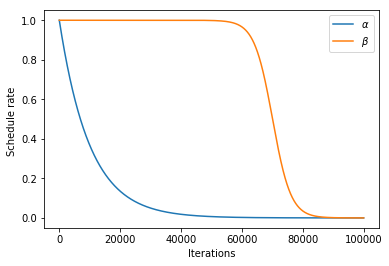
Figure 1: The schedule sampling rate for $\alpha$ and $\beta$

According to Bengio et al. (2015), we define the schedule rate $\alpha^{(i)}=k^{i}$ (where $0<k<1$, $i$ is the $i$th training iteration), and $\beta^{(i)}=k/(k+exp(i/k))$ (where $k>1$, $i$ is the $i$th training iteration). In the experiments shown in Tabel 1, for the schedule rate $\alpha$, we set $k=0.9999$; for the schedule rate $\beta$, we set $k=3000$, and the resulting schedule rate curve is shown in Figure 1.

Appendix B Additional Results

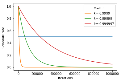
Figure 2: The schedule rate $\alpha$ in Dagger

We try different schedule rate settings in Dagger as shown in Figure 2, and compare their model performances on both datasets. The corresponding experimental results are shown in Table 3 and Table 4 respectively.

We find that if $\alpha$ decreases faster ($k=0.9999$) than the model convergence speed, the model will stop improving before it learns the optimal policy; if $\alpha$ decreases slower ($k=0.999997$) than the model convergence speed, the model will get stuck in the sub-optimal policy.

For the Quora dataset, we find our model learns the optimal policy when it gets half chance to take the ground truth word $y_{t-1}$ as $\tilde{y}_{t-1}$ (i.e. the schedule rate setting is $\alpha=0.5$ and $\beta=1$).

For the twitter dataset, we find our model learns the optimal policy when it has higher probability to take the decoded word $\hat{y}_{t-1}$ as $\tilde{y}_{t-1}$ (i.e. the schedule rate setting is $\alpha=0.2$ and $\beta=1$).

References

- Bagnell et al. (2007) JA Bagnell, Joel Chestnutt, David M Bradley, and Nathan D Ratliff. 2007. Boosting structured prediction for imitation learning. In Advances in Neural Information Processing Systems, pages 1153–1160.
- Bahdanau et al. (2016) Dzmitry Bahdanau, Philemon Brakel, Kelvin Xu, Anirudh Goyal, Ryan Lowe, Joelle Pineau, Aaron Courville, and Yoshua Bengio. 2016. An actor-critic algorithm for sequence prediction. arXiv preprint arXiv:1607.07086.
- Bahdanau et al. (2014) Dzmitry Bahdanau, Kyunghyun Cho, and Yoshua Bengio. 2014. Neural machine translation by jointly learning to align and translate. arXiv preprint arXiv:1409.0473.
- Barzilay and Lee (2003) Regina Barzilay and Lillian Lee. 2003. Learning to paraphrase: An unsupervised approach using multiple-sequence alignment. In Proceedings of the 2003 Conference of the North American Chapter of the Association for Computational Linguistics on Human Language Technology - Volume 1, NAACL ’03, pages 16–23, Stroudsburg, PA, USA. Association for Computational Linguistics.
- Barzilay and McKeown (2001) Regina Barzilay and Kathleen R McKeown. 2001. Extracting paraphrases from a parallel corpus. In Proceedings of the 39th annual meeting of the Association for Computational Linguistics.
- Bengio et al. (2015) Samy Bengio, Oriol Vinyals, Navdeep Jaitly, and Noam Shazeer. 2015. Scheduled sampling for sequence prediction with recurrent neural networks. In Advances in Neural Information Processing Systems, pages 1171–1179.
- Buck et al. (2017) Christian Buck, Jannis Bulian, Massimiliano Ciaramita, Wojciech Gajewski, Andrea Gesmundo, Neil Houlsby, and Wei Wang. 2017. Ask the right questions: Active question reformulation with reinforcement learning. arXiv preprint arXiv:1705.07830.
- Chang et al. (2015) Kai-Wei Chang, Akshay Krishnamurthy, Alekh Agarwal, Hal Daumé III, and John Langford. 2015. Learning to search better than your teacher. arXiv preprint arXiv:1502.02206.
- Chen and Bansal (2018) Yen-Chun Chen and Mohit Bansal. 2018. Fast abstractive summarization with reinforce-selected sentence rewriting. arXiv preprint arXiv:1805.11080.
- Cho et al. (2015) Kyunghyun Cho, Aaron Courville, and Yoshua Bengio. 2015. Describing multimedia content using attention-based encoder-decoder networks. IEEE Transactions on Multimedia, 17(11):1875–1886.
- Cho et al. (2014) Kyunghyun Cho, Bart Van Merriënboer, Caglar Gulcehre, Dzmitry Bahdanau, Fethi Bougares, Holger Schwenk, and Yoshua Bengio. 2014. Learning phrase representations using rnn encoder-decoder for statistical machine translation. arXiv preprint arXiv:1406.1078.
- Chopra et al. (2016) Sumit Chopra, Michael Auli, and Alexander M Rush. 2016. Abstractive sentence summarization with attentive recurrent neural networks. In Proceedings of the 2016 Conference of the North American Chapter of the Association for Computational Linguistics: Human Language Technologies, pages 93–98.
- Daumé et al. (2009) Hal Daumé, John Langford, and Daniel Marcu. 2009. Search-based structured prediction. Machine learning, 75(3):297–325.
- Dayan and Niv (2008) Peter Dayan and Yael Niv. 2008. Reinforcement learning: the good, the bad and the ugly. Current opinion in neurobiology, 18(2):185–196.
- Dong et al. (2017) Li Dong, Jonathan Mallinson, Siva Reddy, and Mirella Lapata. 2017. Learning to paraphrase for question answering. arXiv preprint arXiv:1708.06022.
- Ibrahim et al. (2003) Ali Ibrahim, Boris Katz, and Jimmy Lin. 2003. Extracting structural paraphrases from aligned monolingual corpora. In Proceedings of the second international workshop on Paraphrasing-Volume 16, pages 57–64.
- Keneshloo et al. (2018) Yaser Keneshloo, Tian Shi, Naren Ramakrishnan, and Chandan K. Reddy. 2018. Deep reinforcement learning for sequence to sequence models. arXiv preprint arXiv:1805.09461.
- Lan et al. (2017) Wuwei Lan, Siyu Qiu, Hua He, and Wei Xu. 2017. A continuously growing dataset of sentential paraphrases. In Proceedings of the 2017 Conference on Empirical Methods in Natural Language Processing, pages 1224–1234, Copenhagen, Denmark. Association for Computational Linguistics.
- Li et al. (2018) Zichao Li, Xin Jiang, Lifeng Shang, and Hang Li. 2018. Paraphrase generation with deep reinforcement learning. In Proceedings of the 2018 Conference on Empirical Methods in Natural Language Processing.
- Lin (2004) Chin-Yew Lin. 2004. Rouge: A package for automatic evaluation of summaries. Text Summarization Branches Out.
- Liu et al. (2018) Ming Liu, Wray Buntine, and Gholamreza Haffari. 2018. Learning how to actively learn: A deep imitation learning approach. In Proceedings of the 56th Annual Meeting of the Association for Computational Linguistics (Volume 1: Long Papers), pages 1874–1883.
- Madnani et al. (2007) Nitin Madnani, Necip Fazil Ayan, Philip Resnik, and Bonnie J Dorr. 2007. Using paraphrases for parameter tuning in statistical machine translation. In Proceedings of the Second Workshop on Statistical Machine Translation, pages 120–127. Association for Computational Linguistics.
- Mallinson et al. (2017) Jonathan Mallinson, Rico Sennrich, and Mirella Lapata. 2017. Paraphrasing revisited with neural machine translation. In Proceedings of the 15th Conference of the European Chapter of the Association for Computational Linguistics: Volume 1, Long Papers, pages 881–893.
- McCann et al. (2018) Bryan McCann, Nitish Shirish Keskar, Caiming Xiong, and Richard Socher. 2018. The natural language decathlon: Multitask learning as question answering. arXiv preprint arXiv:1806.08730.
- Pang et al. (2003) Bo Pang, Kevin Knight, and Daniel Marcu. 2003. Syntax-based alignment of multiple translations: Extracting paraphrases and generating new sentences. In Proceedings of the 2003 Conference of the North American Chapter of the Association for Computational Linguistics on Human Language Technology-Volume 1, pages 102–109.
- Papineni et al. (2002) Kishore Papineni, Salim Roukos, Todd Ward, and Wei-Jing Zhu. 2002. Bleu: a method for automatic evaluation of machine translation. In Proceedings of the 40th annual meeting on association for computational linguistics, pages 311–318. Association for Computational Linguistics.
- Patro et al. (2018) Badri N Patro, Vinod K Kurmi, Sandeep Kumar, and Vinay P Namboodiri. 2018. Learning semantic sentence embeddings using pair-wise discriminator. arXiv preprint arXiv:1806.00807.
- Prakash et al. (2016) Aaditya Prakash, Sadid A Hasan, Kathy Lee, Vivek Datla, Ashequl Qadir, Joey Liu, and Oladimeji Farri. 2016. Neural paraphrase generation with stacked residual LSTM networks. arXiv preprint arXiv:1610.03098.
- Quirk et al. (2004) Chris Quirk, Chris Brockett, and William Dolan. 2004. Monolingual machine translation for paraphrase generation. In Proceedings of the 2004 conference on empirical methods in natural language processing, pages 142–149.
- Radford et al. (2019) Alec Radford, Jeffrey Wu, Rewon Child, David Luan, Dario Amodei, and Ilya Sutskever. 2019. Language models are unsupervised multitask learners. OpenAI Blog, 1:8.
- Ranzato et al. (2015) Marc’Aurelio Ranzato, Sumit Chopra, Michael Auli, and Wojciech Zaremba. 2015. Sequence level training with recurrent neural networks. arXiv preprint arXiv:1511.06732.
- Ross et al. (2011) Stéphane Ross, Geoffrey Gordon, and Drew Bagnell. 2011. A reduction of imitation learning and structured prediction to no-regret online learning. In Proceedings of the fourteenth international conference on artificial intelligence and statistics, pages 627–635.
- See et al. (2017) Abigail See, Peter J Liu, and Christopher D Manning. 2017. Get to the point: Summarization with pointer-generator networks. arXiv preprint arXiv:1704.04368.
- Shen et al. (2015) Shiqi Shen, Yong Cheng, Zhongjun He, Wei He, Hua Wu, Maosong Sun, and Yang Liu. 2015. Minimum risk training for neural machine translation. arXiv preprint arXiv:1512.02433.
- Vlachos (2013) Andreas Vlachos. 2013. An investigation of imitation learning algorithms for structured prediction. In European Workshop on Reinforcement Learning, pages 143–154.
- Williams (1992) Ronald J Williams. 1992. Simple statistical gradient-following algorithms for connectionist reinforcement learning. Machine learning, 8(3-4):229–256.
- Wu et al. (2018) Lijun Wu, Fei Tian, Tao Qin, Jianhuang Lai, and Tie-Yan Liu. 2018. A study of reinforcement learning for neural machine translation. arXiv preprint arXiv:1808.08866.
- Yin et al. (2018) Qingyu Yin, Yu Zhang, Weinan Zhang, Ting Liu, and William Yang Wang. 2018. Deep reinforcement learning for chinese zero pronoun resolution. arXiv preprint arXiv:1806.03711.
- Zhao et al. (2009) Shiqi Zhao, Xiang Lan, Ting Liu, and Sheng Li. 2009. Application-driven statistical paraphrase generation. In Proceedings of the Joint Conference of the 47th Annual Meeting of the ACL and the 4th International Joint Conference on Natural Language Processing of the AFNLP: Volume 2 - Volume 2, ACL ’09, pages 834–842, Stroudsburg, PA, USA. Association for Computational Linguistics.