1 Introduction

The decay of the false vacua is an important phenomenon in particle physics and cosmology. The lifetime of the false vacua can be calculated by the Euclidean path integral [3]. (For an earlier work, see Ref. [4, 5].) In this formalism, the bounce solution which is a saddle point of the action gives the dominant contribution to the decay width. There exist several numerical packages to calculate the bounce solution; CosmoTransitions [6, 7], AnyBubble [8], and BubbleProfiler [9, 10]. For other numerical algorithms, see Refs. [11, 12, 13, 14, 15, 16, 17, 18, 19, 20, 21, 22, 23].

In this paper, we introduce a new numerical package to calculate the bounce solution. Our package utilizes a gradient flow equation. This framework is recently proposed by Chigusa, Moroi, and Shoji [24]. Our package solves a flow equation which is proposed by the author [1]. As we will see in the next section, our flow equation minimizes the kinetic energy of configuration while fixing the potential energy. Thanks to Coleman–Glaser–Martin’s discussion [2], the bounce solution is obtained by a scale transformation of the fixed point of the flow equation.

2 Formulation

Here we briefly summarize the gradient flow equation which is proposed in Ref. [1].

We take the Euclidean action with $n_{\phi}$ scalar fields which have the canonical kinetic term and a generic potential term:

$${\cal S}_{E}[\phi]={\cal T}[\phi]+{\cal V}[\phi],\qquad{\cal T}[\phi]=\sum_{i=1}^{n_{\phi}}\int d^{d}x\frac{1}{2}(\nabla\phi_{i})^{2},\qquad{\cal V}[\phi]=\int d^{d}x[V(\phi)-V(\phi_{FV})].$$ (1)

Here $d$ is the dimension of the Euclidean space, and we assume $d$ is larger than 2. The scalar potential $V$ satisfies $\partial V/\partial\phi_{i}|_{\phi=\phi_{FV}}=0$, all of the eigenvalues of the Hessian of $V$ at $\phi_{i}=\phi_{FV,i}$ are non-negative, and $V(\phi)-V(\phi_{FV})$ is somewhere negative. The bounce solution is a configuration which satisfies the following equation of motion and the boundary condition at infinity:

$$-\nabla^{2}\phi_{i}+\frac{\partial V}{\partial\phi_{i}}=0,\qquad\lim_{|x|\to\infty}\phi_{i}(x)=\phi_{FV,i}.$$ (2)

The bounce solution has $O(d)$ symmetry [2, 25, 26, 27] in the space. Thus, the equation of motion can be simplified as

$$-\frac{d^{2}\phi_{i}}{dr^{2}}-\frac{d-1}{r}\frac{d\phi_{i}}{dr}+\frac{\partial V}{\partial\phi_{i}}=0.$$ (3)

Here we solve the minimization problem of the kinetic energy ${\cal T}[\phi]$ while fixing the negative potential energy ${\cal V}[\phi]<0$ rather than solving the above equation of motion directly. This is the reduced problem of the bounce solution which is proposed in Ref. [2]. The solution of this problem is a scale-transformed of the bounce solution. In Ref. [1], a gradient flow equation is proposed to solve this problem. We introduce functions $\varphi_{i}(r,\tau)$ and the flow of $\varphi$ is described as

$$\frac{\partial}{\partial\tau}\varphi_{i}(r,\tau) =\nabla^{2}\varphi_{i}-\lambda[\varphi]\frac{\partial V(\varphi)}{\partial\varphi_{i}},$$ (4)

$$\lambda[\varphi] =\frac{\displaystyle\sum_{i=1}^{n_{\phi}}\int_{0}^{\infty}drr^{d-1}\frac{\partial V(\varphi)}{\partial\varphi_{i}}\nabla^{2}\varphi_{i}}{\displaystyle\sum_{i=1}^{n_{\phi}}\int_{0}^{\infty}drr^{d-1}\left(\frac{\partial V(\varphi)}{\partial\varphi_{i}}\right)^{2}}.$$ (5)

Note that $\lambda[\varphi]$ depends on $\tau$ but not on $r$. Here $\tau$ is “time” for the flow of $\varphi$ and $\nabla^{2}\varphi_{i}=\partial_{r}^{2}\varphi_{i}+(d-1)(\partial_{r}\varphi)/r$. We take the initial $\varphi(r,0)$ such that

$${\cal V}[\varphi]|_{\tau=0}<0.$$ (6)

We can easily check

$$\frac{d}{d\tau}{\cal V}[\varphi]=0,\qquad\frac{d}{d\tau}{\cal T}[\varphi]\leq 0.$$ (7)

For details, see Ref. [1]. In the limit of large $\tau$, $\varphi$ reaches a fixed point and satisfies $\nabla^{2}\varphi-\lambda[\varphi](\partial V/\partial\varphi)=0$. This fixed point is not a saddle point because we fixed ${\cal V}$, and this property guarantees the stability of numerical calculation. The bounce solution $\phi_{B}$ can be obtained by the following scale transformation of the fixed point $\varphi$.

$$\phi_{B}(r)=\lim_{\tau\to\infty}\varphi(\lambda^{1/2}r,\tau).$$ (8)

Note that ${\cal V}[\phi_{B}]<0$ is guaranteed thanks to Eq. (6) and Eq. (7) and $\phi_{B}$ is a configuration which is relevant with the false vacuum decay.

3 Algorithm

We solve the flow equation Eq. (4) numerically. We discretize $r$-space and take $n$ points at $r_{i}=(i-1)\delta r$ for $i=1,\cdots,n$. The radius of the sphere is $R\equiv(n-1)\delta r$, however, the value of $R$ itself is not important because we utilize the scale transformation property of the bounce solution. We take the following discretized Laplacian which is similar to Ref. [28]:

$$\nabla^{2}\varphi_{i}|_{r=r_{j}}=\left(\frac{d^{2}\varphi_{i}}{dr^{2}}+\frac{d-1}{r}\frac{d\varphi_{i}}{dr}\right)_{r=r_{j}}=\begin{cases}\displaystyle\frac{2d(\varphi_{i,2}-\varphi_{i,1})}{\delta r^{2}}&(j=1)\\[11.38109pt] \displaystyle\frac{\varphi_{i,j+1}-2\varphi_{i,j}+\varphi_{i,j-1}}{\delta r^{2}}+\frac{d-1}{r_{j}}\frac{\varphi_{i,j+1}-\varphi_{i,j-1}}{2\delta r}&(j>1)\end{cases}$$ (9)

The integrals in Eq. (5) are approximated by the trapezoidal rule. We take a boundary condition such that $\varphi_{i,n}=\phi_{FV,i}$.

Each step of the evolution of $\varphi$ is evaluated as

$$\varphi_{i}(r,\tau+\delta\tau)=\delta\tau\times\left[\nabla^{2}\varphi_{i}-\lambda[\varphi]\frac{\partial V(\varphi)}{\partial\varphi_{i}}\right].$$ (10)

We repeat this evolution until $\varphi$ converges. For the stability of the numerical calculation, $\delta\tau$ should be ${\cal O}(\delta r^{2})$ otherwise the fluctuation with large wave number exponentially grows.

We take the following configuration as the initial condition.

$$\varphi_{i}(r,0)=\phi_{TV,i}+\frac{1}{2}(\phi_{FV,i}-\phi_{TV,i})\left(1+\tanh\left(\frac{r_{i}-r_{0}}{\sigma}\right)\right).$$ (11)

Here $\phi_{TV}$ is chosen such that $V(\phi_{TV})<V(\phi_{FV})$. (Note that $\phi_{TV}$ is not necessarily to be the true vacuum. Also the algorithm presented here works even there exists no true vacuum. For example, Ref. [1] shows this algorithm works with $V(\phi)=\phi^{2}/2-\phi^{3}/3$.) The initial $r_{0}$ is set to some value which is smaller than $R$ ($0.5R$ as default), and $\sigma$ is set to be sufficiently small to obtain negative ${\cal V}$. In order to satisfy the boundary condition at infinity, the first derivative of the field should be small enough. If $\partial\phi_{i}/\partial r|_{r=R}=(\phi_{i,n}-\phi_{i,n-1})/\delta r$ is not small after solving the flow equation, the size of the bounce is not small enough compared to the size of the space $R$. In this case, we solve the flow equation again with smaller $r_{0}$. See also Fig. 1.

Figure 1: Flow chart of the algorithm of SimpleBounce. The default values of $\tau_{0}$ and $\tau_{1}$ are 0.05 and 0.4.

4 User instructions

This package is available at https://github.com/rsato64/SimpleBounce. The main files are simplebounce.cc and simplebounce.h. The sample executable files are compiled by

make

The default compiler is g++. If you need to change this, please edit Makefile.inc. In this package, the following examples are available.

• sample1.x
  This calculates the Euclidean action for the bounce in a single scalar field model. See also section 5.1.

• benchmark/compare_with_cosmotransitions/
  run_simplebounce.sh in this folder gives Tab. 1. See also section 5.2.

• benchmark/change_n_tau/
  run.sh in this folder gives Fig. 2. See also section 5.3.

5 Sample codes and discussions

Here we describe several sample codes and discuss their results.

5.1 Sample code for single scalar field model

Here we show an example of code. The following information is required to calculate the bounce solution:

• The number of scalar field $n_{\phi}$

• The scalar potential $V(\phi)$

• The first derivative(s) of the scalar potential $\partial V/\partial\phi_{i}$

• The position of the false vacuum $\phi_{FV}$

• A point $\phi_{TV}$ which gives $V(\phi_{TV})<V(\phi_{FV})$.

Here we take the potential as

$$V(\phi)=\frac{1}{2}\phi^{2}-\frac{1}{3}\phi^{3}.$$ (12)

The false vacuum is at $\phi=0$. The scalar field $\phi$ will tunnel into positive $\phi$ region. The source file sample1.cc is given as

⬇

#include<iostream>

#include"simplebounce.h"

using namespace std;

using namespace simplebounce;

class MyModel : public GenericModel{

public:

MyModel(){

setNphi(1); // number of scalar field(s)

}

// potential for scalar field(s)

double vpot (const double* phi) const{

return phi[0]*phi[0]/2. - phi[0]*phi[0]*phi[0]/3.;

}

// first derivative(s) of potential

void calcDvdphi(const double *phi) const{

dvdphi[0] = phi[0] - phi[0]*phi[0];

}

};

int main() {

BounceCalculator bounce;

bounce.verboseOn(); // verbose mode

bounce.setRmax(1.); // phi(rmax) = phi(False vacuum)

bounce.setDimension(4); // number of space dimension

bounce.setN(100); // number of grid

MyModel model;

bounce.setModel(&model);

double phiTV[1] = {10.}; // a point at which V<0

double phiFV[1] = {0.}; // false vacuum

bounce.setVacuum(phiTV, phiFV);

// calcualte the bounce solution

bounce.solve();

// show the results

bounce.printBounce();

// show the Euclidean action

cout << "S_E = " << bounce.action() << endl;

return 0;

}

Then, the executable file can be generated by, for example, g++ sample1.cc simplebounce.cc -O3.

5.2 The Euclidean action for benchmark models

Tab. 1 shows the Euclidean action and the runtime for several benchmark models, which are taken from Refs. [10, 24]. We also show the results and runtimes by CosmoTransitions in the table. We can see the results of our package agree with CosmoTransitions, and our package is faster for the benchmark models. We can expect the running time is proportional to the number of the scalar field because the code calculates Eq. (10) and Eq. (5) at each time step. Tab. 1 is roughly consistent with this expectation.

	${\cal S}_{E}$		Time[s]
model	SB	CT	SB	CT
#1 in Tab. 1 of [10]	$52.4$	$52.6$	0.04	0.05
#2 in Tab. 1 of [10]	$20.8$	$21.1$	0.04	0.35
#3 in Tab. 1 of [10]	$22.0$	$22.0$	0.07	0.17
#4 in Tab. 1 of [10]	$55.8$	$56.1$	0.07	0.31
#5 in Tab. 1 of [10]	$16.2$	$16.4$	0.09	0.26
#6 in Tab. 1 of [10]	$24.4$	$24.5$	0.11	0.25
#7 in Tab. 1 of [10]	$36.6$	$36.7$	0.14	0.22
#8 in Tab. 1 of [10]	$45.9$	$46.1$	0.16	0.23
Eq. 40 of [24]	$1.08\times 10^{3}$	$1.09\times 10^{3}$	0.03	0.09
Eq. 41 of [24]	$6.62$	$6.65$	0.03	0.06
Eq. 42 of [24]	$1.75\times 10^{3}$	$1.77\times 10^{3}$	0.34	0.54
Eq. 43 of [24]	$4.45$	$4.50$	0.05	0.19

Table 1: The comparison with CosmoTransitions. For CosmoTransitions, we take fRatioConv as 0.02. The bounce action ${\cal S}_{E}$ is calculated for $d=3$. The runtimes are measured by Thinkpad X250 with Ubuntu 16.04, whose CPU is Intel®Core™i7-5600U (2.60 GHz) and compiler is GCC version 5.4.0. We take -O3 as the optimization option.

5.3 Changing $n$ and $\tau_{1}$

In Fig. 2, we show the value of ${\cal S}_{E}$ for different number of the lattice $n$ and the flow time $\tau_{1}$. We can see that the value of ${\cal S}_{E}$ converges for large $n$ and large $\tau_{1}$, and we can get the result of ${\cal O}(0.1)~{}\%$ accuracy in ${\cal O}(0.1)$ s run with $n=100$. Fig. 2 also shows that the runtime is proportional to $n^{3}$. This is because the step $\delta\tau$ is bounded as $\sim\delta r^{2}$. Thus, in general, thin wall bounce takes much more time than thick wall bounce to obtain accurate result.

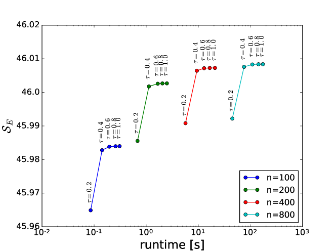
Figure 2: The runtime of the value of ${\cal S}_{E}$ for different number of the lattice $n$ and the flow time $\tau_{1}$. We take the model #8 in Tab. 1 of [10]. The environment of PC is same as Tab. 1.

References

- [1] R. Sato, “Simple Gradient Flow Equation for the Bounce Solution,” Phys. Rev. D 101 no. 1, (2020) 016012, arXiv:1907.02417 [hep-ph].
- [2] S. R. Coleman, V. Glaser, and A. Martin, “Action Minima Among Solutions to a Class of Euclidean Scalar Field Equations,” Commun. Math. Phys. 58 (1978) 211–221.
- [3] S. R. Coleman, “The Fate of the False Vacuum. 1. Semiclassical Theory,” Phys. Rev. D15 (1977) 2929–2936. [Erratum: Phys. Rev.D16,1248(1977)].
- [4] T. D. Lee and G. C. Wick, “Vacuum Stability and Vacuum Excitation in a Spin 0 Field Theory,” Phys. Rev. D9 (1974) 2291–2316.
- [5] P. H. Frampton, “Vacuum Instability and Higgs Scalar Mass,” Phys. Rev. Lett. 37 (1976) 1378. [Erratum: Phys. Rev. Lett.37,1716(1976)].
- [6] S. Profumo, L. Ubaldi, and C. Wainwright, “Singlet Scalar Dark Matter: monochromatic gamma rays and metastable vacua,” Phys. Rev. D82 (2010) 123514, arXiv:1009.5377 [hep-ph].
- [7] C. L. Wainwright, “CosmoTransitions: Computing Cosmological Phase Transition Temperatures and Bubble Profiles with Multiple Fields,” Comput. Phys. Commun. 183 (2012) 2006–2013, arXiv:1109.4189 [hep-ph].
- [8] A. Masoumi, K. D. Olum, and B. Shlaer, “Efficient numerical solution to vacuum decay with many fields,” JCAP 1701 no. 01, (2017) 051, arXiv:1610.06594 [gr-qc].
- [9] S. Akula, C. Balázs, and G. A. White, “Semi-analytic techniques for calculating bubble wall profiles,” Eur. Phys. J. C76 no. 12, (2016) 681, arXiv:1608.00008 [hep-ph].
- [10] P. Athron, C. Balázs, M. Bardsley, A. Fowlie, D. Harries, and G. White, “BubbleProfiler: finding the field profile and action for cosmological phase transitions,” Comput. Phys. Commun. 244 (2019) 448–468, arXiv:1901.03714 [hep-ph].
- [11] M. Claudson, L. J. Hall, and I. Hinchliffe, “Low-Energy Supergravity: False Vacua and Vacuous Predictions,” Nucl. Phys. B228 (1983) 501–528.
- [12] A. Kusenko, “Improved action method for analyzing tunneling in quantum field theory,” Phys. Lett. B358 (1995) 51–55, arXiv:hep-ph/9504418 [hep-ph].
- [13] A. Kusenko, P. Langacker, and G. Segre, “Phase transitions and vacuum tunneling into charge and color breaking minima in the MSSM,” Phys. Rev. D54 (1996) 5824–5834, arXiv:hep-ph/9602414 [hep-ph].
- [14] J. M. Moreno, M. Quiros, and M. Seco, “Bubbles in the supersymmetric standard model,” Nucl. Phys. B526 (1998) 489–500, arXiv:hep-ph/9801272 [hep-ph].
- [15] J. M. Cline, J. R. Espinosa, G. D. Moore, and A. Riotto, “String mediated electroweak baryogenesis: A Critical analysis,” Phys. Rev. D59 (1999) 065014, arXiv:hep-ph/9810261 [hep-ph].
- [16] P. John, “Bubble wall profiles with more than one scalar field: A Numerical approach,” Phys. Lett. B452 (1999) 221–226, arXiv:hep-ph/9810499 [hep-ph].
- [17] J. M. Cline, G. D. Moore, and G. Servant, “Was the electroweak phase transition preceded by a color broken phase?,” Phys. Rev. D60 (1999) 105035, arXiv:hep-ph/9902220 [hep-ph].
- [18] T. Konstandin and S. J. Huber, “Numerical approach to multi dimensional phase transitions,” JCAP 0606 (2006) 021, arXiv:hep-ph/0603081 [hep-ph].
- [19] J.-h. Park, “Constrained potential method for false vacuum decays,” JCAP 1102 (2011) 023, arXiv:1011.4936 [hep-ph].
- [20] V. Guada, A. Maiezza, and M. Nemevšek, “Multifield Polygonal Bounces,” Phys. Rev. D99 no. 5, (2019) 056020, arXiv:1803.02227 [hep-th].
- [21] R. Jinno, “Machine learning for bounce calculation,” arXiv:1805.12153 [hep-th].
- [22] J. R. Espinosa and T. Konstandin, “A Fresh Look at the Calculation of Tunneling Actions in Multi-Field Potentials,” JCAP 1901 no. 01, (2019) 051, arXiv:1811.09185 [hep-th].
- [23] M. L. Piscopo, M. Spannowsky, and P. Waite, “Solving differential equations with neural networks: Applications to the calculation of cosmological phase transitions,” Phys. Rev. D100 no. 1, (2019) 016002, arXiv:1902.05563 [hep-ph].
- [24] S. Chigusa, T. Moroi, and Y. Shoji, “Bounce Configuration from Gradient Flow,” Phys. Lett. B 800 (2020) 135115, arXiv:1906.10829 [hep-ph].
- [25] O. Lopes, “Radial symmetry of minimizers for some translation and rotation invariant functionals,” Journal of differential equations 124 no. 2, (1996) 378–388.
- [26] J. Byeon, L. Jeanjean, and M. Mariş, “Symmetry and monotonicity of least energy solutions,” Calculus of Variations and Partial Differential Equations 36 no. 4, (2009) 481–492, arXiv:0806.0299 [math.AP].
- [27] K. Blum, M. Honda, R. Sato, M. Takimoto, and K. Tobioka, “O() Invariance of the Multi-Field Bounce,” JHEP 05 (2017) 109, arXiv:1611.04570 [hep-th]. [Erratum: JHEP06,060(2017)].
- [28] N. Bar, K. Blum, J. Eby, and R. Sato, “Ultralight dark matter in disk galaxies,” Phys. Rev. D99 no. 10, (2019) 103020, arXiv:1903.03402 [astro-ph.CO].