Observations of Electromagnetic Electron Holes and Evidence of Cherenkov Whistler Emission

Abstract

We report observations of electromagnetic electron holes (EHs). We use multi-spacecraft analysis to quantify the magnetic field contributions of three mechanisms: the Lorentz transform, electron drift within the EH, and Cherenkov emission of whistler waves. The first two mechanisms account for the observed magnetic fields for slower EHs, while for EHs with speeds approaching half the electron Alfvén speed, whistler waves excited via the Cherenkov mechanism dominate the perpendicular magnetic field. The excited whistlers are kinetically damped and typically confined within the EHs.

Electron holes (EHs) are localized nonlinear plasma structures in which electrons are self-consistently trapped by a positive potential [1, 2, 3]. By scattering and heating electrons, EHs play an important part in plasma dynamics [4, 5]. EHs are frequently observed in space [6, 7, 8, 9, 10] and laboratory [11, 12, 13] plasmas. They are typically manifested in data as diverging, bipolar, electric fields parallel to the ambient magnetic field. EHs are formed by various instabilities [14, 15], and are thus indicators of prior instability and turbulence. Their connection with streaming instabilities leads them to frequently appear during magnetic reconnection [16, 17, 18, 19]. Furthermore, simulations of magnetic reconnection have shown EHs can Cherenkov radiate whistler waves which in turn affect the reconnection rate [20]. Studying EHs can thus prove important for understanding key plasma phenomena such as magnetic reconnection.

Though EHs are usually considered electrostatic, observations of electromagnetic EHs have been made in Earth’s magnetotail [21, 22]. The observed magnetic fields ($\delta\mathbf{B}$) were argued to be the sum of two independent fields. First, $\delta\mathbf{B}_{L}$ generated by the Lorentz transform, of the electrostatic field, and second, $\delta\mathbf{B}_{d}$ generated by the $\delta\mathbf{E}\times\mathbf{B}_{0}$ drift of electrons associated with the EH electric field and ambient magnetic field [21, 23]. These studies were limited either by the fact that the EHs were only observed at one point in space [21], or provided only estimates of $\delta B_{d\parallel}$ at the EH center [22]. With the Magnetospheric Multiscale (MMS) [24] mission, it is possible to use four-spacecraft measurements to obtain a complete three-dimensional description of EHs [25, 26, 27], enabling $\delta\mathbf{B}$ to be investigated in greater detail [25].

In this letter we use data from MMS to investigate electromagnetic EHs frequently observed during boundary layer crossings in the magnetotail. We use multi-spacecraft methods to quantify different contributions to $\delta\mathbf{B}$. Our results show that $\delta B_{d,\parallel}$ well explains the observed $\delta B_{\parallel}$, and that $\delta\mathbf{B}_{d,\perp}$ is in good agreement with observations for EHs that are much slower than the electron Alfvén speed. For increasing EH speeds we show, for the first time, that localized whistler waves are excited from the EHs via the Cherenkov mechanism and contribute significantly to $\delta\mathbf{B}_{\perp}$.

Fig. 1 shows an example of a plasma sheet boundary layer crossing containing signatures of magnetic reconnection and EHs with magnetic fields.

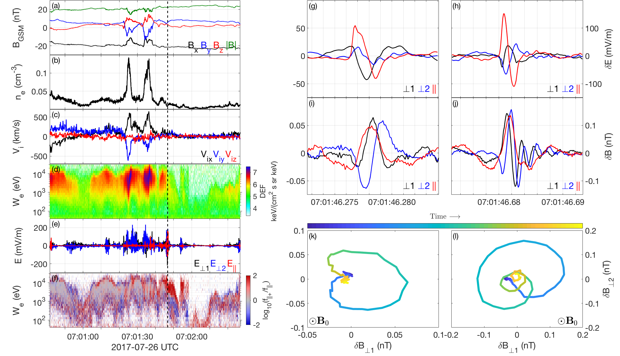
Figure 1: Left: Event overview. (a) Magnetic field from FGM [28] in geocentric solar magnetospheric (GSM) coordinates, (b) plasma density from FPI [29], (c) ion velocity from FPI in GSM, (d) electron energy spectrogram from FPI, (e) electric field from EDP [30, 31] in field-aligned coordinates, (f) spectrogram of the ratio of the parallel and anti-parallel electron phase-space density from FPI. The vertical dashed line shows where EHs are observed. Right: Examples of electromagnetic EHs. The data is high-pass filtered at 100 Hz. (g,h) Electric field from EDP, (i,j) magnetic field from SCM [32], (k,l) hodograms of $\delta\mathbf{B}_{\perp}$.

At 2017-07-26 07:00 UT, MMS was in the plasma sheet and detected a fast reconnection jet moving tailward (Fig. 1c). At 07:01:30, the ion flow reversed, and MMS entered the boundary layer between the plasma sheet and the tail lobes (Fig. 1d) where strong wave activity was observed (Fig. 1e). First as low-frequency $E_{\perp}$ oscillations consistent with lower hybrid drift waves [33], and later as solitary $E_{\parallel}$ waves marked by the vertical dashed line in Fig. 1e, and exemplified in Figs. 1g,h. The solitary waves were accompanied by a high-energy electron beam (Fig. 1f) parallel to $\mathbf{B}_{0}$. By timing $E_{\parallel}$ between the spacecraft we find the structures to be EHs moving together with the beam. Notably the EHs have magnetic field fluctuations $\delta\mathbf{B}$ associated with them. We show two EH examples in Figs. 1g-j. While both EHs have positive and monopolar $\delta B_{\parallel}$ (distorted in the figure by high-pass filtering) confined within the EH, there are significant differences in $\delta\mathbf{B}_{\perp}$. For the first EH (Figs. 1g,i), $\delta\mathbf{B}_{\perp}$ is localized within the EH, whereas for the second EH, $\delta\mathbf{B}_{\perp}$ oscillates multiple times and forms a trailing tail (Fig. 1h,j). Note that of the roughly 40 EHs that were observed during this time, only two EHs had the tail-like feature in Fig. 1j, the others resembled Fig. 1i. The polarization of $\delta\mathbf{B}_{\perp}$ is right handed for all cases (Figs. 1k,l) with dominant frequency $\omega\approx 0.7\Omega_{ce}<\omega_{pe}$, where $\Omega_{ce}$ and $\omega_{pe}$ are the electron cyclotron and plasma frequencies.

We perform a statistical study to investigate how $\delta\mathbf{B}$ depends on EH properties. To accurately estimate the electron hole speed, $v_{EH}$, and parallel length scale, $l_{\parallel}$, the EHs should be detected by as many spacecraft as possible, and all four spacecraft are needed to accurately estimate the EH center potential, $\Phi_{0}$, and perpendicular length scale, $l_{\perp}$ [26, 27]. We therefore limit the study to June-August 2017, when MMS was probing the magnetotail with electron scale spacecraft separation. We take 9 data intervals where one or more groups of electromagnetic EHs are observed, resulting in a data-set of 336 EHs, all observed in connection to boundary layers similar to that in Fig. 1.

We use the multi-spacecraft timing method discussed in Ref. 27, cross-correlating $\delta E_{\parallel}$ between the spacecraft, to determine $\bm{v}_{EH}$, $l_{\parallel}$, and the measured potential $\Phi_{m}=\int{\delta E_{\parallel}v_{EH}dt}$ of the 336 EHs. The median propagation angle of the EHs with respect to $\mathbf{B}_{0}$ is 12^∘ which is within the uncertainty of the four-spacecraft timing, so $\bm{v}_{EH}$ is assumed to be field aligned. In Fig. 2 we plot $\Phi_{m}$ against $v_{EH}/v_{Ae}$ ($v_{Ae}=c\Omega_{ce}/\omega_{pe}$ is the electron Alfvén speed), with the peak value of $\delta\mathbf{B}_{\perp}$ color-coded. The figure shows that $\delta\mathbf{B}_{\perp}$ increases with potential and velocity. A dependence on $\Phi_{m}$ is expected since $\delta\mathbf{B}_{L},\delta\mathbf{B}_{d}\propto\delta\mathbf{E}_{\perp}\propto\Phi_{0}$ and the $v_{EH}/v_{Ae}$ dependence is qualitatively consistent with $\delta\mathbf{B}_{L}\propto v_{EH}$ since the EHs were observed in the same plasma region with, for the most part, similar $v_{Ae}$.

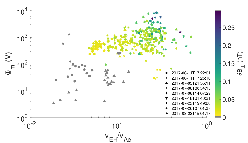
Figure 2: Measured EH potential $\Phi_{m}$ against $v_{EH}/v_{Ae}$ for 336 EHs, with the peak value of $\delta B_{\perp}$ color-coded. EHs from the same burst-data interval have the same symbol.

Next, we investigate the different mechanisms that can generate $\delta\mathbf{B}$. For weakly relativistic EHs (i.e. $\gamma\approx 1$) $\delta B_{L,\{\perp 1,\perp 2\}}=\mp v_{EH}\delta E_{\{\perp 2,\perp 1\}}/c^{2}$ [34]. By assuming the EH potential

$$\Phi(r,\theta,z)=\Phi_{0}e^{-r^{2}/2l_{\perp}^{2}}e^{-z^{2}/2l_{\parallel}^{2}},$$ (1)

$\delta\mathbf{B}_{d}$ is given by the Biot-Savart law of the $\delta\mathbf{E}\times\mathbf{B}_{0}$ current $J_{\theta}=en_{0}r\Phi(r,z)/(B_{0}l_{\perp}^{2})$ [23] as

$$\delta\mathbf{B}_{d}(\bm{x})=\frac{en_{0}\mu_{0}}{4\pi B_{0}}\int{\frac{r^{\prime}}{l_{\perp}^{2}}\Phi(r^{\prime},z^{\prime})\hat{\bm{\theta}}\times\frac{\bm{x}-\bm{x}^{\prime}}{|\bm{x}-\bm{x}^{\prime}|^{3}}d^{3}x^{\prime}},$$ (2)

where $n_{0}$ is the electron density, and $e$ is the elementary charge. In Fig. 3 we show two examples of EHs where we calculate and compare $\delta\mathbf{B}_{L}$ and $\delta\mathbf{B}_{d}$ with observations. The first EH (Figs. 3a-d) is small amplitude ($\Phi_{m}=680$ V), slow ($v_{EH}/v_{Ae}=1/9$) and has a weak $\delta\mathbf{B}\sim 0.01$ nT. We use the method of Ref. 26 (using, instead of the maximum value, $\delta\mathbf{E}_{\perp}$ evaluated at $\delta E_{\parallel}=0$) to fit the $\delta\mathbf{E}$ data of the four spacecraft to the electrostatic field corresponding to Eq. (1), giving $l_{\perp}=26$ km $=0.6d_{e}=1.6l_{\parallel}$, where $d_{e}=c/\omega_{pe}$ is the electron inertial length; $\Phi_{0}=915$ V $=1.4T_{e}/e$, where $T_{e}$ is the electron temperature; and the position of the EH. A representation of the fit is shown in Fig. 3a, where we plot the spacecraft (colored dots) and the EH (grey cross) position in the perpendicular plane. The arrows are the measured (colored) and predicted (grey) $\delta\mathbf{E}_{\perp}$ evaluated at $\delta E_{\parallel}=0$, showing that the EH fit well describes $\delta\mathbf{E}_{\perp}$ for all four spacecraft. A time series representation of the fit is shown in Fig. 3b for MMS4, where the measured and fitted $\delta\mathbf{E}$ are the solid and dashed lines respectively, affirming that the fit is in good agreement with observations. With $\Phi_{0}$, $l_{\parallel}$ and $l_{\perp}$ known, we solve Eq. (2) numerically to obtain $\delta\mathbf{B}_{d}$. $\delta\mathbf{B}_{L}$ is small, $|\delta\mathbf{B}_{L}|\approx 0.004$ nT. We plot MMS4 data of $\delta\mathbf{B}$ (solid) together with $\delta\mathbf{B}_{L}+\delta\mathbf{B}_{d}$ (dashed) in Fig. 3c, and the residual $\delta\mathbf{B}_{\text{Res}}=\delta\mathbf{B}-\delta\mathbf{B}_{L}-\delta\mathbf{B}_{d}$ in Fig. 3d. We find that $\delta\mathbf{B}\approx\delta\mathbf{B}_{d}$, the only discrepancy being that $|\delta B_{d,\perp 1}|$ is overestimated initially. This might be due to the fact that the EH has a steeper increase of $\delta E_{\parallel}$ than the model (Fig. 3b).

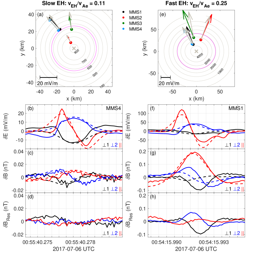
Figure 3: Two examples of EH fits and induced magnetic fields. (a) The position of MMS (colored dots) and the EH (grey cross) in the perpendicular plane. The measured and fitted $\delta\mathbf{E}_{\perp}$ are illustrated by the colored and grey arrows, respectively, where the arrow length is proportional to $|\delta\mathbf{E}_{\perp}|$. The grey contours are EH equipotential lines in Volts, and the magenta circle corresponds to $r=l_{\perp}$. (b) Measured (solid) and fitted (dashed) $\delta\mathbf{E}$. (c) Measured $\delta\mathbf{B}$ (solid) and calculated $\delta\mathbf{B}_{L}+\delta\mathbf{B}_{d}$ (dashed). (d) $\delta\mathbf{B}-\delta\mathbf{B}_{L}-\delta\mathbf{B}_{d}$. (e)-(h) Same format as (a)-(d) for a different EH. All fields are high-pass filtered at 50 Hz.

The second EH (Fig. 3e-h) has larger amplitude ($\Phi_{m}=3.5$ kV), is faster ($v_{EH}/v_{Ae}=1/4$) and has a stronger $\delta\mathbf{B}\sim 0.1$ nT. We perform the same analysis and present analogous plots in Fig. 3e-h. As before, the EH fit of $\delta\mathbf{E}$ (Fig. 3e,f) agrees well with observations ($\Phi_{0}=4.2$ kV $=1.9T_{e}/e$ and $l_{\perp}=40$ km $=1.1d_{e}=1.6l_{\parallel}$), $|\delta\mathbf{B}_{L}|\approx 0.02$ nT is small compared to $|\delta\mathbf{B}_{\perp}|$, and $\delta{B}_{\parallel}$ is well traced by $\delta B_{d,\parallel}$. However, when it comes to $\delta\mathbf{B}_{\perp}$ there is significant $\delta\mathbf{B}_{\text{Res},\perp}$ implying an additional mechanism is contributing to $\delta\mathbf{B}_{\perp}$. We note that $\delta\mathbf{B}_{\text{Res},\perp}$ is right hand polarized and its dominant frequency $f\approx 400$ Hz is below $f_{ce}\approx 650$ Hz. We estimate the wave normal angle of $\delta\mathbf{B}_{\text{Res},\perp}$ by $k_{\parallel}/k_{\perp}=\delta B_{\perp}/\delta B_{\parallel}=2.6$, corresponding to a wave normal angle $21^{\circ}$. We thus find that while $\delta\mathbf{B}$ of the slower EH can be fully explained by $\delta\mathbf{B}_{d}$, the faster EH has an additional $\delta\mathbf{B}_{\text{Res},\perp}$ with features consistent with whistler waves.

We are able to apply this method and calculate $\delta\mathbf{B}_{d}$ for a total of 19 EHs. The remaining EHs were either not observed by all four spacecraft ($\sim$50$\%$), had $\delta\mathbf{E}$ that was qualitatively inconsistent with the assumed potential model, e.g. bipolar $\delta\mathbf{E}_{\perp}$ ($\sim$25$\%$), or gave fitting results deemed too different from observations to be useful ($\sim$15$\%$). For these 19 EHs, $\delta B_{\parallel}$ is consistently well described by $\delta B_{d,\parallel}$, and $|\delta\mathbf{B}_{L}|\ll|\delta\mathbf{B}_{d,\perp}|$, meaning $\delta\mathbf{B}_{d}$ is more important for generating $\delta\mathbf{B}$ in the observed parameter range of Fig. 2. For all 19 EHs, when $\delta\mathbf{B}_{\text{Res},\perp}\neq 0$, it is right hand polarized with $\omega<\Omega_{ce}<\omega_{pe}$ which we interpret as being related to the whistler mode.

Because $\delta\mathbf{B}_{\text{Res},\perp}$ is localized to the EHs, we believe the EHs to be the source of the whistlers, rather than for example temperature anisotropy or Landau resonance. In fact, for most observations $T_{e\perp}/T_{e\parallel}<1$, so whistlers should not grow from temperature anisotropy. In this section we consider the generation of whistler waves from EHs via the Cherenkov mechanism, and show that this is consistent with our observations.

The theory of whistler waves Cherenkov emitted by EHs is developed and discussed in Ref. 20. In summary, the Cherenkov resonance condition is $\omega/k_{\parallel}=v_{EH}$ which specifies $\omega$ and $k_{\parallel}$ of the excited wave. Further, the ratio of the whistler electric field to that of the EH grows secularly (linearly in time) at a rate proportional to $(v_{EH}/v_{Ae})^{4}$, subject to $v_{EH}\leq v_{Ae}/2$.

To put our EH observations into the context of the Cherenkov mechanism, we plot the kinetic (orange and pink from WHAMP [35]) and cold (blue) whistler dispersion relation ($k_{\perp}=0$) for one group of slow EHs ($v_{EH}\approx v_{Ae}/16$) with $T_{\perp}/T_{\parallel}=1.0$ in Fig. 4a, and for one group of fast EHs ($v_{EH}\approx v_{Ae}/4$) with $T_{\perp}/T_{\parallel}=0.3$ in Fig. 4b. We define and plot $\omega_{EH}=\pi/t_{pp}$, where $t_{pp}$ is the peak-to-peak time of $\delta E_{\parallel}$, and $k_{EH}=\omega_{EH}/v_{EH}$, color-coding $\delta B_{\perp}$. The Cherenkov resonance condition is for a given EH manifested in the plots as the intersection of $\omega_{r}(k_{\parallel})$ with the straight line passing through the origin and the point $(k_{EH},\omega_{EH})$. The slope of this line corresponds to $v_{EH}$, meaning faster EHs excite whistlers with smaller $k_{\parallel}$. The shaded regions contain EH velocities between $\text{max}(v_{EH})$ and $\text{min}(v_{EH})$ for the two groups.

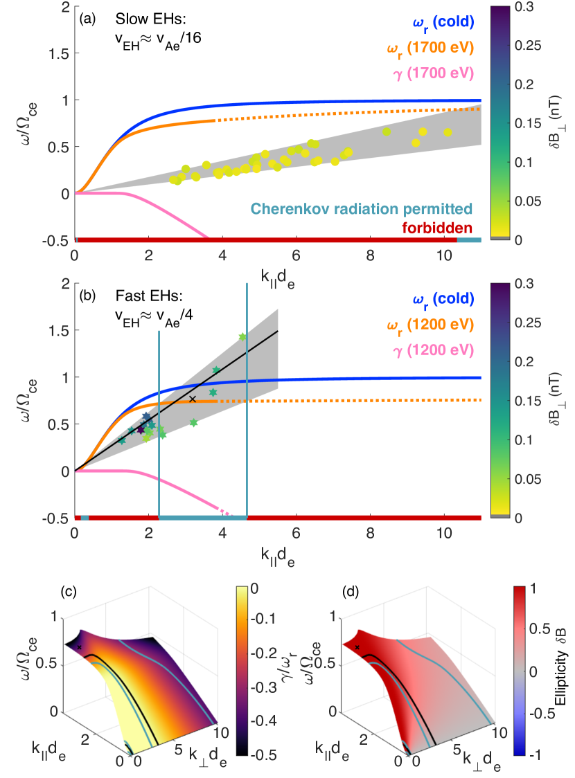
Figure 4: (a)-(b) Cold (blue) and kinetic (orange and pink) whistler dispersion relation ($k_{\perp}=0$) for two different groups of EHs. The dotted lines are extrapolations (based on the cold plasma dispersion relation) of the kinetic results, and are not exact. EH data is plotted with symbols and colorbar consistent with Fig. 2. The average $v_{EH}$ is $v_{Ae}/16$ in (a), and $v_{Ae}/4$ in (b). The shaded intervals show $\text{min}(v_{EH})\leq v\leq\text{max}(v_{EH})$, and the corresponding $k_{\parallel}$ intervals satisfying $\omega/k_{\parallel}=v_{EH}$ are marked in blue. The black line and cross in (b) show the EH speed and observed properties of $\delta\mathbf{B}_{\perp}$ in Fig. 1j. (c) Whistler dispersion relation for $k_{\perp}\geq 0$, color-coding the relative damping $\gamma/\omega_{r}$. The blue contours show the boundaries of the Cherenkov-permitted regions, and the black contour corresponds to the resonant waves of the EH in Fig. 1h. (d) Same as (c), but with ellipticity of $\delta\mathbf{B}$ color coded, $1$ and $-1$ meaning right and left handed, respectively.

For the slow EHs (Fig. 4a), these intersections occur at $k_{\parallel}d_{e}\gg 1$. However, for the fast EHs (Fig. 4b) we find that the EHs can excite whistlers in the wavenumber range $2.3\leq k_{\parallel}d_{e}\leq 4.7$. This interval is marked by the blue vertical lines at the intersection for the fastest and slowest EHs. We note that there is an additional permitted region for small $k_{\parallel}d_{e}\ll 1$, which was observed in Ref. [20]. For the observed EHs however, $k_{\parallel}\approx k_{EH}$, which is consistent with waves in the larger $k_{\parallel}$ interval.

For the permitted waves in the larger $k_{\parallel}$ interval, $\gamma$ is large and negative. The resonant whistlers are thus strongly damped, providing a possible explanation to why $\delta\mathbf{B}_{\text{Res},\perp}$ is typically confined within the EHs. Note that we are investigating the classic Cherenkov mechanism, where waves are excited by a propagating charge acting as an antenna [36, 37], not by kinetic Landau resonance. This is why the growth from the Cherenkov mechanism does not appear in Fig. 4.

Extending the dispersion relation in Fig. 4b to include $k_{\perp}>0$ yields the surface in Fig. 4c and 4d, showing the relative damping $\gamma/\omega_{r}$ and ellipticity respectively. By including $k_{\perp}>0$, the resonant waves go from being points on a curve, to contours on a surface. The blue contours in Figs. 4c,d show the waves that can be excited by the fastest and slowest EHs in Fig. 4b, meaning the other EHs in Fig. 4b can excite whistlers between these contours. From observations we have ellipticity values close to 1, consistent with the permitted $k_{\perp}\lesssim k_{\parallel}$ region in Fig. 4d.

Additionally, the fact that we observe a strong $v_{EH}/v_{Ae}$ dependence of $\delta B_{\perp}$ (Fig. 2) is explained by the $(v_{EH}/v_{Ae})^{4}$ dependence of the secular whistler growth. $v_{EH}/v_{Ae}$ is 4 times larger for the EHs in Fig. 4b than for those in Fig. 4a, meaning they grow $\sim 250$ times faster. This explains why significant $\delta\mathbf{B}_{\text{Res},\perp}$ is observed only for the fast EHs as was found in Fig. 3.

As an example we consider the EH with the tail-like $\delta\mathbf{B}_{\perp}$ shown in Figs. 1g,j. This EH is located at the point $k_{EH}d_{e}=2.0$, $\omega_{EH}/\omega_{ce}=0.55$ in Fig. 4b, and its velocity $v_{EH}=0.28v_{Ae}$ corresponds to the black line. From the Cherenkov resonance condition we expect the emitted whistler to have $\omega/\Omega_{ce}=0.73$ and $k_{\parallel}d_{e}=2.7$. The EH is observed by all four MMS spacecraft and we apply a generalized four-spacecraft version of the method discussed in Ref. 10 on $\delta\mathbf{B}_{\perp}$ to determine $\omega/\Omega_{ce}=0.76$ and $k_{\parallel}d_{e}=3.2$. This point is marked in Fig. 4b with a black cross. The predicted damping for the observed wave is $\gamma\approx-0.25\Omega_{ce}$, qualitatively consistent with the strong decay seen in Fig. 1j. Taking the observed $k_{\perp}d_{e}=0.53$ into account in Figs. 4c,d, the black contour corresponds to the Cherenkov resonant waves, and we see that the observed wave (black cross) is still close to the modes predicted by the Cherenkov mechanism. We thus conclude that the Cherenkov mechanism is in good agreement with observations, and is likely the source of $\delta\mathbf{B}_{\text{Res},\perp}$.

Conclusions.

In summary, we report MMS observations of electron holes (EHs) with magnetic field signatures consisting of monopolar $\delta\mathbf{B}_{\parallel}$ and right hand polarized $\delta\mathbf{B}_{\perp}$. Typically, $\delta\mathbf{B}_{\perp}$ is confined within the EH and only one wave period is observed. In rare cases however, multiple periods can be observed extending outside the EH while rapidly decaying. The frequency of $\delta\mathbf{B}_{\perp}$ is below $\Omega_{ce}$. Using spacecraft timing we calculate $v_{EH}$ and $\Phi_{m}$, finding $\delta\mathbf{B}_{\perp}$ to correlate with both parameters. We are able to calculate the magnetic field generated by $\delta\mathbf{E}\times\mathbf{B}_{0}$ drifting electrons, $\delta\mathbf{B}_{d}$, in a few cases, concluding that this mechanism is responsible for the observed $\delta\mathbf{B}_{\parallel}$, and that $\delta\mathbf{B}_{L}\ll\delta\mathbf{B}_{d}$, where $\delta\mathbf{B}_{L}$ is the Lorentz transform of the EHs electric field, in the observed parameter range. For slow EHs ($v_{EH}/v_{Ae}\lesssim 0.1$) $\delta\mathbf{B}_{\perp}\approx\delta\mathbf{B}_{d\perp}$, whereas an additional $\delta\mathbf{B}_{\perp}$ source is required for faster EHs. We show that this additional field is consistent with whistler waves generated by EHs via the classic Cherenkov mechanism (not Landau resonance). This is supported by the right-hand polarization and $\omega<\Omega_{ce}$, and the fact that significant $\delta\mathbf{B}_{\perp}$ is observed for EHs with speeds approaching $v_{Ae}/2$. The kinetic whistler dispersion relation shows that there is significant damping for the wavenumbers predicted from the Cherenkov mechanism, which suggests that mainly a near-field signal will be excited. This is consistent with our observation of $\delta\mathbf{B}_{\perp}$ being localized to the EH itself.

Using multi-spacecraft MMS observations we can for the first time quantify individual contributions to $\delta\mathbf{B}$ of EHs. We report the first observational evidence of EHs Cherenkov radiating whistler waves, though the waves tend to be localized within the EHs rather than freely propagating.

References

- Schamel [1979] H. Schamel, Theory of electron holes, Physica Scripta 20, 336 (1979).
- Schamel [1972] H. Schamel, Stationary solitary, snoidal and sinusoidal ion acoustic waves, Plasma Physics 14, 905 (1972).
- Hutchinson [2017] I. H. Hutchinson, Electron holes in phase space: What they are and why they matter, Physics of Plasmas 24, 055601 (2017).
- Che et al. [2010] H. Che, J. F. Drake, M. Swisdak, and P. H. Yoon, Electron holes and heating in the reconnection dissipation region, Geophysical Research Letters 37, L11105 (2010).
- Vasko et al. [2017] I. Y. Vasko, O. V. Agapitov, F. S. Mozer, A. V. Artemyev, V. V. Krasnoselskikh, and J. W. Bonnell, Diffusive scattering of electrons by electron holes around injection fronts, Journal of Geophysical Research: Space Physics 122, 3163 (2017).
- Matsumoto et al. [1994] H. Matsumoto, H. Kojima, T. Miyatake, Y. Omura, M. Okada, I. Nagano, and M. Tsutsui, Electrostatic solitary waves (esw) in the magnetotail: Ben wave forms observed by geotail, Geophysical Research Letters 21, 2915 (1994).
- Ergun et al. [1998] R. E. Ergun, C. W. Carlson, J. P. McFadden, F. S. Mozer, L. Muschietti, I. Roth, and R. J. Strangeway, Debye-scale plasma structures associated with magnetic-field-aligned electric fields, Phys. Rev. Lett. 81, 826 (1998).
- Pickett et al. [2008] J. Pickett, L.-J. Chen, R. Mutel, I. Christopher, O. Santolík, G. Lakhina, S. Singh, R. Reddy, D. Gurnett, B. Tsurutani, E. Lucek, and B. Lavraud, Furthering our understanding of electrostatic solitary waves through cluster multispacecraft observations and theory, Advances in Space Research 41, 1666 (2008).
- Norgren et al. [2015] C. Norgren, M. André, D. B. Graham, Y. V. Khotyaintsev, and A. Vaivads, Slow electron holes in multicomponent plasmas, Geophysical Research Letters 42, 7264 (2015).
- Graham et al. [2016] D. B. Graham, Y. V. Khotyaintsev, A. Vaivads, and M. André, Electrostatic solitary waves and electrostatic waves at the magnetopause, Journal of Geophysical Research: Space Physics 121, 3069 (2016).
- Lynov et al. [1979] J. P. Lynov, P. Michelsen, H. L. Pécseli, J. J. Rasmussen, K. Saéki, and V. A. Turikov, Observations of solitary structures in a magnetized, plasma loaded waveguide, Physica Scripta 20, 328 (1979).
- Fox et al. [2008] W. Fox, M. Porkolab, J. Egedal, N. Katz, and A. Le, Laboratory observation of electron phase-space holes during magnetic reconnection, Phys. Rev. Lett. 101, 255003 (2008).
- Lefebvre et al. [2010] B. Lefebvre, L.-J. Chen, W. Gekelman, P. Kintner, J. Pickett, P. Pribyl, S. Vincena, F. Chiang, and J. Judy, Laboratory measurements of electrostatic solitary structures generated by beam injection, Phys. Rev. Lett. 105, 115001 (2010).
- Omura et al. [1996] Y. Omura, H. Matsumoto, T. Miyake, and H. Kojima, Electron beam instabilities as generation mechanism of electrostatic solitary waves in the magnetotail, Journal of Geophysical Research: Space Physics 101, 2685 (1996).
- Miyake et al. [1998] T. Miyake, Y. Omura, H. Matsumoto, and H. Kojima, Two-dimensional computer simulations of electrostatic solitary waves observed by geotail spacecraft, Journal of Geophysical Research: Space Physics 103, 11841 (1998).
- Drake et al. [2003] J. F. Drake, M. Swisdak, C. Cattell, M. A. Shay, B. N. Rogers, and A. Zeiler, Formation of electron holes and particle energization during magnetic reconnection, Science 299, 873 (2003).
- Cattell et al. [2005] C. Cattell, J. Dombeck, J. Wygant, J. F. Drake, M. Swisdak, M. L. Goldstein, W. Keith, A. Fazakerley, M. André, E. Lucek, and A. Balogh, Cluster observations of electron holes in association with magnetotail reconnection and comparison to simulations, Journal of Geophysical Research: Space Physics 110, A01211 (2005).
- Khotyaintsev et al. [2010] Y. V. Khotyaintsev, A. Vaivads, M. André, M. Fujimoto, A. Retinò, and C. J. Owen, Observations of slow electron holes at a magnetic reconnection site, Phys. Rev. Lett. 105, 165002 (2010).
- Divin et al. [2012] A. Divin, G. Lapenta, S. Markidis, D. L. Newman, and M. V. Goldman, Numerical simulations of separatrix instabilities in collisionless magnetic reconnection, Physics of Plasmas 19, 042110 (2012).
- Goldman et al. [2014] M. V. Goldman, D. L. Newman, G. Lapenta, L. Andersson, J. T. Gosling, S. Eriksson, S. Markidis, J. P. Eastwood, and R. Ergun, Čerenkov emission of quasiparallel whistlers by fast electron phase-space holes during magnetic reconnection, Phys. Rev. Lett. 112, 145002 (2014).
- Andersson et al. [2009] L. Andersson, R. E. Ergun, J. Tao, A. Roux, O. LeContel, V. Angelopoulos, J. Bonnell, J. P. McFadden, D. E. Larson, S. Eriksson, T. Johansson, C. M. Cully, D. L. Newman, M. V. Goldman, K.-H. Glassmeier, and W. Baumjohann, New features of electron phase space holes observed by the themis mission, Phys. Rev. Lett. 102, 225004 (2009).
- Le Contel et al. [2017] O. Le Contel, R. Nakamura, H. Breuillard, M. R. Argall, D. B. Graham, D. Fischer, A. Retinò, M. Berthomier, R. Pottelette, L. Mirioni, T. Chust, F. D. Wilder, D. J. Gershman, A. Varsani, P.-A. Lindqvist, Y. V. Khotyaintsev, C. Norgren, R. E. Ergun, K. A. Goodrich, J. L. Burch, R. B. Torbert, J. Needell, M. Chutter, D. Rau, I. Dors, C. T. Russell, W. Magnes, R. J. Strangeway, K. R. Bromund, H. Y. Wei, F. Plaschke, B. J. Anderson, G. Le, T. E. Moore, B. L. Giles, W. R. Paterson, C. J. Pollock, J. C. Dorelli, L. A. Avanov, Y. Saito, B. Lavraud, S. A. Fuselier, B. H. Mauk, I. J. Cohen, D. L. Turner, J. F. Fennell, T. Leonard, and A. N. Jaynes, Lower hybrid drift waves and electromagnetic electron space-phase holes associated with dipolarization fronts and field-aligned currents observed by the magnetospheric multiscale mission during a substorm, Journal of Geophysical Research: Space Physics 122, 12,236 (2017).
- Tao et al. [2011] J. B. Tao, R. E. Ergun, L. Andersson, J. W. Bonnell, A. Roux, O. LeContel, V. Angelopoulos, J. P. McFadden, D. E. Larson, C. M. Cully, H.-U. Auster, K.-H. Glassmeier, W. Baumjohann, D. L. Newman, and M. V. Goldman, A model of electromagnetic electron phase-space holes and its application, Journal of Geophysical Research: Space Physics 116, 1 (2011).
- Burch et al. [2016] J. L. Burch, T. E. Moore, R. B. Torbert, and B. L. Giles, Magnetospheric Multiscale Overview and Science Objectives, Space Science Reviews 199, 5 (2016).
- Holmes et al. [2018] J. C. Holmes, R. E. Ergun, D. L. Newman, N. Ahmadi, L. Andersson, O. Le Contel, R. B. Torbert, B. L. Giles, R. J. Strangeway, and J. L. Burch, Electron phase-space holes in three dimensions: Multispacecraft observations by magnetospheric multiscale, Journal of Geophysical Research: Space Physics 123, 9963 (2018).
- Tong et al. [2018] Y. Tong, I. Vasko, F. S. Mozer, S. D. Bale, I. Roth, A. Artemyev, R. Ergun, B. Giles, P.-A. Lindqvist, C. Russell, R. Strangeway, and R. B. Torbert, Simultaneous multispacecraft probing of electron phase space holes, Geophysical Research Letters 45, 11,513 (2018).
- Steinvall et al. [2019] K. Steinvall, Y. V. Khotyaintsev, D. B. Graham, A. Vaivads, P.-A. Lindqvist, C. T. Russell, and J. L. Burch, Multispacecraft analysis of electron holes, Geophysical Research Letters 46, 55 (2019).
- Russell et al. [2016] C. T. Russell, B. J. Anderson, W. Baumjohann, K. R. Bromund, D. Dearborn, D. Fischer, G. Le, H. K. Leinweber, D. Leneman, W. Magnes, J. D. Means, M. B. Moldwin, R. Nakamura, D. Pierce, F. Plaschke, K. M. Rowe, J. A. Slavin, R. J. Strangeway, R. Torbert, C. Hagen, I. Jernej, A. Valavanoglou, and I. Richter, The Magnetospheric Multiscale Magnetometers, Space Science Reviews 199, 189 (2016).
- Pollock et al. [2016] C. Pollock, T. Moore, A. Jacques, J. Burch, U. Gliese, Y. Saito, T. Omoto, L. Avanov, A. Barrie, V. Coffey, J. Dorelli, D. Gershman, B. Giles, T. Rosnack, C. Salo, S. Yokota, M. Adrian, C. Aoustin, C. Auletti, S. Aung, V. Bigio, N. Cao, M. Chandler, D. Chornay, K. Christian, G. Clark, G. Collinson, T. Corris, A. De Los Santos, R. Devlin, T. Diaz, T. Dickerson, C. Dickson, A. Diekmann, F. Diggs, C. Duncan, A. Figueroa-Vinas, C. Firman, M. Freeman, N. Galassi, K. Garcia, G. Goodhart, D. Guererro, J. Hageman, J. Hanley, E. Hemminger, M. Holland, M. Hutchins, T. James, W. Jones, S. Kreisler, J. Kujawski, V. Lavu, J. Lobell, E. LeCompte, A. Lukemire, E. MacDonald, A. Mariano, T. Mukai, K. Narayanan, Q. Nguyan, M. Onizuka, W. Paterson, S. Persyn, B. Piepgrass, F. Cheney, A. Rager, T. Raghuram, A. Ramil, L. Reichenthal, H. Rodriguez, J. Rouzaud, A. Rucker, Y. Saito, M. Samara, J.-A. Sauvaud, D. Schuster, M. Shappirio, K. Shelton, D. Sher, D. Smith, K. Smith, S. Smith, D. Steinfeld, R. Szymkiewicz, K. Tanimoto, J. Taylor, C. Tucker, K. Tull, A. Uhl, J. Vloet, P. Walpole, S. Weidner, D. White, G. Winkert, P.-S. Yeh, and M. Zeuch, Fast Plasma Investigation for Magnetospheric Multiscale, Space Science Reviews 199, 331 (2016).
- Lindqvist et al. [2016] P.-A. Lindqvist, G. Olsson, R. B. Torbert, B. King, M. Granoff, D. Rau, G. Needell, S. Turco, I. Dors, P. Beckman, J. Macri, C. Frost, J. Salwen, A. Eriksson, L. Åhlén, Y. V. Khotyaintsev, J. Porter, K. Lappalainen, R. E. Ergun, W. Wermeer, and S. Tucker, The Spin-Plane Double Probe Electric Field Instrument for MMS, Space Science Reviews 199, 137 (2016).
- Ergun et al. [2016] R. E. Ergun, S. Tucker, J. Westfall, K. A. Goodrich, D. M. Malaspina, D. Summers, J. Wallace, M. Karlsson, J. Mack, N. Brennan, B. Pyke, P. Withnell, R. Torbert, J. Macri, D. Rau, I. Dors, J. Needell, P.-A. Lindqvist, G. Olsson, and C. M. Cully, The Axial Double Probe and Fields Signal Processing for the MMS Mission, Space Science Reviews 199, 167 (2016).
- Le Contel et al. [2016] O. Le Contel, P. Leroy, A. Roux, C. Coillot, D. Alison, A. Bouabdellah, L. Mirioni, L. Meslier, A. Galic, M. C. Vassal, R. B. Torbert, J. Needell, D. Rau, I. Dors, R. E. Ergun, J. Westfall, D. Summers, J. Wallace, W. Magnes, A. Valavanoglou, G. Olsson, M. Chutter, J. Macri, S. Myers, S. Turco, J. Nolin, D. Bodet, K. Rowe, M. Tanguy, and B. de la Porte, The Search-Coil Magnetometer for MMS, Space Science Reviews 199, 257 (2016).
- Norgren et al. [2012] C. Norgren, A. Vaivads, Y. V. Khotyaintsev, and M. André, Lower hybrid drift waves: Space observations, Phys. Rev. Lett. 109, 055001 (2012).
- Jackson [1999] J. D. Jackson, Classical electrodynamics, 3rd ed. (Wiley, New York, NY, 1999) Chap. 11, p. 558.
- Rönnmark [1982] K. Rönnmark, WHAMP-Waves in homogeneous, anisotropic, multicomponent plasmas, Tech. Rep. (Kiruna Geofysiska Inst.(Sweden), 1982).
- Singh et al. [2001] N. Singh, S. M. Loo, and B. E. Wells, Electron hole as an antenna radiating plasma waves, Geophysical Research Letters 28, 1371 (2001).
- Van Compernolle et al. [2008] B. Van Compernolle, G. J. Morales, and W. Gekelman, Cherenkov radiation of shear alfvén waves, Physics of Plasmas 15, 082101 (2008).