The spectral properties of Vandermonde matrices with clustered nodes

Abstract.

We study rectangular Vandermonde matrices $\mathbf{V}$ with $N+1$ rows and $s$ irregularly spaced nodes on the unit circle, in cases where some of the nodes are “clustered” together – the elements inside each cluster being separated by at most $h\lesssim{1\over N}$, and the clusters being separated from each other by at least $\theta\gtrsim{1\over N}$. We show that any pair of column subspaces corresponding to two different clusters are nearly orthogonal: the minimal principal angle between them is at most

$$\frac{\pi}{2}-\frac{c_{1}}{N\theta}-c_{2}Nh,$$

for some constants $c_{1},c_{2}$ depending only on the multiplicities of the clusters. As a result, spectral analysis of $\mathbf{V}_{N}$ is significantly simplified by reducing the problem to the analysis of each cluster individually. Consequently we derive accurate estimates for 1) all the singular values of $\mathbf{V}$, and 2) componentwise condition numbers for the linear least squares problem. Importantly, these estimates are exponential only in the local cluster multiplicities, while changing at most linearly with $s$.

1. Introduction

1.1. Background

For an ordered set of distinct nodes $\mathcal{X}=\{x_{1},\ldots,x_{s}\}$ with $x_{j}\in(-\pi,\pi]$, and $N\geq s-1$, we consider the $(N+1)\times s$ Vandermonde matrix $\mathbf{V}=\mathbf{V}_{N}(\mathcal{X})$ with nodes $\{e^{\imath x_{j}}\}_{j=1}^{s}$, given by

$$\mathbf{V}_{N}(\mathcal{X})=\begin{bmatrix}1&1&\dots&1\\ e^{\imath x_{1}}&e^{\imath x_{2}}&\dots&e^{\imath x_{s}}\\ e^{\imath 2x_{1}}&e^{\imath 2x_{2}}&\dots&e^{\imath 2x_{s}}\\ \vdots&\vdots&\vdots&\vdots\\ e^{\imath Nx_{1}}&e^{\imath Nx_{2}}&\dots&e^{\imath Nx_{s}}\end{bmatrix}.$$ (1.1)

Square and rectangular Vandermonde matrices have been studied quite extensively by numerical analysts due to their close relation to polynomial interpolation and approximation, quadrature and related topics, see e.g. [17, 10, 23, 24, 26, 25, 22, 12, 38, 45, 11] and references therein. The matrices $\mathbf{V}_{N}$ as in (1.1) have also received recent attention in the applied harmonic analysis community with relation to the problem of mathematical super-resolution [7, 4, 37, 6, 35, 34, 20, 19, 32, 31], where the magnitude of their smallest singular value controls the limit of stable recovery of point sources from bandlimited data. Similar connections exist in spectral estimation and direction of arrival problems, where $\mathbf{V}_{N}$ are closely related to data covariance matrices [33, 42, 44, 48].

While Vandermonde matrices with real nodes are known to be ill-conditioned (for instance, the condition number must grow exponentially in $s$, see [11, 12, 38] and references therein), the situation may be drastically different for complex nodes. Indeed, the columns of $\mathbf{V}_{N}$ become orthogonal when $\mathcal{X}$ is a subset of the roots of unity of order $N+1$, but on the other hand may be arbitrary close to each other if two or more nodes collide. When the minimal distance between any two nodes in $\mathcal{X}$ (denoted by $\eta$ in this section) is larger than ${1\over N}$, the matrix $\mathbf{V}_{N}(\mathcal{X})$ is known to be well-conditioned. The sharpest result in that direction was recently presented in [20], building upon earlier results [3, 37, 34, 9]. On the other hand, the singular value decomposition of $\mathbf{V}_{N}$ in the special case of equispaced and nearly colliding nodes (i.e. $x_{j}=x_{0}+j\eta$ and $N\eta\ll 1$) can be derived from the seminal works on the spectral concentration problem by Slepian and co-workers, see [6, 40, 39] and references therein. In this case, $\mathbf{V}_{N}$ becomes severely ill-conditioned, e.g. $\kappa\left(\mathbf{V}_{N}\right)\sim(N\eta)^{-s+1}$, analogous to the situation with real-valued nodes. Between the two extremes mentioned above, the general case of irregularly spaced and partially colliding nodes is much less investigated.

1.2. The partial clustering model

In the context of super-resolution (see references in the previous section, and in particular the detailed discussions in [6, 7, 19]), the phase transition $\eta\approx 1/N$ corresponds to the classical Rayleigh-Nyquist limit. In the case $\eta\ll{1\over N}$, it was shown in e.g. [34] that the error amplification for recovering a sparse atomic measure supported on $\mathcal{X}$ from $N$ Fourier coefficients can be as large as $\approx(N\eta)^{-2s+1}$, and moreover this worst-case scenario happens precisely when all the nodes are “clumped” together (this is in fact equivalent to Slepian’s equispaced configuration). In applications of super-resolution (see e.g. [5]), frequently there exists a prior information that only a small number of nodes, say $\ell\leq s$, can become very close to each other (with respect to the Rayleigh length scale $1/N$), in which case one can expect much more stable recovery. Indeed, it was very recently shown in [6] that in this case, the minimax error rate scales like $(N\eta)^{-2\ell+1}$, albeit with proportionality constants which decay exponentially in $s$. In [7] a closely related problem of super-resolution from continuous frequency measurements in a band $\left[-\Omega,\Omega\right]$ under the clustered model was investigated in the sub-Rayleigh regime $\eta\ll{1\over\Omega}$, and the error rate $(\Omega\eta)^{-2\ell+1}$ was established. In these works, the error rate is directly linked to the smallest singular value of $\mathbf{V}_{N}$ and its close relative, the confluent Vandermonde matrix [26].

Several other recent works by different groups investigated the matrices $\mathbf{V}_{N}$ under the partial clustering assumptions [1, 2, 31, 32, 34, 35], similarly showing that $\mathbf{V}_{N}$ is only mildly ill-conditioned if $\ell\ll s$ (see Subsection 1.4 below). Motivated by the above developments, in this paper we continue the investigation of the partial clustering model.

1.3. Contributions

We suppose that the nodes $\{x_{j}\}$ are divided into disjoint groups (clusters), each of which is contained in an interval of length at most $h\lesssim{1\over N}$, while the inter-cluster distances are at least $\theta\gtrsim{1\over N}$ (see Definition 2.3 below). Our main result (Theorem 2.1) establishes that the subspaces of $\mathbb{C}^{N+1}$ corresponding to each cluster (the so-called “cluster subspaces”, see Definition 2.4 below) are nearly orthogonal. In more detail, we show that for large enough $N\theta$ and small enough $Nh$, the complementary subspace angle between each pair of cluster subspaces is at most ${c_{1}\over{N\theta}}+c_{2}Nh$ for some constants $c_{1},c_{2}$ depending only on the multiplicities of (number of nodes in) the clusters. As a result, spectral analysis of $\mathbf{V}_{N}$ is significantly simplified, reducing the problem to the analysis of each cluster separately (see Theorem 2.2). To demonstrate this general principle, we establish the following results for the case that the points are approximately uniformly distributed in each cluster:

1. We derive full asymptotic description of all the singular values of $\mathbf{V}_{N}$ (Theorems 2.3, 2.2).

2. In the particular case where the size of all the clusters is of the same order $h$, the singular values of $N^{-1/2}\mathbf{V}_{N}$ have the following simple scales (up to constants):

   $$(Nh)^{0},....,(Nh)^{\ell-1},$$

   where $\ell$ is the maximal multiplicity of any cluster. Furthermore, the number of singular values scaling as $(Nh)^{j-1}$ is exactly equal to the number of clusters of multiplicity at least $j$ (see Corollary 2.1).

3. In Theorem 2.4 we obtain componentwise stability bounds of the linear least squares problem

   $$\min_{\boldsymbol{\mathrm{a}}}\|\mathbf{V}_{N}(\mathcal{X})\boldsymbol{\mathrm{a}}-\boldsymbol{\mathrm{b}}\|_{2}.$$

   In particular, we show that the entries of $\boldsymbol{\mathrm{a}}$ corresponding to the nodes of $\mathcal{X}$ inside a cluster of size $h$ and multiplicity $\ell$ (i.e. $h,\ell$ may be different for different clusters), have condition numbers proportional to $(Nh)^{1-\ell}$, with the proportionality constant scaling linearly with $s$. In contrast, without prior geometric assumptions, all the entries have condition number on the scale of $\left(N\eta\right)^{1-s}$ (where $\eta$ is the global minimal separation of the nodes).

1.4. Related work and discussion

The scaling $\sigma_{j}\left({1\over{\sqrt{N}}}\mathbf{V}_{N}\right)\approx\left(N\eta\right)^{j-1}$ for a single cluster can also be derived from [40, 33]. In the proof of Theorem 2.3 we use a particular technique based on Taylor expansion of the kernel matrix $\mathbf{V}_{N}^{H}\mathbf{V}_{N}$, used in [46]. It will be interesting to investigate the possibility of extending our result to more general types of matrices, for instance those considered in [33]. Another interesting question is to allow the nodes of the Vandermonde matrix to be in a small annulus containing the unit circle, as in [38].

Several previous works studied the behaviour of the minimal singular value of clustered Vandermonde matrices in the regime $N\eta\ll 1$. Below, positive constants that are independent of $N,\eta$ are indicated by $c_{1},c_{2},\dots,c,c^{\prime},\dots$. From Corollary 2.1 it directly follows that

$$\sigma_{\min}\left({1\over{\sqrt{N}}}\mathbf{V}_{N}\right)\geq c(N\eta)^{\ell-1},\quad N\eta<c^{\prime},$$ (1.2)

where, again, $\ell$ is the largest multiplicity. This scaling has been previously established in [6, 34, 32], by completely different techniques and under additional conditions. In the following, we briefly compare those results to ours.

• The bound (1.2) was first established in [6] in the regime $N\theta\geq c_{1}$. However, it was also required that the entire node set $\mathcal{X}$ be contained in an interval of length ${1\over{s^{2}}}$. Compared with [6] we similarly require that $N\theta\geq c_{2}$, but the node set $\mathcal{X}$ is no longer restricted to such a tiny interval.

• In [32] (building upon [34]), (1.2) was shown to hold with $c^{\prime}=1$ but under further restriction of the form

  $$N\theta>c_{3}(\gamma)(N\eta)^{-\gamma},$$ (1.3)

  where $\gamma>0$ can be arbitrarily small. However in this case $\lim_{\gamma\to 0}c_{3}(\gamma)=\infty$ and also $\lim_{\gamma\to 0}c(\gamma)=0$ where $c$ is the constant in (1.2). To make a comparison, let us fix $\theta,\gamma$ and consider what values of $\eta$ are covered, first by our result: $\eta\in\left(0,c^{\prime}N^{-1}\right]$ and then by [34, 32]: $\eta\in[c^{\prime\prime}N^{-(1+\gamma^{-1})},N^{-1}]$. Note that:

  • The regime $\eta\in\left(0,c^{\prime}N^{-1}\right]$ allows $\eta\to 0$ for a fixed $N$;

  • If $N$ is sufficiently large then the regimes overlap, and all values of $\eta\in\left(0,N^{-1}\right]$ are either covered by the results of this paper or those of [34, 32].

• Our constant $c$ in (1.2) is not explicit, while the authors of [32] managed to prove that under the condition (1.3) with $\gamma=\frac{\ell-1}{2}$, the constant $c(\gamma)$ is of order $C^{-\ell}$, for an absolute constant $C$ (in [6] a much worse estimate $c\sim s^{-2s}$ was given). The scaling $c\sim C^{-\ell}$ can be shown to be optimal (up to the magnitude of the absolute constant $C$), see [32, Example 5.1]. Simulations suggest that (1.2) holds with $c\sim C^{-\ell}$ whenever $N\theta\geq c_{4}$, i.e. the clusters separation should only be large with respect to $\frac{1}{N}$, regardless of the relation between $N$ and $\eta$. We plan to close this gap in the constant in a future publication.

In addition, our results have consequences for the analysis of super-resolution problem and algorithms, both on-grid and off-grid [7, 6, 21, 34, 35]. In this context, it should also be interesting to investigate low-rank approximation for the covariance matrices [12, 48].

We hope that using the cluster subspace orthogonality it will be possible to provide an accurate description of the singular vectors, in particular, their spectral concentration properties. These questions are important in e.g. time-frequency analysis and sampling of multiband signals [28].

1.5. Organization of the paper

In Section 2 we establish some notation and formulate our main results. In Section 3 we develop the necessary tools and prove Theorem 2.1. In Section 4 we analyze the case of a single cluster and prove Theorem 2.3. In Section 5 we analyze the multi-cluster setting and prove Theorems 2.2 and 2.4. In Section 6 we present results of numerical experiments validating our main results.

1.6. Acknowledgements

The research of GG and YY is supported in part by the Minerva Foundation.

2. Main results

2.1. Notation

For a matrix $\mathbf{A}$, $\mathbf{A}^{H}$ denotes the Hermitian transpose of $\mathbf{A}$, and $\mathbf{A}^{\dagger}$ denotes the Moore-Penrose pseudoinverse [13] of $\mathbf{A}$. The $k$-th component of a vector $\boldsymbol{\mathrm{x}}$ is denoted by $\left(\boldsymbol{\mathrm{x}}\right)_{k}$, and $(i,j)$-th entry of a matrix $\mathbf{A}$ is denoted by $\left(\mathbf{A}\right)_{i,j}$. We denote the spectral, the maximum and the Frobenius norm of $\mathbf{A}$, respectively, by: $\|\mathbf{A}\|=\max_{\|\boldsymbol{\mathrm{a}}\|=1}\|\mathbf{A}\boldsymbol{\mathrm{a}}\|$, $\|\mathbf{A}\|_{\max}=\max_{j,k}|(\mathbf{A})_{j,k}|$ and $\|\mathbf{A}\|_{F}=\left(\sum_{j,k}|(\mathbf{A})_{j,k}|^{2}\right)^{\frac{1}{2}}$.

The following relations are standard and we use them frequently:

$$\|\mathbf{A}\|_{\max}\leq\|\mathbf{A}\|\leq\|\mathbf{A}\|_{F}\leq\sqrt{r}\|\mathbf{A}\|,\quad\text{ if $\mathbf{A}$ is of rank $r$}.$$ (2.1)

For any $\mathbf{A}$ as above, we will refer to its singular values in a decreasing order and list them as

$$\sigma_{\max}(\mathbf{A})=\sigma_{1}(\mathbf{A})\geq\ldots\geq\sigma_{\min(m,n)}(\mathbf{A})=\sigma_{\min}(\mathbf{A}).$$

We use the Landau symbols $\mathcal{O}$ for an asymptotic upper bound and $\Theta$ for asymptotically equal up to constants.

Now we define the clustering configuration of the nodes.

Definition 2.1 (Wrap-around distance).

For $x,y\in\mathbb{R}$, we denote the wrap-around distance

$$\Delta(x,y)=|\operatorname{Arg}\exp{\imath(x-y)}|=|x-y\mod(-\pi,\pi]|\in\left[0,\pi\right],$$

where for $z\in{\mathbb{C}}\backslash\{0\}$, $\operatorname{Arg}(z)$ is the principal value of the argument of $z$, taking values in $\left(-\pi,\pi\right]$.

Definition 2.2 (Single cluster configuration).

The node set $\mathcal{X}=\left\{x_{1},\dots,x_{s}\right\}\subset(-\pi,\pi]$ is said to form

• an $(h,s)$-cluster if

  $$\forall x,y\in\mathcal{X},x\neq y:\quad 0<\Delta(x,y)\leq h;$$

• an $(h,\tau,s)$-cluster, for some $\tau>0$, if

  $$\forall x,y\in\mathcal{X},x\neq y:\quad\tau h\leq\Delta(x,y)\leq h.$$

Remark 2.1.

Clearly, an $(h,\tau,s)$ cluster is in particular an $(h,s)$-cluster, where in addition we assume that the nodes are approximately uniformly distributed within the cluster.

Definition 2.3 (Multi-cluster configuration).

The node set $\mathcal{X}=\left\{x_{1},\dots,x_{s}\right\}\subset(-\pi,\pi]$ is said to form an $((h^{(j)},s^{(j)})_{j=1}^{M},\theta)$ (respectively, $((h^{(j)},\tau^{(j)},s^{(j)})_{j=1}^{M},\theta)$)-clustered configuration if there exists an $M$-partition $\mathcal{X}=\biguplus_{j=1}^{M}\mathcal{C}^{(j)}$, such that for each $j\in\left\{1,\dots,M\right\}$ the following conditions are satisfied:

• $\mathcal{C}^{(j)}$ is an $(h^{(j)},s^{(j)})$ (respectively, an $(h^{(j)},\tau^{(j)},s^{(j)})$)-cluster;

• $\Delta(x,y)\geq\theta>0,\quad\forall x\in\mathcal{C}^{(j)},\;\forall y\in\mathcal{X}\setminus\mathcal{C}^{(j)}$.

Below we write $C_{k}(s_{1},s_{2},\ldots,s_{j})$ or $N_{k}(s_{1},s_{2},...,s_{j})$, for some indexes $k,j$ and parameters $s_{1},\ldots,s_{j}$, to indicate a constant that depends only on $s_{1},\ldots,s_{j}$.

2.2. Cluster subspace orthogonality

Definition 2.4 (Cluster subspace).

Let $\mathcal{X}=\left\{x_{1},\dots,x_{s}\right\}\subset(-\pi,\pi]$ and let $\boldsymbol{\mathrm{v}}_{1},\ldots,\boldsymbol{\mathrm{v}}_{s}$ denote the columns of the Vandermonde matrix $\mathbf{V}_{N}(\mathcal{X})$. We denote by $L({\mathcal{X}})$ the subspace spanned by $\boldsymbol{\mathrm{v}}_{1},\ldots,\boldsymbol{\mathrm{v}}_{s}$, i.e.

$$L({\mathcal{X}}):=L(\mathcal{X},N)=\operatorname{span}\{\boldsymbol{\mathrm{v}}_{1},\ldots,\boldsymbol{\mathrm{v}}_{s}\}\subset\mathbb{C}^{N+1}.$$

Definition 2.5 (Minimal principal angle).

For two subspaces $L_{1},L_{2}\subset\mathbb{C}^{N+1}$, the minimal principal angle $\angle_{\min}(L_{1},L_{2})$ between $L_{1}$ and $L_{2}$, taking values in $[0,\frac{\pi}{2}]$, is defined as

$$\angle_{\min}(L_{1},L_{2}):=\min_{v\in L_{1}\backslash\{0\},u\in L_{2}\backslash\{0\}}\arccos\left(\frac{|\langle v,u\rangle|}{\|v\|\cdot\|u\|}\right).$$

Our first main result, proved in Section 3, reads as follows.

Theorem 2.1 (Cluster subspaces orthogonality).

Let $\mathcal{X}$ and $\mathcal{Y}$ form an $(h^{(1)},s_{1})$- and $(h^{(2)},s_{2})$-clusters, respectively, such that

$$\Delta(x,y) \geq\theta \forall x\in\mathcal{X},y\in\mathcal{Y}.$$

Put $h=\max\left(h^{(1)},h^{(2)}\right)$. Then there exist positive constants $\Cl{const.low}$, $\Cl{const.high}$, $\Cl{subsapce.angle.srf}$ and $\Cl{subsapce.angle.N}$, depending only on $s_{1}$ and $s_{2}$, such that for all $N$ with $\Cr{const.low}\leq N\leq\frac{\Cr{const.high}}{h}$ we have

$$\angle_{\min}(L(\mathcal{X},N),L(\mathcal{Y},N))\geq\frac{\pi}{2}-\frac{\Cr{subsapce.angle.N}}{N\theta}-\Cr{subsapce.angle.srf}Nh.$$ (2.2)

Remark 2.2.

Note that Theorem 2.1 holds irrespective of the inner structure of each cluster.

Remark 2.3.

Clearly, if $N>\max\left(\Cr{const.low},{4\over\pi}\Cr{subsapce.angle.N}\right)\cdot\max\left(1,\theta^{-1}\right)$ and $Nh<\min\left(\Cr{const.high},{\pi\over{4\Cr{subsapce.angle.srf}}}\right)$, then $\angle_{\min}$ is guaranteed to be positive. So, Theorem 2.1 will always produce a nontrivial bound for sufficiently large $N$ and sufficiently small $Nh$.

Remark 2.4.

All the constants in Theorem 2.1 (except $\Cr{const.low}$) can be given explicitly. However, we feel that little is to be gained by doing so, as these constants are relatively complicated and we have not tried to optimize them. For instance, they depend on the smallest eigenvalue of the normalized Hilbert matrix, a quantity which has no known non-asymptotic closed formula (see Remark 3.2). That said, note that the asymptotic behavior is captured accurately, as our numerical experiments in Section 6 demonstrate.

2.3. Full spectral description

Now we establish accurate estimates for all the singular values of $\mathbf{V}$.

First, using the orthogonality result (Theorem 2.1), we show in Section 5.3 that the set of all the singular values of $\mathbf{V}$ equals, up to a small multiplicative perturbation, to the union of the sets of singular values of the sub-matrices of $\mathbf{V}$, corresponding to the clusters.

Theorem 2.2 (Multi-cluster Vandermonde matrix singular values).

Suppose that the node set $\mathcal{X}=\left\{x_{1},\dots,x_{s}\right\}\subset(-\pi,\pi]$ forms an $((h^{(j)},s^{(j)})_{j=1}^{M},\theta)$-clustered configuration, and consider the Vandermonde matrix $\mathbf{V}_{N}(\mathcal{X})$ and its sub-matrices formed by each cluster, $\mathbf{V}_{N}(\mathcal{C}^{(1)}),\ldots,\mathbf{V}_{N}(\mathcal{C}^{(M)})$. Let

$$\sigma_{1}\geq\ldots\geq\sigma_{s}$$

be the singular values of $\mathbf{V}_{N}(\mathcal{X})$ in non-increasing order. Further, let

$$\tilde{\sigma}_{1}\geq\ldots\geq\tilde{\sigma_{s}}$$

be all the singular values of the sub-matrices $\{\mathbf{V}_{N}(\mathcal{C}^{(j)})\}$, also in non-increasing order.

Put $h=\max_{j}(h^{(j)})$. Then there exist positive constants $\Cl{multi.cluster.N.theta}$, $\Cl{multi.cluster.N.h}$, $\Cl{vandermonde.union.N}$ and $\Cl{vandermonde.union.N.h}$, depending only on $s^{(1)},\dots,s^{(M)}$, such that for all $N$ satisfying $\frac{\Cr{multi.cluster.N.theta}}{\theta}\leq N\leq\frac{\Cr{multi.cluster.N.h}}{h}$ we have

$$\left(1-\frac{\Cr{vandermonde.union.N}}{N\theta}-\Cr{vandermonde.union.N.h}Nh\right)^{\frac{1}{2}}\tilde{\sigma}_{j}\leq\sigma_{j}\leq\left(1+\frac{\Cr{vandermonde.union.N}}{N\theta}+\Cr{vandermonde.union.N.h}Nh\right)^{\frac{1}{2}}\tilde{\sigma}_{j}, j=1,\ldots,s.$$ (2.3)

Remark 2.5.

In the proof of Theorem 2.2 it is ensured that $1-\frac{\Cr{vandermonde.union.N}}{N\theta}-\Cr{vandermonde.union.N.h}Nh>0$, see Proposition 5.1 and in particular (5.12). Compare this with Remark 2.3.

The dependency of the constants on $s$ is only linear. See Remark 5.1.

Thus, the analysis of the spectrum of $\mathbf{V}_{N}$ is reduced to looking at each cluster separately. To that effect, our next result (proved in Section 4) provides the decay rates for the singular values corresponding to a single cluster, assuming that the distribution of the nodes inside the cluster is approximately uniform.

Theorem 2.3 (Single cluster singular values).

Let $\mathcal{X}$ form an $\left(h,\tau,s\right)$-cluster. Then there exist constants $\Cl{single.cluster.Nh}(\tau,s)$, $\Cl{sing.lower.1}(\tau,s)$ and $\Cl{sing.upper.1}(s)$, such that for all $N\geq s$ and $Nh\leq\Cr{single.cluster.Nh}$ we have

$$\Cr{sing.lower.1}N^{1\over 2}\left(Nh\right)^{j-1}\leq\sigma_{j}\left(\mathbf{V}_{N}\left(\mathcal{X}\right)\right)\leq\Cr{sing.upper.1}N^{1\over 2}\left(Nh\right)^{j-1},\quad j=1,\dots,s.$$ (2.4)

Combining Theorems 2.2 and 2.3 provides complete scaling of all the singular values of $\mathbf{V}_{N}(\mathcal{X})$ for the case of approximately uniform clusters (i.e. $\min_{j}\tau^{(j)}\geq\tau>0$). If we assume, in addition, that all the cluster sizes $h^{(j)}$ are of the same order (for simplicity we may take them to be equal to each other), then we have a particularly simple description of the spectrum of $\mathbf{V}_{N}$ as follows.

Corollary 2.1 (Entire spectrum).

Let $\mathcal{X}$ form an $((h^{(j)},\tau^{(j)},s^{(j)})_{j=1}^{M},\theta)$-clustered configuration, and furthermore suppose that $h^{(1)}=h^{(2)}=\dots=h^{(M)}=h$. For each $j=1,2,\dots,\max_{j}s^{(j)}$, define

$$\ell_{j}:=\#\{1\leq k\leq M:j\leq s^{(k)}\}.$$

Then, there exist constants $\Cl{full.N.theta}$ and $\Cl{full.N.h}$ such that for all $N\theta\geq\Cr{full.N.theta}$ and $Nh\leq\Cr{full.N.h}$ there are precisely $\ell_{j}$ singular values of $\mathbf{V}_{N}(\mathcal{X})$ scaling like $\asymp N^{1\over 2}\left(Nh\right)^{j-1}$. All the constants in the statement depend only on $\left(s^{(j)},\tau^{(j)}\right)_{j=1}^{M}$.

2.4. Accuracy of least squares problems

Definition 2.6 (Cluster index set).

For a multi-cluster $\mathcal{X}=\left\{x_{1},\dots,x_{s}\right\}$, for each $1\leq j\leq M$, we define $C_{j}=C_{j}\left(\mathcal{X}\right)$ to be the indices of all the nodes in cluster $j$, i.e.

$$C_{j}\left(\mathcal{X}\right)=\left\{\ell:x_{\ell}\in\mathcal{C}^{(j)}\right\}.$$

Definition 2.7 (Least squares solution).

Given a multi-cluster $\mathcal{X}$ as in Definition 2.3, $N>s$, and a vector $\boldsymbol{\mathrm{b}}\in\mathbb{C}^{N+1}$, define

$$\boldsymbol{\mathrm{a}}\left(\mathcal{X},\boldsymbol{\mathrm{b}}\right):=\arg\min_{\boldsymbol{\mathrm{a}}}\|\mathbf{V}_{N}(\mathcal{X})\boldsymbol{\mathrm{a}}-\boldsymbol{\mathrm{b}}\|_{2}.$$

In Section 5.4 we prove the following result.

Theorem 2.4.

Suppose that the node set $\mathcal{X}=\left\{x_{1},\dots,x_{s}\right\}\subset(-\pi,\pi]$ forms an $((h^{(j)},\tau^{(j)},s^{(j)})_{j=1}^{M},\allowbreak\theta)$-clustered configuration, with $h=\max_{1\leq j\leq M}(h^{(j)})$. Let $N$ satisfy $\frac{\Cl{ls.N.theta}}{\theta}\leq N\leq\frac{\Cl{ls.N.h}}{h}$ for certain constants $\Cr{ls.N.theta}(s^{(1)},\dots,s^{(M)})$ and $\Cr{ls.N.h}(s^{(1)},\dots,s^{(M)})$ to be specified in the proof. Next, let $\boldsymbol{\mathrm{a}}_{0}\in\mathbb{C}^{s}$ be arbitrary and $\boldsymbol{\mathrm{b}}_{0}=\mathbf{V}_{N}(\mathcal{X})\boldsymbol{\mathrm{a}}_{0}$. Then for each $j\in\left\{1,2,\dots,M\right\}$ there exists a constant $\Cl{ls.ub}(s^{(j)},\tau^{(j)})$ such that for all $\ell\in C_{j}\left(\mathcal{X}\right)$ we have

$$\biggl{|}\bigl{(}\boldsymbol{\mathrm{a}}\left(\mathcal{X},\boldsymbol{\mathrm{b}}\right)-\boldsymbol{\mathrm{a}}_{0}\bigr{)}_{\ell}\biggr{|}\leq\Cr{ls.ub}s\left(\frac{1}{Nh^{(j)}}\right)^{s^{(j)}-1}\|\boldsymbol{\mathrm{b}}-\boldsymbol{\mathrm{b}}_{0}\|_{\infty}.$$ (2.5)

The above result shows that for multi-cluster distributions of the nodes, the componentwise condition numbers are much more accurate than the standard condition number. Indeed, without any geometric assumptions on the node distribution, the classical condition number $\kappa(\mathbf{V}_{N})=\frac{\sigma_{\max}(\mathbf{V}_{N})}{\sigma_{\min}(\mathbf{V}_{N})}$ is well-known to grow exponentially with $s$, see e.g. [12, 38] and references therein. In contrast, the errors in (2.5) grow exponentially with the multiplicities of each cluster, and only linearly in the overall number of nodes (compare also with [6, Corollary 3.10]).

Remark 2.6.

If one considers perturbations in $\mathcal{X}$ as well, the stability analysis becomes more complicated, see e.g. [14, 27]. The main point we would like to emphasize here is that the components of $\boldsymbol{\mathrm{a}}$ have different condition numbers according to the multiplicity of the nodes of $\mathcal{X}$ in the corresponding cluster.

3. Orthogonality of cluster subspaces

In this section we prove Theorem 2.1. To facilitate the reading, let us start with a short overview of the steps.

1. In Section 3.1 we introduce several objects associated with an $(h,s)$-cluster $\mathcal{X}$: a particular basis for $L=L(\mathcal{X},N)$, called the “divided difference basis”; the limit space $\bar{L}$; and a certain basis for $\bar{L}$ called the “limit basis”. We show that the spaces $L$ and $\bar{L}$ are “close”, in the sense that the divided difference basis vectors of $L$ are close to the corresponding limit basis vectors of $\bar{L}$, up to order $\mathcal{O}(Nh)$.

2. Next, in Subsection 3.2 we show that limit basis is well-conditioned (i.e. the smallest singular value of the corresponding matrix is effectively bounded from below for large enough $N$).

3. Given two different clusters of the nodes, $\mathcal{X}$ with $s_{1}$ nodes and $\mathcal{Y}$ with $s_{2}$ nodes, in Subsection 3.3 we prove the following key property: the limit spaces $\bar{L}(\mathcal{X},N)$, $\bar{L}(\mathcal{Y},N)$, are nearly orthogonal, with $\angle_{\min}(\bar{L}_{1},\bar{L}_{2})$ being of order $\frac{\pi}{2}-\mathcal{O}\left(\frac{1}{N}\right)$.

4. Combining the above results, in Subsection 3.4 we conclude that the angle between any $\boldsymbol{\mathrm{v}}\in L_{1}$ and $\boldsymbol{\mathrm{u}}\in L_{2}$ is at least ${\pi\over 2}-\mathcal{O}(Nh)-\mathcal{O}({1\over N})$, completing the proof.

3.1. Spaces and bases

Let $\mathcal{X}$ form an $(h,s)$-cluster as in Definition 2.2, fix $N\geq s-1$, and, as per Definition 2.4, let

$$L({\mathcal{X}})=L(\mathcal{X},N)=\operatorname{span}\left\{\boldsymbol{\mathrm{v}}_{1},\ldots,\boldsymbol{\mathrm{v}}_{s}\right\}\subset\mathbb{C}^{N+1},\quad\mathbf{V}_{N}(\mathcal{X})=\left[\boldsymbol{\mathrm{v}}_{1},\ldots,\boldsymbol{\mathrm{v}}_{s}\right].$$

We start by constructing a basis for $L({\mathcal{X}})$, different from $\left\{\boldsymbol{\mathrm{v}}_{1},\dots,\boldsymbol{\mathrm{v}}_{s}\right\}$, which is given by certain divided differences of the vectors $\boldsymbol{\mathrm{v}}_{1},\ldots,\boldsymbol{\mathrm{v}}_{s}$. For the reader’s convenience we recall the definition of divided differences below, and list several of their propoerties in Lemma A.1 in Appendix A. For further references see e.g. [18] and [8, Section 6.2].

Definition 3.1 (Divided finite differences).

Let an arbitrary sequence of points $(t_{1},t_{2},\dots,)$ be given (repetitions are allowed). For any $n=1,2,\dots,$, and for any smooth enough real-valued function $f$, defined at least on $t_{1},\dots,t_{n}$, the $n-1$-st divided difference $[t_{1},\dots,t_{n}]f$ is the $n$-th coefficient, in the Newton form, of the (uniquely defined) Hermite interpolation polynomial $p$, which agrees with $f$ and its derivatives of appropriate order on $t_{1},\dots,t_{n}$, i.e. $[t_{1},\dots,t_{n}]f\equiv[t_{1},\dots,t_{n}]p$ where

$$f^{(\ell)}(t_{j}) =p^{(\ell)}(t_{j}):\quad 1\leq j\leq n,\;0\leq\ell<d_{j}:=\#\left\{i:\;\;t_{i}=t_{j}\right\};$$

$$p(t) \equiv\sum_{j=1}^{n}\left\{[t_{1},\dots,t_{j}]p\right\}\prod_{k=1}^{j-1}(t-t_{j}).$$

Divided differences of complex-valued functions are defined by applying them to the real and the imaginary parts separately:

$$[t_{1},\dots,t_{n}](f+\imath g)=[t_{1},\dots,t_{n}]f+\imath[t_{1},\dots,t_{n}]g.$$

For a vector of functions $\boldsymbol{\mathrm{f}}=\left(f_{1},\dots,f_{m}\right)$, we denote

$$[t_{1},\dots,t_{n}]\boldsymbol{\mathrm{f}}:=\left([t_{1},\dots,t_{n}]f_{1},\dots,[t_{1},\dots,t_{n}]f_{m}\right)\in\mathbb{C}^{m}.$$

Denote by

$$\boldsymbol{\mathrm{v}}_{N}(x)=\left(1,e^{\imath x},e^{2\imath x},\dots,e^{N\imath x}\right)$$

the vector of $N+1$ exponential functions. Note that by (A.2) the standard basis for $L(\mathcal{X},N)$ can be simply written as

$$\boldsymbol{\mathrm{v}}_{j}\equiv[x_{j}]\boldsymbol{\mathrm{v}}_{N}(x),\quad j=1,\dots,s.$$ (3.1)

Definition 3.2.

Given $\mathcal{X}=\left\{x_{1},\dots,x_{s}\right\}\subset(-\pi,\pi]$ and a positive integer $N$, define, for every $j\in\left\{1,\dots,s\right\}$ the following vector:

$$\boldsymbol{\mathrm{w}}_{j} :=(j-1)![x_{1},\dots,x_{j}]\boldsymbol{\mathrm{v}}_{N}(x), \tilde{\boldsymbol{\mathrm{w}}}_{j}:=\frac{\boldsymbol{\mathrm{w}}_{j}}{\|\boldsymbol{\mathrm{w}}_{j}\|}.$$ (3.2)

The ordered set $\mathcal{W}=\mathcal{W}(\mathcal{X})=\left\{\boldsymbol{\mathrm{w}}_{1},\dots,\boldsymbol{\mathrm{w}}_{s}\right\}$ is called the divided difference basis to $L(\mathcal{X})$, and the ordered set $\widetilde{\mathcal{W}}=\widetilde{\mathcal{W}}(\mathcal{X})=\left\{\tilde{\boldsymbol{\mathrm{w}}}_{1},\dots,\tilde{\boldsymbol{\mathrm{w}}}_{s}\right\}$ is called the normalized divided difference basis to $L(\mathcal{X})$.

Definition 3.3 (Limit basis and limit space).

Given $\zeta\in(-\pi,\pi]$ and positive integers $N,s$, define, for every $j\in\left\{1,\dots,s\right\}$ the following vector:

$$\boldsymbol{\mathrm{u}}_{j} :=(j-1)![\underbrace{\zeta,\dots,\zeta}_{j\text{ times}}]\boldsymbol{\mathrm{v}}_{N}(x), \tilde{\boldsymbol{\mathrm{u}}}_{j}=\frac{\boldsymbol{\mathrm{u}}_{j}}{\|\boldsymbol{\mathrm{u}}_{j}\|}.$$ (3.3)

The ordered set $\mathcal{U}(\zeta,N,s):=\left\{\boldsymbol{\mathrm{u}}_{1},\allowbreak\ldots,\boldsymbol{\mathrm{u}}_{s}\right\}\subset\mathbb{C}^{N+1}$ is called the $(\zeta,N,s)$ limit basis, and the ordered set $\widetilde{\mathcal{U}}=\widetilde{\mathcal{U}}(\zeta,N,s)=\left\{\tilde{\boldsymbol{\mathrm{u}}}_{1},\ldots,\tilde{\boldsymbol{\mathrm{u}}}_{s}\right\}$ is called the normalized $(\zeta,N,s)$ limit basis.

We further define the limit space at $\zeta$ as

$$\bar{L}(\zeta,N,s):=\operatorname{span}\left\{\mathcal{U}\left(\zeta,N,s\right)\right\}\subset\mathbb{C}^{N+1}.$$

Definition 3.4 (Cluster limit space).

For $\mathcal{X}$ forming an $(h,s)$-cluster we define the cluster limit space $\bar{L}(\mathcal{X},N)$ by

$$\bar{L}(\mathcal{X},N):=\bar{L}(x_{1},N,s)\subset\mathbb{C}^{N+1}.$$

Remark 3.1.

The choice of the point $x_{1}$ in the definition of $\bar{L}(\mathcal{X},N)$ is arbitrary, in the sense that all subsequent results hold true if we replace $x_{1}$ in Definition 3.4 with another node $x_{j}\in\mathcal{X}$, or, even more generally, with any other point $x\in[\min_{j}x_{j},\max_{j}x_{j}]$. Furthermore, note that $\bar{L}(\mathcal{X},N)$ depends neither on the cluster size $h$ nor on the relative positions of the points inside the cluster.

Below we establish several properties of the sets $\mathcal{W}$, $\widetilde{\mathcal{W}}$, $\mathcal{U}$, $\widetilde{\mathcal{U}}$ and the relationships between them, which will be used in the rest of the section, towards the proof of Theorem 2.1 in Subsection 3.4.

Proposition 3.1.

Let $\mathcal{X}$ form an $(h,s)$-cluster, and let $N\geq s-1$.

1. $\operatorname{span}\left\{\mathcal{W}(\mathcal{X})\right\}=L(\mathcal{X})$.

2. Each $\boldsymbol{\mathrm{u}}_{j}\in\mathcal{U}(\zeta,N,s)$ is explicitly given by

   $$\boldsymbol{\mathrm{u}}_{j,k} =\frac{\textrm{d}^{j-1}}{\textrm{d}x^{j-1}}e^{\imath kx}\Big{|}_{\zeta}=(\imath k)^{j-1}e^{\imath k\zeta}, j=1,\ldots,s,\;k=0,\ldots,N,$$ (3.4)

3. $\mathcal{U}(\zeta,N,s)$ is a linearly independent set, i.e. it is indeed a basis for $\bar{L}(\zeta,N,s)$.

4. Putting $\zeta=x_{1}$, then

   $$\lim_{h\to 0}\boldsymbol{\mathrm{w}}_{j} =\boldsymbol{\mathrm{u}}_{j}\in\mathcal{U}\left(x_{1},N,s\right), j\in\left\{1,\ldots,s\right\}.$$

5. With $\Cl{const.norm.l.b}=\Cr{const.norm.l.b}(s):=\frac{1}{\sqrt{2s-1}}$, we have

   $$\Cr{const.norm.l.b}N^{j-\frac{1}{2}}\leq \|\boldsymbol{\mathrm{u}}_{j}\|\leq N^{j-\frac{1}{2}},\quad\boldsymbol{\mathrm{u}}_{j}\in\mathcal{U}(\zeta,N,s),\;j\in\left\{1,\dots,s\right\}.$$ (3.5)

6. With $\Cl{cnst.divided.derivative.diff}:=2\sqrt{2}$, we have

   $$\left\|\tilde{\boldsymbol{\mathrm{u}}}_{j}-\tilde{\boldsymbol{\mathrm{w}}}_{j}\right\|\leq\Cr{cnst.divided.derivative.diff}Nh,\quad\tilde{\boldsymbol{\mathrm{u}}}_{j}\in\widetilde{\mathcal{U}}(x_{1},N,s),\;\tilde{\boldsymbol{\mathrm{w}}}_{j}\in\widetilde{\mathcal{W}}(\mathcal{X}),\;j\in\left\{1,\dots,s\right\}.$$ (3.6)

Proof.

In the proofs below, we use results from Appendices A and B.

1. Using the extended form (A.3) together with (3.1), we see that each vector $\boldsymbol{\mathrm{w}}_{j}$ is a linear combination of the original basis vectors $\boldsymbol{\mathrm{v}}_{1},\ldots,\boldsymbol{\mathrm{v}}_{j}$, i.e.

   $$\boldsymbol{\mathrm{w}}_{j}=\sum_{k=1}^{j}\frac{1}{\prod_{k\neq j}(x_{j}-x_{k})}\boldsymbol{\mathrm{v}}_{k}.$$

   Hence the set $\boldsymbol{\mathrm{w}}_{1},\ldots,\boldsymbol{\mathrm{w}}_{s}$ is given by a triangular transformation, with non-zero coefficients, of the original basis $\boldsymbol{\mathrm{v}}_{1},\ldots,\boldsymbol{\mathrm{v}}_{s}$, and therefore forms another basis to the subspace $L(\mathcal{X})$.

2. Follows from (A.5) and (3.3).

3. Using the previous explicit formula for $\boldsymbol{\mathrm{u}}_{j}$, the matrix $\left[\boldsymbol{\mathrm{u}}_{1},\dots,\boldsymbol{\mathrm{u}}_{s}\right]\in\mathbb{C}^{(N+1)\times s}$ is, up to a diagonal factor, the Pascal-Vandermonde matrix and is known to be full rank (see e.g. [4, Section 4.1]).

4. Directly follows from the definitions and the continuity property (A.1).

5. For each $j\in\{1,\ldots,s\}$ we have that $\|\boldsymbol{\mathrm{u}}_{j}\|=\sqrt{\sum_{k=0}^{N}k^{2(j-1)}}$. Using (B.2) we have

   $$\frac{N^{j-\frac{1}{2}}}{\sqrt{2s-1}}\leq\frac{N^{j-\frac{1}{2}}}{\sqrt{2j-1}}\leq\|\boldsymbol{\mathrm{u}}_{j}\|\leq N^{j-\frac{1}{2}},$$

   which then proves (3.5).

6. First we have that

   $$\begin{split}\left\|\tilde{\boldsymbol{\mathrm{u}}}_{j}-\tilde{\boldsymbol{\mathrm{w}}}_{j}\right\|=\left\|\frac{\boldsymbol{\mathrm{u}}_{j}}{\|\boldsymbol{\mathrm{u}}_{j}\|}-\frac{\boldsymbol{\mathrm{w}}_{j}}{\|\boldsymbol{\mathrm{w}}_{j}\|}\right\|&=\frac{1}{\|\boldsymbol{\mathrm{u}}_{j}\|}\left\|\boldsymbol{\mathrm{u}}_{j}-\boldsymbol{\mathrm{w}}_{j}+\left(1-\frac{\|\boldsymbol{\mathrm{u}}_{j}\|}{\|\boldsymbol{\mathrm{w}}_{j}\|}\right)\boldsymbol{\mathrm{w}}_{j}\right\|\\ &\leq\frac{1}{\|\boldsymbol{\mathrm{u}}_{j}\|}\left(\|\boldsymbol{\mathrm{u}}_{j}-\boldsymbol{\mathrm{w}}_{j}\|+\big{|}\|\boldsymbol{\mathrm{u}}_{j}\|-\|\boldsymbol{\mathrm{w}}_{j}\|\big{|}\right)\\ &\leq 2\frac{\|\boldsymbol{\mathrm{u}}_{j}-\boldsymbol{\mathrm{w}}_{j}\|}{\|\boldsymbol{\mathrm{u}}_{j}\|}.\end{split}$$ (3.7)

   Let $k\in\left\{0,1,\dots,N\right\}$. By assumption, $|x_{\ell}-x_{m}|\leq h$ for all $\ell,m\in\left\{1,\dots,j\right\}$. Using (3.4), (3.2), and applying (A.4) to the real and the imaginary parts of $e^{ikx}$, we obtain $\xi_{1},\xi_{2}\in[\min_{\ell}x_{\ell},\max_{\ell}x_{\ell}]$ such that

   $$\left|\boldsymbol{\mathrm{u}}_{j,k}-\boldsymbol{\mathrm{w}}_{j,k}\right|^{2} =\left|\frac{\textrm{d}^{j-1}}{\textrm{d}x^{j-1}}e^{\imath kx}\Big{|}_{x_{1}}-(j-1)![x_{1},\ldots,x_{j}]e^{\imath kx}\right|^{2}$$

   $$=\Bigg{|}\frac{\textrm{d}^{j-1}}{\textrm{d}x^{j-1}}\cos(kx)\Big{|}_{x_{1}}-\frac{\textrm{d}^{j-1}}{\textrm{d}x^{j-1}}\cos(kx)\Big{|}_{\xi_{1}}\Bigg{|}^{2}+\Bigg{|}\frac{\textrm{d}^{j-1}}{\textrm{d}x^{j-1}}\sin(kx)\Big{|}_{x_{1}}-\frac{\textrm{d}^{j-1}}{\textrm{d}x^{j-1}}\sin(kx)\Big{|}_{\xi_{2}}\Bigg{|}^{2}$$

   $$\leq 2k^{2j}h^{2},$$

   where the last line is obtained by applying the standard mean value theorem to $\cos^{(j-1)}(kx)$ and $\sin^{(j-1)}(kx)$, respectively.

   Now $\left|\boldsymbol{\mathrm{u}}_{j,k}-\boldsymbol{\mathrm{w}}_{j,k}\right|\leq\sqrt{2}k^{j}h$, which implies that

   $$\|\boldsymbol{\mathrm{u}}_{j}-\boldsymbol{\mathrm{w}}_{j}\|\leq\sqrt{2}h\left(\sum_{k=1}^{n}k^{2j}\right)^{1/2}.$$

   Using $\|\boldsymbol{\mathrm{u}}_{j}\|=\sqrt{\sum_{k=0}^{N}k^{2(j-1)}}$ and (3.7), we obtain that

   $$\left\|\tilde{\boldsymbol{\mathrm{u}}}_{j}-\tilde{\boldsymbol{\mathrm{w}}}_{j}\right\|\leq 2\sqrt{2}h\left(\frac{\sum_{k=1}^{N}k^{2j}}{\sum_{k=1}^{N}k^{2(j-1)}}\right)^{1/2}\leq 2\sqrt{2}hN.\qed$$

3.2. Conditioning of the limit basis

Given $\zeta\in(-\pi,\pi]$, and $N\geq s-1$, consider the normalized limit basis $\widetilde{\mathcal{U}}=\widetilde{\mathcal{U}}(\zeta,N,s)$ to the limit space $\bar{L}(\zeta,N,s)\subset\mathbb{C}^{N+1}$. While for any fixed $N$ we have seen that $\widetilde{\mathcal{U}}$ is linearly independent, in this section we will furthermore establish that for sufficiently large $N$ the corresponding condition number is bounded from below by a constant which does not depend on $N$.

For each $\zeta$ as above, let $\mathbf{U}(\zeta,N,s)\in\mathbb{C}^{(N+1)\times s}$ denote the matrix with columns $\left\{\tilde{\boldsymbol{\mathrm{u}}}_{1},\ldots,\tilde{\boldsymbol{\mathrm{u}}}_{s}\right\}$:

$$\mathbf{U}(\zeta,N,s)=[\tilde{\boldsymbol{\mathrm{u}}}_{1},\ldots,\tilde{\boldsymbol{\mathrm{u}}}_{s}]=\begin{bmatrix}1&0&\dots&0\\ e^{\imath\zeta}&(\imath)e^{\imath\zeta}&\dots&(\imath)^{s-1}e^{\imath\zeta}\\ e^{\imath 2\zeta}&(\imath 2)e^{\imath 2\zeta}&\dots&(\imath 2)^{s-1}e^{\imath 2\zeta}\\ \vdots&\vdots&\vdots&\vdots\\ e^{\imath N\zeta}&(\imath N)e^{\imath N\zeta}&\dots&(\imath N)^{s-1}e^{\imath N\zeta}\end{bmatrix}\cdot\operatorname{diag}(\|\boldsymbol{\mathrm{u}}_{1}\|^{-1},\ldots,\|\boldsymbol{\mathrm{u}}_{s}\|^{-1}).$$

Proposition 3.2.

Given a positive integer $s$ and $\zeta\in(-\pi,\pi]$, there exist a monotonically increasing constant $\Cl[N]{const.limit.matrix.N}=\Cr{const.limit.matrix.N}(s)$ and a monotonically decreasing constant $\Xi=\Xi(s)>0$, such that for any $N\geq\Cr{const.limit.matrix.N}$,

$$\sigma_{\min}\left(\mathbf{U}(\zeta,N,s)\right)\geq\Xi.$$

Moreover, $\Xi=\sqrt{\frac{\lambda_{\min}(\bar{\mathbf{H}}_{s})}{2}}$, where $\bar{\mathbf{H}}_{s}$ is the normalized $s\times s$ Hilbert matrix defined in (3.12) below.

Proof.

First we extract the $\imath^{j-1}$ factor from each column by putting

$$\tilde{\mathbf{U}}_{N}=\mathbf{U}(\zeta,N,s)\cdot\operatorname{diag}(\imath^{-0},\ldots,\imath^{-(s-1)}),$$

and clearly $\sigma_{\min}\left(\tilde{\mathbf{U}}_{N}\right)=\sigma_{\min}\left(\mathbf{U}(\zeta,N,s)\right)$. We therefore continue with $\tilde{\mathbf{U}}_{N}$.

Next we consider the Gramian matrix $\tilde{\mathbf{U}}_{N}^{H}\tilde{\mathbf{U}}_{N}$, and we have that

$$\left[\tilde{\mathbf{U}}_{N}^{H}\tilde{\mathbf{U}}_{N}\right]_{j,l}=\frac{\sum_{k=0}^{N}k^{j+l-2}}{\|\boldsymbol{\mathrm{u}}_{j}\|\cdot\|\boldsymbol{\mathrm{u}}_{l}\|}=\frac{\sum_{k=0}^{N}k^{j+l-2}}{\sqrt{\left(\sum_{k=0}^{N}k^{2(j-1)}\right)\left(\sum_{k=0}^{N}k^{2(l-1)}\right)}}.$$ (3.8)

By combining (3.8) and (B.1) we get

$$\left[\tilde{\mathbf{U}}_{N}^{H}\tilde{\mathbf{U}}_{N}\right]_{j,l}=\frac{\frac{N^{j+l-1}}{j+l-1}+\mathcal{O}(N^{j+l-2})}{\sqrt{\left(\frac{N^{2j-1}}{2j-1}+\mathcal{O}(N^{2j-2})\right)\left(\frac{N^{2l-1}}{2l-1}+\mathcal{O}(N^{2l-2})\right)}}=\frac{\sqrt{2j-1}\sqrt{2l-1}}{j+l-1}+\mathcal{O}\left(\frac{1}{N}\right),$$ (3.9)

where the $\mathcal{O}$ asymptotic notation here and throughout the rest of the proof will always refer to $N$.

Define the inner product $\langle\cdot,\cdot\rangle_{H}$ and the corresponding norm $\|\cdot\|_{H}$, over the vector space of polynomials of degree smaller than $s$, as

$$\langle P,Q\rangle_{H}=\int_{0}^{1}P(x)\overline{Q(x)}\textrm{d}x.$$ (3.10)

Then by (3.9) we can write $\tilde{\mathbf{U}}_{N}^{H}\tilde{\mathbf{U}}_{N}$ as follows

$$\tilde{\mathbf{U}}_{N}^{H}\tilde{\mathbf{U}}_{N}=\bar{\mathbf{H}}_{s}+\mathbf{E}_{s},$$ (3.11)

where $\mathbf{E}_{s},\bar{\mathbf{H}}_{s}$ are Hermitian matrices, the entries of $\mathbf{E}_{s}$ are $\mathcal{O}\left(\frac{1}{N}\right)$, and $\bar{\mathbf{H}}_{s}$ is the normalized Hilbert matrix (see e.g [16, 43]),

$$[\bar{\mathbf{H}}_{s}]_{j,l}=\left\langle\frac{x^{j-1}}{\|x^{j-1}\|_{H}},\frac{x^{l-1}}{\|x^{l-1}\|_{H}}\right\rangle_{H}=\int_{0}^{1}\frac{x^{j-1}}{\|x^{j-1}\|_{H}}\frac{x^{l-1}}{\|x^{l-1}\|_{H}}\textrm{d}x.$$ (3.12)

$\bar{\mathbf{H}}_{s}$ is the Gramian matrix with respect to the inner products of the form (3.10), of the normalized monomial basis $\frac{1}{\|1\|_{H}},\ldots,\frac{x^{s-1}}{\|x^{s-1}\|_{H}}$. Therefore, it is non-degenerate, and its smallest eigenvalue $\lambda_{\min}(\bar{\mathbf{H}}_{s})$ is bounded from below by a positive constant depending only on $s$.

On the other hand, since the entries of $\mathbf{E}_{s}$ are $\mathcal{O}\left(\frac{1}{N}\right)$ and $\mathbf{E}_{s}$ is Hermitian (but not necessarily PSD), we have that

$$\lambda_{\min}(\mathbf{E}_{s})\geq-\|\mathbf{E}_{s}\|\geq-\|\mathbf{E}_{s}\|_{F}\geq s\mathcal{O}\left(\frac{1}{N}\right).$$ (3.13)

Using (3.13) we set $\Cr{const.limit.matrix.N}(s)$ to be such that for all $N\geq\Cr{const.limit.matrix.N}$, $\lambda_{\min}(\mathbf{E}_{s})\geq-\frac{\lambda_{\min}(\bar{\mathbf{H}}_{s})}{2}$. Furthermore, we increase $\Cr{const.limit.matrix.N}(s)$ to be as least as large as $\Cr{const.limit.matrix.N}(1),\dots,\Cr{const.limit.matrix.N}(s-1)$. Then using (3.11) and Weyl’s perturbation inequality, for all $N\geq\Cr{const.limit.matrix.N}$,

$$\sigma_{\min}(\tilde{\mathbf{U}}_{N})=\sqrt{\lambda_{\min}\left(\tilde{\mathbf{U}}_{N}^{H}\tilde{\mathbf{U}}_{N}\right)}\geq\sqrt{\lambda_{\min}\left(\bar{\mathbf{H}}_{s}\right)+\lambda_{\min}\left(\mathbf{E}\right)}\geq\sqrt{\frac{\lambda_{\min}\left(\bar{\mathbf{H}}_{s}\right)}{2}}.$$

The last claim that $\Xi(s)$ is decreasing follows as deleting the last row and column of $\bar{\mathbf{H}}_{s+1}$ gives $\bar{\mathbf{H}}_{s}$. Thus, $\lambda_{\min}(\bar{\mathbf{H}}_{s+1})\leq\lambda_{\min}(\bar{\mathbf{H}}_{s})$ by the minimax principle. ∎

Remark 3.2.

Clearly, $\sigma_{\min}\left(\mathbf{U}(\zeta,N,s)\right)$ does not depend on $\zeta$ and we just proved that

$$\sigma_{\min}\left(\mathbf{U}(\zeta,N,s)\right)\rightarrow\sqrt{\lambda_{\min}(\bar{\mathbf{H}}_{s})},\quad N\rightarrow\infty.$$

Since $\mathbf{U}(\zeta,N,s)$ is injective whenever $N\geq s-1$ (recall Proposition 3.1), we could replace $\Cr{const.limit.matrix.N}(s)$ by $s-1$. Then, however, we would lose control over $\Xi(s)$. Here we can give an asymptotic lower bound for $\Xi(s)$ as follows. The asymptotic behavior of $\lambda_{\min}(\mathbf{H}_{s})$ where $\mathbf{H}_{s}$ is the unnormalized Hilbert matrix is known to be

$$\lambda_{\min}(\mathbf{H}_{s})\in\Theta\left(\sqrt{s}(1+\sqrt{2})^{-4s}\right),\quad s\rightarrow\infty,$$

see [47], equation (3.35). By normalization we lose at most another factor of $s$, ending up with a lower bound of order $(1+\sqrt{2})^{-2s}/\sqrt{s}$ for $\Xi(s)$.

3.3. Near-orthogonality of the limit spaces

Proposition 3.3.

For any two distinct points $\zeta_{1},\zeta_{2}\in(-\pi,\pi]$ and positive integers $s_{1},s_{2}$, there exists a positive constant $\Cl{prod.limit.final}(s_{1},s_{2})$, such that for any $N\geq\max(s_{1},s_{2})-1$:

$$\left|\langle\boldsymbol{\mathrm{z}}_{1},\boldsymbol{\mathrm{z}}_{2}\rangle\right| \leq\frac{\Cr{prod.limit.final}}{\Delta\left(\zeta_{1},\zeta_{2}\right)N};\quad\boldsymbol{\mathrm{z}}_{\ell}\in\widetilde{\mathcal{U}}\left(\zeta_{\ell},N,s_{\ell}\right),\;\;\ell=1,2.$$ (3.14)

Proof.

Consider the following limit vectors (as they appear in Definition 3.3):

$$\mathcal{U}\left(\zeta_{\ell},N,s_{\ell}\right) =\left\{\boldsymbol{\mathrm{u}}_{j}^{(\ell)}\right\}_{j=1}^{s_{\ell}}, \ell=1,2;$$

$$\widetilde{\mathcal{U}}\left(\zeta_{\ell},N,s_{\ell}\right) =\left\{\tilde{\boldsymbol{\mathrm{u}}}_{j}^{(\ell)}\right\}_{j=1}^{s_{\ell}}, \ell=1,2.$$

Consider an arbitrary any pair of normalized limit vectors $\boldsymbol{\mathrm{z}}_{1}=\tilde{\boldsymbol{\mathrm{u}}}^{(1)}_{p}$ and $\boldsymbol{\mathrm{z}}_{2}=\tilde{\boldsymbol{\mathrm{u}}}^{(2)}_{q}$, $p=1,\ldots,s_{1}$, $q=1,\ldots,s_{2}$. By (3.5) we have:

$$\begin{split}\frac{1}{\sqrt{2s_{1}-1}}N^{p-\frac{1}{2}}\leq&\|\boldsymbol{\mathrm{u}}^{(1)}_{p}\|\leq N^{p-\frac{1}{2}},\\ \frac{1}{\sqrt{2s_{2}-1}}N^{q-\frac{1}{2}}\leq&\|\boldsymbol{\mathrm{u}}^{(2)}_{q}\|\leq N^{q-\frac{1}{2}}.\end{split}$$ (3.15)

By (3.4) we have

$$\langle\boldsymbol{\mathrm{u}}^{(1)}_{p},\boldsymbol{\mathrm{u}}^{(2)}_{q}\rangle=\imath^{p+q-2}(-1)^{q-1}\sum_{k=0}^{N}k^{p+q-2}z^{k},$$

with $z=e^{\imath(\zeta_{1}-\zeta_{2})}$. Notice that since $\zeta_{1}\neq\zeta_{2}$, we have $z\neq 1$. Now using Lemma C.1 we get that

$$\left|\langle\boldsymbol{\mathrm{u}}^{(1)}_{p},\boldsymbol{\mathrm{u}}^{(2)}_{q}\rangle\right|=\left|\sum_{k=0}^{N}k^{p+q-2}z^{k}\right|\leq\frac{2}{|1-z|}N^{p+q-2}.$$ (3.16)

Finally we have that

$$|1-z|=|1-e^{\imath(\zeta_{1}-\zeta_{2})}|\geq\frac{2}{\pi}\Delta(\zeta_{1},\zeta_{2}),$$

which together with (3.16) gives that

$$\left|\langle\boldsymbol{\mathrm{u}}^{(1)}_{p},\boldsymbol{\mathrm{u}}^{(2)}_{q}\rangle\right|\leq\frac{\pi}{\Delta(\zeta_{1},\zeta_{2})}N^{p+q-2}.$$ (3.17)

Combining (3.15) with (3.17) we obtain:

$$\left|\langle\boldsymbol{\mathrm{z}}_{1},\boldsymbol{\mathrm{z}}_{2}\rangle\right|=\frac{|\langle\boldsymbol{\mathrm{u}}^{(1)}_{p},\boldsymbol{\mathrm{u}}^{(2)}_{q}\rangle|}{\|\boldsymbol{\mathrm{u}}^{(1)}_{p}\|\|\boldsymbol{\mathrm{u}}^{(2)}_{q}\|}\leq\frac{\sqrt{(2s_{1}-1)(2s_{2}-1)}\pi N^{p+q-2}}{N^{p-\frac{1}{2}}N^{q-\frac{1}{2}}\Delta(\zeta_{1},\zeta_{2})},$$

finishing the proof with $\Cr{prod.limit.final}(s_{1},s_{2})=\pi\sqrt{(2s_{1}-1)(2s_{2}-1)}$. ∎

3.4. Proof of Theorem 2.1

Let $\mathcal{X},s_{1},h^{(1)},\mathcal{Y},s_{2},h^{(2)},\theta,h$ be as stated in Theorem 2.1. Let $N$ be such that $\Cr{const.low}\leq N\leq\frac{\Cr{const.high}}{h}$, where $\Cr{const.low}=\Cr{const.low}(s_{1},s_{2}),\;\Cr{const.high}=\Cr{const.high}(s_{1},s_{2})$, will be specified within the proof.

Let $\boldsymbol{\mathrm{v}}\in L_{1}=L(\mathcal{X},N)$ and $\boldsymbol{\mathrm{u}}\in L_{2}=L(\mathcal{Y},N)$ be two unit vectors. We will show that

$$|\langle\boldsymbol{\mathrm{v}},\boldsymbol{\mathrm{u}}\rangle|\leq\frac{\Cl{inner.prod.clusters.N}(s_{1},s_{2})}{N\theta}+\Cl{inner.prod.clusters.srf}(s_{1},s_{2})Nh,$$ (3.18)

where $\Cr{inner.prod.clusters.N}=\Cr{inner.prod.clusters.N}(s_{1},s_{2})$ and $\Cr{inner.prod.clusters.srf}=\Cr{inner.prod.clusters.srf}(s_{1},s_{2})$ will be specified during the proof. Now, (3.18) implies that

$$\angle_{\min}(L_{1},L_{2})\geq\frac{\pi}{2}-\frac{\pi}{2}\frac{\Cr{inner.prod.clusters.N}(s_{1},s_{2})}{N\theta}-\frac{\pi}{2}\Cr{inner.prod.clusters.srf}(s_{1},s_{2})Nh,$$

thus proving (2.2) with $\Cr{subsapce.angle.N}=\frac{\pi}{2}\Cr{inner.prod.clusters.N}$ and $\Cr{subsapce.angle.srf}=\frac{\pi}{2}\Cr{inner.prod.clusters.srf}$.

Recalling Definitions 3.2 and 3.3, let

$$\widetilde{\mathcal{U}}(x_{1},N,s_{1}) :=\left\{\tilde{\boldsymbol{\mathrm{u}}}^{(1)}_{1},\ldots,\tilde{\boldsymbol{\mathrm{u}}}^{(1)}_{s_{1}}\right\}, \mathbf{U}_{1} :=[\tilde{\boldsymbol{\mathrm{u}}}^{(1)}_{1},\ldots,\tilde{\boldsymbol{\mathrm{u}}}^{(1)}_{s_{1}}];$$

$$\widetilde{\mathcal{U}}(y_{1},N,s_{2}) :=\left\{\tilde{\boldsymbol{\mathrm{u}}}^{(2)}_{1},\ldots,\tilde{\boldsymbol{\mathrm{u}}}^{(2)}_{s_{2}}\right\}, \mathbf{U}_{2} :=[\tilde{\boldsymbol{\mathrm{u}}}^{(2)}_{1},\ldots,\tilde{\boldsymbol{\mathrm{u}}}^{(2)}_{s_{2}}];$$

$$\widetilde{\mathcal{W}}(\mathcal{X}) :=\left\{\tilde{\boldsymbol{\mathrm{w}}}^{(1)}_{1},\ldots,\tilde{\boldsymbol{\mathrm{w}}}^{(1)}_{s_{1}}\right\}, \mathbf{W}_{1} :=[\tilde{\boldsymbol{\mathrm{w}}}^{(1)}_{1},\ldots,\tilde{\boldsymbol{\mathrm{w}}}^{(1)}_{s_{1}}];$$

$$\widetilde{\mathcal{W}}(\mathcal{Y}) :=\left\{\tilde{\boldsymbol{\mathrm{w}}}^{(2)}_{1},\ldots,\tilde{\boldsymbol{\mathrm{w}}}^{(2)}_{s_{2}}\right\}, \mathbf{W}_{2} :=[\tilde{\boldsymbol{\mathrm{w}}}^{(2)}_{1},\ldots,\tilde{\boldsymbol{\mathrm{w}}}^{(2)}_{s_{2}}].$$

Furthermore, put

$$\mathbf{W}_{1}=\mathbf{U}_{1}+\mathbf{E}_{1},\hskip 20.00003pt\mathbf{W}_{2}=\mathbf{U}_{2}+\mathbf{E}_{2}.$$ (3.19)

Then by (3.6) and equation (2.1),

$$\|\mathbf{E}_{j}\|\leq\|\mathbf{E}_{j}\|_{F}\leq\sqrt{s}\Cr{cnst.divided.derivative.diff}Nh,\quad j\in\{1,2\}$$ (3.20)

for $s=\max(s_{1},s_{2})$. In addition, since the columns of $\mathbf{U}_{1}$ and $\mathbf{U}_{2}$ have unit length, we also have that

$$\|\mathbf{U}_{j}\|\leq\|\mathbf{U}_{j}\|_{F}\leq\sqrt{s},\quad j\in\{1,2\}.$$ (3.21)

We now represent $\boldsymbol{\mathrm{v}}$ using the basis $\mathbf{W}_{1}$ and $\boldsymbol{\mathrm{u}}$ using the basis $\mathbf{W}_{2}$ as follows:

$$\boldsymbol{\mathrm{v}}=\mathbf{W}_{1}\boldsymbol{\mathrm{a}},\hskip 20.00003pt\boldsymbol{\mathrm{u}}=\mathbf{W}_{2}\boldsymbol{\mathrm{b}}.$$

Then using (3.20) and (3.21), and assuming $Nh<1$, we get that

$$\begin{split}\left|\langle\boldsymbol{\mathrm{v}},\boldsymbol{\mathrm{u}}\rangle\right|&=\left|\boldsymbol{\mathrm{b}}^{H}\mathbf{W}_{2}^{H}\mathbf{W}_{1}\boldsymbol{\mathrm{a}}\right|\\ &=\left|\boldsymbol{\mathrm{b}}^{H}(\mathbf{U}_{2}+\mathbf{E}_{2})^{H}(\mathbf{U}_{1}+\mathbf{E}_{1})\boldsymbol{\mathrm{a}}\right|\\ &\leq|\boldsymbol{\mathrm{b}}^{H}\mathbf{U}_{2}^{H}\mathbf{U}_{1}\boldsymbol{\mathrm{a}}|+|\boldsymbol{\mathrm{b}}^{H}\mathbf{U}_{2}^{H}\mathbf{E}_{1}\boldsymbol{\mathrm{a}}|+|\boldsymbol{\mathrm{b}}^{H}\mathbf{E}_{2}^{H}\mathbf{U}_{1}\boldsymbol{\mathrm{a}}|+|\boldsymbol{\mathrm{b}}^{H}\mathbf{E}_{2}^{H}\mathbf{E}_{1}\boldsymbol{\mathrm{a}}|\\ &\leq|\boldsymbol{\mathrm{b}}^{H}\mathbf{U}_{2}^{H}\mathbf{U}_{1}\boldsymbol{\mathrm{a}}|+\|\boldsymbol{\mathrm{b}}\|\|\boldsymbol{\mathrm{a}}\|s\Cr{cnst.divided.derivative.diff}Nh+\|\boldsymbol{\mathrm{b}}\|\|\boldsymbol{\mathrm{a}}\|s\Cr{cnst.divided.derivative.diff}Nh+\|\boldsymbol{\mathrm{b}}\|\|\boldsymbol{\mathrm{a}}\|s\Cr{cnst.divided.derivative.diff}^{2}(Nh)^{2}\\ &\leq|\boldsymbol{\mathrm{b}}^{H}\mathbf{U}_{2}^{H}\mathbf{U}_{1}\boldsymbol{\mathrm{a}}|+\Cl{orth.intermidiate.1}(s)\|\boldsymbol{\mathrm{b}}\|\|\boldsymbol{\mathrm{a}}\|Nh.\end{split}$$ (3.22)

By Proposition 3.2 we have that

$$\sigma_{\min}(\mathbf{U}_{1})\geq\Xi(s),\hskip 20.00003pt\sigma_{\min}(\mathbf{U}_{2})\geq\Xi(s),$$ (3.23)

provided $N\geq\Cr{const.limit.matrix.N}(s)$, where $\Xi$ and $\Cr{const.limit.matrix.N}$ are the constants defined in Proposition 3.2.

Assume that $N$ and $h$ satisfy

$$Nh\leq\min\left(1,\frac{\Xi(s)}{2\sqrt{s}\Cr{cnst.divided.derivative.diff}}\right)=\Cr{const.high}(s).$$ (3.24)

Then, using (3.19), (3.20), (3.24) and (3.23), and applying the standard singular value perturbation bound, we get

$$\begin{split}\sigma_{\min}(\mathbf{W}_{1})&=\sigma_{\min}(\mathbf{U}_{1}+\mathbf{E}_{1})\geq\sigma_{\min}(\mathbf{U}_{1})-\|\mathbf{E}_{1}\|\geq\frac{\Xi(s)}{2},\\ \sigma_{\min}(\mathbf{W}_{2})&=\sigma_{\min}(\mathbf{U}_{2}+\mathbf{E}_{2})\geq\sigma_{\min}(\mathbf{U}_{2})-\|\mathbf{E}_{2}\|\geq\frac{\Xi(s)}{2}.\end{split}$$ (3.25)

By (3.25) we conclude that

$$\begin{split}\|\boldsymbol{\mathrm{a}}\|&\leq\|\mathbf{W}_{1}^{\dagger}\|\|\boldsymbol{\mathrm{v}}\|\leq 2\Xi^{-1}(s),\\ \|\boldsymbol{\mathrm{b}}\|&\leq\|\mathbf{W}_{2}^{\dagger}\|\|\boldsymbol{\mathrm{u}}\|\leq 2\Xi^{-1}(s).\end{split}$$ (3.26)

Now combining (3.22), (3.26) and (3.14), we get that

$$\left|\langle\boldsymbol{\mathrm{v}},\boldsymbol{\mathrm{u}}\rangle\right| \leq|\boldsymbol{\mathrm{b}}^{H}\mathbf{U}_{2}^{H}\mathbf{U}_{1}\boldsymbol{\mathrm{a}}|+4\Cr{orth.intermidiate.1}\Xi^{-2}(s)Nh$$

$$\leq\frac{4s\Xi^{-2}(s)\Cr{prod.limit.final}(s_{1},s_{2})}{N\theta}+4\Cr{orth.intermidiate.1}\Xi^{-2}(s)Nh,$$

which proves (3.18) with $\Cr{inner.prod.clusters.N}=4s\Xi^{-2}(s)\Cr{prod.limit.final}(s_{1},s_{2})$, and $\Cr{inner.prod.clusters.srf}=4\Cr{orth.intermidiate.1}\Xi^{-2}(s)$.

Collecting the assumptions we have made along the proof, regarding the range of $N$ for which the intermediate claims hold, we required:

• $N\leq\frac{\Cr{const.high}}{h}$, this assumption was used in (3.24) in order to establish (3.26) and (3.22).

• $N\geq\Cr{const.limit.matrix.N}(s)$, this assumption was used to establish (3.23).

Therefore, we have proved Theorem 2.1 with $\Cr{const.high}$, $\Cr{subsapce.angle.srf}$ and $\Cr{subsapce.angle.N}$ as above and with $\Cr{const.low}=\Cr{const.limit.matrix.N}(s)$. ∎

4. Proof of Theorem 2.3

Given nodes $\mathcal{X}=\left\{x_{1},\dots,x_{s}\right\}$ and $N=2M$ where $M$ is an integer, define

$$\widetilde{\mathbf{V}}_{N}(\mathcal{X}):=\frac{1}{\sqrt{N}}\mathbf{V}_{N}\times\operatorname{diag}\left\{e^{-\imath Mx_{j}}\right\}_{j=1,\dots,s}=\frac{1}{\sqrt{2M}}\left[\exp\left(\imath kx_{j}\right)\right]^{j=1,\dots,s}_{k=-M,\dots,M}.$$

Also, let

$$\mathbf{G}_{N}=\mathbf{G}_{N}(\mathcal{X}):=\widetilde{\mathbf{V}}_{N}(\mathcal{X})^{H}\widetilde{\mathbf{V}}_{N}(\mathcal{X})={1\over{2M}}\left[\mathcal{D}_{M}\left(x_{i}-x_{j}\right)\right]_{i,j},$$

where $\mathcal{D}_{M}$ is the Dirichlet kernel of order $M$:

$$\mathcal{D}_{M}(t):=\sum_{k=-M}^{M}\exp(\imath kt)=\begin{cases}\frac{\sin\left(\left(M+{1\over 2}\right)t\right)}{\sin{t\over 2}}&t\notin 2\pi\mathbb{Z},\\ 2M+1&\text{else.}\end{cases}$$

Therefore,

$$\sigma_{j}\left(\mathbf{V}_{N}\left(\mathcal{X}\right)\right)=N^{{1\over 2}}\sigma_{j}\left(\widetilde{\mathbf{V}}_{N}\left(\mathcal{X}\right)\right)=\sqrt{N\lambda_{j}\left(\mathbf{G}_{N}\right)},\quad j=1,\dots,s.$$ (4.1)

Put $\varepsilon:=Mh=\frac{Nh}{2}$. Further, put $\left\{y_{1},\dots,y_{s}\right\}=\mathcal{Y}:={1\over h}\mathcal{X}$. Then we have

$$\mathbf{G}_{N}={1\over{2M}}\left[\mathcal{D}_{M}\left(\varepsilon\frac{\left(y_{i}-y_{j}\right)}{M}\right)\right]_{1\leq i,j\leq s},$$

where $\tau\leq|y_{i}-y_{j}|\leq 1$ for $i\neq j$.

The following is essentially a variation of [46, Theorem 8], suitable for our setting.

Denote by $\boldsymbol{\mathcal{D}}=\boldsymbol{\mathcal{D}}(\mathcal{Y})$ the distance matrix $\boldsymbol{\mathcal{D}}=\left[y_{i}-y_{j}\right]_{i,j}$, and $\boldsymbol{\mathcal{D}}^{k}=\left[\left(y_{i}-y_{j}\right)^{k}\right]_{i,j}$ the element-wise powers of $\boldsymbol{\mathcal{D}}$.

Next, define for $m=0,1,\dots,s-1$ the $(m+1)\times s$ Vandermonde matrices

$$\mathbf{P}_{m}=\mathbf{P}_{m}(\mathcal{Y})=\left[y_{j}^{k}\right]_{k=0,\dots,m}^{j=1,\dots,s}.$$

Since the elements of $\{y_{j}\}$ are pairwise different, the matrices $\mathbf{P}_{m}$ have full row rank (equal to $m+1$). Thus, $\dim\ker\mathbf{P}_{m}=s-1-m$, and furthermore, with $\mathbf{P}_{-1}:=\boldsymbol{0}^{H}$,

$$\left\{\boldsymbol{0}\right\}=\ker\mathbf{P}_{s-1}\subset\ker\mathbf{P}_{s-2}\subset\dots\subset\ker\mathbf{P}_{0}\subset\ker\mathbf{P}_{-1}\equiv\mathbb{R}^{s}.$$

The following key result is precisely the well-known Micchelli lemma.

Lemma 4.1 (Lemma 3.1 in [36]).

Let $m=0,1,\dots,s-1$. If $\boldsymbol{\mathrm{a}}\in\ker\mathbf{P}_{m-1}$ then

$$(-1)^{m}\boldsymbol{\mathrm{a}}^{H}\boldsymbol{\mathcal{D}}^{2m}\boldsymbol{\mathrm{a}}\geq 0,$$ (4.2)

while equality holds if and only if $\boldsymbol{\mathrm{a}}\in\ker\mathbf{P}_{m}$.

Corollary 4.1.

Let $m=0,1,\dots,s-1$. For each $\boldsymbol{\mathrm{a}}\in\ker\mathbf{P}_{m-1}$ and $\boldsymbol{\mathrm{b}}\in\ker\mathbf{P}_{m}$ we have

$$\boldsymbol{\mathrm{a}}^{H}\boldsymbol{\mathcal{D}}^{2m}\boldsymbol{\mathrm{b}}=0.$$ (4.3)

Proof.

By Lemma 4.1 we have that $(-1)^{m}\boldsymbol{\mathcal{D}}^{2m}$ is positive semi-definite on $\ker\mathbf{P}_{m-1}$, i.e., if $\mathbf{Q}_{m}$ is the orthogonal projection matrix onto $\ker\mathbf{P}_{m-1}$ then $\tilde{\boldsymbol{\mathcal{D}}}=\mathbf{Q}_{m}^{H}(-1)^{m}\boldsymbol{\mathcal{D}}^{2m}\mathbf{Q}_{m}$ is positive semi-definite. Invoking Lemma 4.1 again we obtain $\boldsymbol{\mathrm{b}}^{H}\tilde{\boldsymbol{\mathcal{D}}}\boldsymbol{\mathrm{b}}=0$, implying $\tilde{\boldsymbol{\mathcal{D}}}\boldsymbol{\mathrm{b}}=0$. ∎

It can be readily checked that the Taylor expansion of the normalized Dirichlet kernel at the origin is

$${1\over{2M}}\mathcal{D}_{M}\left({t\over M}\right)=\sum_{k=0}^{\infty}(-1)^{k}\frac{F(M,k)}{(2k)!}t^{2k},\quad F(M,k):={1\over{2M^{2k+1}}}\sum_{m=-M}^{M}m^{2k}.$$

Note that by (B.2) we have

$$F(M,k)\in\left[\frac{1}{2k+1},1\right].$$ (4.4)

We get

$$\boldsymbol{\mathrm{a}}^{H}\mathbf{G}_{N}\boldsymbol{\mathrm{a}}=\sum_{k=0}^{\infty}(-1)^{k}\varepsilon^{2k}\frac{F(M,k)}{(2k)!}\boldsymbol{\mathrm{a}}^{H}\boldsymbol{\mathcal{D}}^{2k}\boldsymbol{\mathrm{a}}.$$

Applying the Courant-Fischer minimax principle (see e.g. Theorem 4.2.6 in [29]), we get for $m~{}\in~{}\{0,1,\dots,s-1\}$

$$\lambda_{m+1}(\mathbf{G}_{N}) =\min_{L:\dim L=s-m}\;\;\max_{\|\boldsymbol{\mathrm{v}}\|=1,\;\boldsymbol{\mathrm{v}}\in L}\boldsymbol{\mathrm{v}}^{H}\mathbf{G}_{N}\boldsymbol{\mathrm{v}}$$

$$\leq\max_{\|\boldsymbol{\mathrm{a}}\|=1,\;\boldsymbol{\mathrm{a}}\in\ker\mathbf{P}_{m-1}}\boldsymbol{\mathrm{a}}^{H}\mathbf{G}_{N}\boldsymbol{\mathrm{a}}\leq\max_{\|\boldsymbol{\mathrm{a}}\|=1,\;\boldsymbol{\mathrm{a}}\in\ker\mathbf{P}_{m-1}}\sum_{k=m}^{\infty}\frac{\varepsilon^{2k}}{(2k)!}\left|\boldsymbol{\mathrm{a}}^{H}\boldsymbol{\mathcal{D}}^{2k}\boldsymbol{\mathrm{a}}\right|.$$

For every $k\in\mathbb{N}$, the entries of $\boldsymbol{\mathcal{D}}^{2k}$ are bounded from above by 1, therefore equation (2.1) yields

$$|\boldsymbol{\mathrm{a}}^{H}\boldsymbol{\mathcal{D}}^{2k}\boldsymbol{\mathrm{a}}|\leq\|\boldsymbol{\mathcal{D}}^{2k}\|\leq\|\boldsymbol{\mathcal{D}}^{2k}\|_{F}\leq s.$$

Now suppose that $\varepsilon<1$, then clearly

$$\lambda_{m+1}\left(\mathbf{G}_{N}\right)\leq\max_{\|\boldsymbol{\mathrm{a}}\|=1,\;\boldsymbol{\mathrm{a}}\in\ker\mathbf{P}_{m-1}}\sum_{k=m}^{\infty}\frac{\varepsilon^{2k}}{(2k)!}|\boldsymbol{\mathrm{a}}^{H}\boldsymbol{\mathcal{D}}^{2k}\boldsymbol{\mathrm{a}}|\leq se\varepsilon^{2m}.$$ (4.5)

Let $\ker\mathbf{P}_{m-1}=\ker\mathbf{P}_{m}\oplus\mathcal{M}_{m}$ (i.e. $\mathcal{M}_{m}$ is the orthogonal complement of $\ker\mathbf{P}_{m}$ in $\ker\mathbf{P}_{m-1}$). Clearly $\dim\mathcal{M}_{m}=1$. Let $\mathcal{Q}_{m}=\oplus_{k=0}^{m}\mathcal{M}_{k}$. Using the minimax principle once again yields

$$\lambda_{m+1}(\mathbf{G}_{N}) =\max_{L:\dim L=m+1}\;\;\min_{\|\boldsymbol{\mathrm{v}}\|=1,\boldsymbol{\mathrm{v}}\in L}\boldsymbol{\mathrm{v}}^{H}\mathbf{G}_{N}\boldsymbol{\mathrm{v}}$$

$$\geq\min_{\boldsymbol{\mathrm{a}}\in\mathcal{Q}_{m},\;\|\boldsymbol{\mathrm{a}}\|=1}\boldsymbol{\mathrm{a}}^{H}\mathbf{G}_{N}\boldsymbol{\mathrm{a}}=:\mu_{m+1}^{\varepsilon}.$$

Proposition 4.1.

There exists a constant $\Cl{uniform.lower.eigen}=\Cr{uniform.lower.eigen}(\tau,m,s)$ such that

$$\liminf_{\varepsilon\rightarrow 0}\varepsilon^{-2m}\mu_{m+1}^{\varepsilon}\geq\Cr{uniform.lower.eigen}>0.$$ (4.6)

Proof.

First notice that $\limsup_{\varepsilon\rightarrow 0}\varepsilon^{-2m}\mu_{m+1}^{\varepsilon}<\infty$, for example by using the second estimate in (4.5). Now define

$$\rho_{m+1}^{\varepsilon}:=\min_{\boldsymbol{\mathrm{a}}\in\mathcal{M}_{m},\;\|\boldsymbol{\mathrm{a}}\|=1}\boldsymbol{\mathrm{a}}^{H}\mathbf{G}_{N}\boldsymbol{\mathrm{a}}.$$

Using (4.2) we obtain

$$\rho_{m+1}^{\varepsilon}\geq\min_{\boldsymbol{\mathrm{a}}\in\mathcal{M}_{m},\;\|\boldsymbol{\mathrm{a}}\|=1}\biggl{\{}\frac{F(M,m)\varepsilon^{2m}}{(2m)!}\left|\boldsymbol{\mathrm{a}}^{H}\boldsymbol{\mathcal{D}}^{2m}\boldsymbol{\mathrm{a}}\right|-\sum_{k=m+1}^{\infty}\frac{\varepsilon^{2k}}{(2k)!}\left|\boldsymbol{\mathrm{a}}^{H}\boldsymbol{\mathcal{D}}^{2k}\boldsymbol{\mathrm{a}}\right|\biggr{\}}.$$ (4.7)

Define

$$\mathcal{Y}(\tau,s):=\left\{\mathcal{Y}=\left\{y_{1},\dots,y_{s}\right\}:\quad\tau\leq|y_{i}-y_{j}|\leq 1\text{ for }i\neq j\right\}.$$

The following minimum exists:

$$\Cl{uniform.quadr.form}=\Cr{uniform.quadr.form}\left(\tau,m,s\right):=\min_{\mathcal{Y}\in\mathcal{Y}(\tau,s)}\;\;\min_{\boldsymbol{\mathrm{a}}\in\mathcal{M}_{m}(\mathcal{Y}),\;\|\boldsymbol{\mathrm{a}}\|=1}\left|\boldsymbol{\mathrm{a}}^{H}\boldsymbol{\mathcal{D}}^{2m}(\mathcal{Y})\boldsymbol{\mathrm{a}}\right|>0.$$

Thus, using (4.4) and the second inequality in (4.5), we can bound the minimum in (4.7) uniformly over all $\mathcal{Y}$:

$$\rho_{m+1}^{\varepsilon}\geq\varepsilon^{2m}\left(\frac{\Cr{uniform.quadr.form}}{(2m+1)!}-se\varepsilon^{2}\right).$$ (4.8)

Unfortunately, we cannot in general conclude that for a fixed $\varepsilon$ we have $\mu_{m+1}^{\varepsilon}=\rho_{m+1}^{\varepsilon}$ – since the minimum over $\mathcal{Q}_{m}$ is not necessarily attained by a vector in $\mathcal{M}_{m}$. However, this claim holds asymptotically as $\varepsilon\to 0$. Indeed, let $\boldsymbol{\mathrm{a}}^{\varepsilon}\in\mathcal{Q}_{m}$ be a unit vector with $(\boldsymbol{\mathrm{a}}^{\varepsilon})^{H}\mathbf{G}_{N}\boldsymbol{\mathrm{a}}^{\varepsilon}=\mu_{m+1}^{\varepsilon}$. By passing to a converging subsequence, we can assure that $\lim_{\varepsilon_{k}\rightarrow 0}\boldsymbol{\mathrm{a}}^{\varepsilon_{k}}=\boldsymbol{\mathrm{a}}^{*}$ and a standard calculation yields

$$\lim_{\varepsilon_{k}\rightarrow 0}\varepsilon_{k}^{-2m}\mu_{m+1}^{\varepsilon_{k}}=\lim_{\varepsilon_{k}\rightarrow 0}\varepsilon_{k}^{-2m}(\boldsymbol{\mathrm{a}}^{*})^{H}\mathbf{G}_{N}\boldsymbol{\mathrm{a}}^{*}<\infty.$$ (4.9)

We claim that $\boldsymbol{\mathrm{a}}^{*}\in\mathcal{M}_{m}$. Otherwise, let $\ell<m$ be the smallest index such that the projection onto $\mathcal{M}_{\ell}$ of $\boldsymbol{\mathrm{a}}^{*}$ is non-zero. We write

$$\boldsymbol{\mathrm{a}}^{*}=\boldsymbol{\mathrm{v}}+\boldsymbol{\mathrm{w}},\qquad\boldsymbol{\mathrm{v}}\in\mathcal{M}_{\ell},~{}\boldsymbol{\mathrm{w}}\in\bigoplus_{k=\ell+1}^{m}\mathcal{M}_{k}.$$

Calculations analogous to (4.7) and (4.8) give

$$(\boldsymbol{\mathrm{a}}^{*})^{H}\mathbf{G}_{N}\boldsymbol{\mathrm{a}}^{*}\geq\varepsilon^{2\ell}\|\boldsymbol{\mathrm{v}}\|_{2}^{2}\left(\frac{\Cr{uniform.quadr.form}}{(2\ell+1)!}-se\varepsilon^{2}\right)+2\boldsymbol{\mathrm{v}}^{H}\mathbf{G}_{N}\boldsymbol{\mathrm{w}}+\boldsymbol{\mathrm{w}}^{H}\mathbf{G}_{N}\boldsymbol{\mathrm{w}}.$$

By (4.5), $\boldsymbol{\mathrm{w}}^{H}\mathbf{G}_{N}\boldsymbol{\mathrm{w}}\leq se\varepsilon^{2\ell+2}$. By (4.3) we have that

$$\boldsymbol{\mathrm{v}}^{H}\mathbf{G}_{N}\boldsymbol{\mathrm{w}}=\sum_{k=0}^{\infty}(-1)^{k}\varepsilon^{2k}\frac{F(M,k)}{(2k)!}\boldsymbol{\mathrm{v}}^{H}\boldsymbol{\mathcal{D}}^{2k}\boldsymbol{\mathrm{w}}=\sum_{k=\ell+1}^{\infty}(-1)^{k}\varepsilon^{2k}\frac{F(M,k)}{(2k)!}\boldsymbol{\mathrm{v}}^{H}\boldsymbol{\mathcal{D}}^{2k}\boldsymbol{\mathrm{w}}$$

as $\boldsymbol{\mathrm{v}}\in\ker\mathbf{P}_{\ell-1}$ and $\boldsymbol{\mathrm{w}}\in\ker\mathbf{P}_{\ell}$. That would result in

$$(\boldsymbol{\mathrm{a}}^{*})^{H}\mathbf{G}_{N}\boldsymbol{\mathrm{a}}^{*}\geq\tilde{C}\varepsilon^{2\ell},\quad\tilde{C}>0,$$

a contradiction to the finiteness of the limes (4.9). Therefore by (4.8)

$$\liminf_{\varepsilon\to 0}\varepsilon^{-2m}\mu_{m+1}^{\varepsilon}=\liminf_{\varepsilon\to 0}\varepsilon^{-2m}\rho_{m+1}^{\varepsilon}\geq\frac{\Cr{uniform.quadr.form}}{(2m+1)!},$$

concluding the proof with $\Cr{uniform.lower.eigen}=\frac{\Cr{uniform.quadr.form}}{(2m+1)!}$. ∎

Using (4.6), we conclude that there exists $\varepsilon^{*}(\tau,m,s)$ such that for all $\varepsilon<\varepsilon^{*}$ we have

$$\lambda_{m+1}\left(\mathbf{G}_{N}\right)\geq\frac{1}{2}\Cr{uniform.lower.eigen}(\tau,m,s)\varepsilon^{2m}.$$ (4.10)

Combining (4.1), (4.5) and (4.10), we conclude that (2.4) holds with

$$\Cr{single.cluster.Nh}(\tau,s) :=2\min\left(1,\min_{0\leq m<s}\varepsilon^{*}(\tau,m,s)\right),$$

$$\Cr{sing.lower.1}(\tau,s) :=\min_{0\leq m<s}2^{-m-\frac{1}{2}}\Cr{uniform.lower.eigen}(\tau,m,s)^{1\over 2},$$

$$\Cr{sing.upper.1}(s) :=\sqrt{se}.$$

Remark 4.1.

Unfortunately, the constant $\Cr{single.cluster.Nh}$ could not be given explicitly.

5. Spectral properties of multi-cluster Vandermonde matrices

5.1. Singular values of nearly orthogonal spaces

In this section we consider an $N\times s$ matrix $\mathbf{A}$ whose columns are partitioned as $\mathbf{A}=[\mathbf{A}_{1},\ldots,\mathbf{A}_{M}]$, and with the blocks $\mathbf{A}_{j}$ having the following property: Let $L_{j}$ be the subspace spanned be the columns of the sub-matrix $\mathbf{A}_{j}$. We consider the case where the minimal principle angle between each pair of subspaces $L_{j},L_{k}$ is large:

$$\angle_{\min}(L_{j},L_{k})\geq\frac{\pi}{2}-\alpha,$$

for some “small enough” $\alpha$.

We show below that in this case, the singular values of $\mathbf{A}$ are given by a multiplicative perturbation of the singular values of all the sub-matrices $\mathbf{A}_{j}$, the size of the multiplicative factor of the perturbation $\gamma$ is $\sqrt{1-s\alpha}\leq\gamma\leq\sqrt{1+s\alpha}$.

Lemma 5.1.

Let $\mathbf{A}\in\mathbb{C}^{N\times s}$, $N\geq s$, such that $\mathbf{A}$ is given in the following block form

$$\mathbf{A}=[\mathbf{A}_{1},\ldots,\mathbf{A}_{M}],$$

with $\mathbf{A}_{j}\in\mathbb{C}^{N\times s_{j}}$ and $\sum_{j=1}^{M}s_{j}=s$. Let $L_{j}\subset\mathbb{C}^{N}$ be the subspace spanned by the columns of the sub-matrix $\mathbf{A}_{j}$. Assume that for all $1\leq j,k\leq M,\;j\neq k$, and $0\leq\alpha\leq\frac{1}{s}$,

$$\angle_{\min}(L_{j},L_{k})\geq\frac{\pi}{2}-\alpha.$$ (5.1)

Then the following hold.

1. For each $j=1,\ldots,M$, let $\mathbf{A}_{j}=\mathbf{Q}_{j}\mathbf{R}_{j}$ be the QR-decomposition of $\mathbf{A}_{j}$, where $\mathbf{Q}_{j}\in\mathbb{C}^{N\times s_{j}}$ has orthonormal columns, and $\mathbf{R}_{j}\in\mathbb{C}^{s_{j}\times s_{j}}$ is upper triangular. Write

   $$\mathbf{A}=\mathbf{Q}\mathbf{R}\equiv[\mathbf{Q}_{1},\ldots,\mathbf{Q}_{M}]\operatorname{diag}(\mathbf{R}_{1},\ldots,\mathbf{R}_{M}),$$ (5.2)

   where $\operatorname{diag}(\mathbf{R}_{1},\ldots,\mathbf{R}_{M})\in\mathbb{C}^{s\times s}$ is a block diagonal matrix whose diagonal blocks are $\mathbf{R}_{1},\ldots,\allowbreak\mathbf{R}_{M}$. Then

   $$\sqrt{1-s\alpha}\leq\sigma_{\min}(\mathbf{Q})\leq\sigma_{\max}(\mathbf{Q})\leq\sqrt{1+s\alpha}.$$ (5.3)

2. Let

   $$\sigma_{1}\geq\ldots\geq\sigma_{s}$$

   be the ordered collection of all the singular values of $\mathbf{A}$, and let

   $$\tilde{\sigma}_{1}\geq\ldots\geq\tilde{\sigma_{s}}$$

   be the ordered collection of all the singular values of the sub-matrices $\{\mathbf{A}_{j}\}$. Then

   $$\sqrt{1-s\alpha}\;\tilde{\sigma}_{j}\leq\sigma_{j}\leq\sqrt{1+s\alpha}\;\tilde{\sigma}_{j} j=1,\ldots,s.$$ (5.4)

For the proof of Lemma 5.1 we require the following standard estimate of the singular values of matrix product (see e.g. [41, Theorem 4.5 and exercise 6 on page 36]).

Lemma 5.2.

For $m\geq n$, Let $\mathbf{C}\in\mathbb{C}^{m\times n}$, $\mathbf{B}\in\mathbb{C}^{m\times m}$ and $\mathbf{A}\in\mathbb{C}^{m\times n}$ such that $\mathbf{C}=\mathbf{B}\mathbf{A}$. Then the singular values of $\mathbf{C}$ are given by a multiplicative perturbation of the singular values of $\mathbf{A}$ as follows:

$$\sigma_{\min}(\mathbf{B})\sigma_{j}(\mathbf{A})\leq\sigma_{j}(\mathbf{C})\leq\sigma_{\max}(\mathbf{B})\sigma_{j}(\mathbf{A}), 1\leq j\leq n.$$ (5.5)

Proof of Lemma 5.1.

First we argue that the singular values of $\mathbf{R}=\operatorname{diag}(\mathbf{R}_{1},\ldots,\mathbf{R}_{M})$ are given by $\tilde{\sigma}_{1}\geq\ldots\geq\tilde{\sigma_{s}}.$

Indeed we have that the singular values of $\mathbf{R}$ are given by the union of the singular values of its diagonal blocks $\mathbf{R}_{1},\ldots,\mathbf{R}_{M}$. From the other hand, for each $j$, the singular values of $\mathbf{A}_{j}$ are equal to the singular values of $\mathbf{R}_{j}$ (and this is true since $\mathbf{Q}_{j}$ is an orthogonal matrix). Therefore the singular values of $\mathbf{R}$, ordered according to their magnitude, are exactly

$$\tilde{\sigma}_{1}\geq\ldots\geq\tilde{\sigma_{s}}.$$ (5.6)

Put $\mathbf{Q}=[\mathbf{Q}_{1},\ldots,\mathbf{Q}_{M}]$. Next we show that $\sigma_{\max}(\mathbf{Q})\leq\sqrt{1+s\alpha}$ and that $\sigma_{\min}(\mathbf{Q})\geq\sqrt{1-s\alpha}$.

We write the Gramian matrix

$$\mathbf{Q}^{H}\mathbf{Q}=[\mathbf{Q}_{1}^{H};\ldots;\mathbf{Q}_{M}^{H}][\mathbf{Q}_{1},\ldots,\mathbf{Q}_{M}]=\begin{bmatrix}\mathbf{Q}_{1}^{H}\mathbf{Q}_{1}&\mathbf{Q}_{1}^{H}\mathbf{Q}_{2}&\dots&\mathbf{Q}_{1}^{H}\mathbf{Q}_{M}\\ \mathbf{Q}_{2}^{H}\mathbf{Q}_{1}&\mathbf{Q}_{2}^{H}\mathbf{Q}_{2}&\dots&\mathbf{Q}_{2}^{H}\mathbf{Q}_{1}\\ \vdots&\vdots&\vdots&\vdots\\ \mathbf{Q}_{M}^{H}\mathbf{Q}_{1}&\mathbf{Q}_{M}^{H}\mathbf{Q}_{2}&\dots&\mathbf{Q}_{M}^{H}\mathbf{Q}_{M}\end{bmatrix}.$$

The off-diagonal blocks are made out of inner products of unit vectors from different subspaces $L_{j}$. By (5.1), for each pair of unit vectors $\boldsymbol{\mathrm{v}}\in L_{j}$ and $\boldsymbol{\mathrm{u}}\in L_{k}$, $j\neq k$,

$$|\langle\boldsymbol{\mathrm{u}},\boldsymbol{\mathrm{v}}\rangle|\leq\cos\left(\frac{\pi}{2}-\alpha\right)=\sin(\alpha)\leq\alpha.$$

Therefore the absolute value of each entry in the off-diagonal blocks is less than $\alpha$.

On the other hand, for each $j=1,\ldots,M$, the diagonal block $\mathbf{Q}_{j}^{H}\mathbf{Q}_{j}=\mathbf{I}_{s_{j}}$, where $\mathbf{I}_{s_{j}}$ is the $s_{j}\times s_{j}$ identity matrix. We can therefore write $\mathbf{Q}^{H}\mathbf{Q}$ as

$$\mathbf{Q}^{H}\mathbf{Q}=\mathbf{I}_{s}+\mathbf{E},$$ (5.7)

where $\mathbf{I}_{s}$ is the $s\times s$ identity matrix, and $\mathbf{E}\in\mathbb{C}^{s\times s}$ is an Hermitian matrix, the absolute value of each one of its entries is bounded by $\alpha$. Therefore

$$\lambda_{\min}(\mathbf{E}) \geq-\|\mathbf{E}\|\geq-\|\mathbf{E}\|_{F}\geq-s\alpha,$$ (5.8)

$$\lambda_{\max}(\mathbf{E}) \leq\|\mathbf{E}\|\leq\|\mathbf{E}\|_{F}\leq s\alpha.$$ (5.9)

Now using Weyl’s perturbation inequality on the perturbation (5.7) and the bounds (5.8) and (5.9), we have that

$$\sigma_{\min}(\mathbf{Q}) =\sqrt{\lambda_{\min}\left(\mathbf{Q}\right)}\geq\sqrt{1-s\alpha},$$ (5.10)

$$\sigma_{\max}(\mathbf{Q}) =\sqrt{\lambda_{\max}\left(\mathbf{Q}\right)}\leq\sqrt{1+s\alpha}.$$ (5.11)

We conclude that according to (5.2), (5.6), (5.10) and (5.11), $\mathbf{A}$ can be written as follows:

$$\mathbf{A}=\mathbf{Q}\mathbf{R},$$

where the minimal and maximal singular values of $\mathbf{Q}$ are bounded as in (5.10) and (5.11), and the singular values of $\mathbf{R}$ are exactly $\tilde{\sigma}_{1}\geq\ldots\geq\tilde{\sigma_{s}}$. The proof of Lemma 5.1 is then completed by invoking Lemma 5.2 with $\mathbf{C}=\mathbf{A}$, $\mathbf{B}=\mathbf{Q}$ and $\mathbf{A}=\mathbf{R}$ (on the left side are the matrices of Lemma 5.2). ∎

5.2. Multi-cluster subspace angles

Proposition 5.1 (Multi-cluster subspace angles).

Suppose that $\mathcal{X}=\left\{x_{1},\dots,x_{s}\right\}\subset(-\pi,\pi]$ forms an $((h^{(j)},s^{(j)})_{j=1}^{M},\theta)$-clustered configuration, and put $h=\max_{j}(h^{(j)})$. Then there exist constants $\Cr{multi.cluster.N.theta}$, $\Cr{multi.cluster.N.h}$, $\Cl{max.N.theta}$ and $\Cl{max.N.h}$, depending only on $s^{(1)},\ldots,s^{(M)}$, such that for $\frac{\Cr{multi.cluster.N.theta}}{\theta}\leq N\leq\frac{\Cr{multi.cluster.N.h}}{h}$ we have

$$\angle_{\min}(L(\mathcal{C}^{(j)},N),L(\mathcal{C}^{(k)},N))\geq\frac{\pi}{2}-\alpha,\quad\alpha:=\frac{\Cr{max.N.theta}}{N\theta}+\Cr{max.N.h}Nh\leq{1\over s},\hskip 20.00003pt1\leq j<k\leq M.$$ (5.12)

Proof.

(5.12) immediately follows from Theorem 2.1 with

$$\Cr{max.N.theta} :=\max_{1\leq j<k\leq M}\Cr{subsapce.angle.N}(s^{(j)},s^{(k)}),$$ (5.13)

$$\Cr{max.N.h} :=\max_{1\leq j<k\leq M}\Cr{subsapce.angle.srf}(s^{(j)},s^{(k)}),$$ (5.14)

$$\Cr{multi.cluster.N.theta} :=\max\left(\pi\left\{\max_{1\leq j<k\leq M}\Cr{const.low}(s^{(j)},s^{(k)})\right\},2s\Cr{max.N.theta}\right),$$ (5.15)

$$\Cr{multi.cluster.N.h} :=\min\left(\left\{\min_{1\leq j<k\leq M}\Cr{const.high}(s^{(j)},s^{(k)})\right\},\frac{1}{2s\Cr{max.N.h}}\right).$$ (5.16)

Here $\Cr{const.low}$, $\Cr{const.high}$, $\Cr{subsapce.angle.srf}$ and $\Cr{subsapce.angle.N}$ are the constants specified in Theorem 2.1. ∎

5.3. Proof of Theorem 2.2

Let $\mathcal{X}$ form an $((h^{(j)},s^{(j)})_{j=1}^{M},\theta)$-clustered configuration and put $h=\max_{j}(h^{(j)})$. Let $\sigma_{1}\geq\ldots\geq\sigma_{s}$ and $\tilde{\sigma}_{1}\geq\ldots\geq\tilde{\sigma_{s}}$ be as specified in Theorem 2.2. Without loss of generality we assume that $\mathbf{V}_{N}(\mathcal{X})$ is organized in block form, according to the clusters, as follows:

$$\mathbf{V}_{N}(\mathcal{X})=\left[\mathbf{V}_{N}(\mathcal{C}^{(1)}),\ldots,\mathbf{V}_{N}(\mathcal{C}^{(M)})\right].$$ (5.17)

By Proposition 5.1 we have the estimate (5.12) for

$$\frac{\Cr{multi.cluster.N.theta}}{\theta}\leq N\leq\frac{\Cr{multi.cluster.N.h}}{h},$$

when furthermore $\alpha\leq\frac{1}{s}$. Now we invoke Lemma 5.1 with $\mathbf{A}=\mathbf{V}_{N}(\mathcal{X})$, $\mathbf{A}_{j}=\mathbf{V}_{N}(\mathcal{C}^{(j)})$ and $\alpha$ as above and get that

$$\left(1-s\alpha\right)^{\frac{1}{2}}\tilde{\sigma}_{j}\leq\sigma_{j}\leq\left(1+s\alpha\right)^{\frac{1}{2}}\tilde{\sigma}_{j} j=1,\ldots,s,$$

thus proving Theorem 2.2 with $\Cr{multi.cluster.N.theta}$, $\Cr{multi.cluster.N.h}$ as above and $\Cr{vandermonde.union.N}=\Cr{max.N.theta}s$ and $\Cr{vandermonde.union.N.h}=\Cr{max.N.h}s$.

Remark 5.1.

Let $s_{\max}=\max(s^{(j)})$. Then $\Cr{max.N.theta},\Cr{max.N.h}$ depend only on $s_{\max}$ and not on $s$, while $\Cr{multi.cluster.N.theta}$ scales linearly in $s$ and $\Cr{multi.cluster.N.h}$ linearly in $\frac{1}{s}$. Finally, $\Cr{vandermonde.union.N}$ and $\Cr{vandermonde.union.N.h}$ scale linearly in $s$. Thus, the scaling of the constants in the total number of nodes is only linear, while the scaling in the largest cluster size is more severe. For example, our estimates give

$$\Cr{vandermonde.union.N} \leq 2\pi^{2}s(2s_{\max}-1)s_{\max}\Xi^{-2}(s_{\max})$$

$$\Cr{vandermonde.union.N.h} =8\pi s(2+\sqrt{2})s_{\max}\Xi^{-2}(s_{\max}),$$

with $\Xi$ as in Proposition 3.2.

5.4. Proof of Theorem 2.4

Let $\mathbf{A}\in\mathbb{C}^{m\times n}$ be a matrix. We use the following notations:

• $\|\mathbf{A}\|_{k,1}$ for the $\ell_{1}$ norm of the $k$-th row of $\mathbf{A}$, i.e.

  $$\|\mathbf{A}\|_{k,1}:=\sum_{\ell=1}^{n}\bigl{|}\left(\mathbf{A}\right)_{k,\ell}\bigr{|},\quad k\in\left\{1,\dots,m\right\};$$

• $\|\mathbf{A}\|_{k,\max}$ for the maximum norm of the $k$-th row of $\mathbf{A}$, i.e.

  $$\|\mathbf{A}\|_{k,\max}:=\max_{1\leq\ell\leq n}\bigl{|}\left(\mathbf{A}\right)_{k,\ell}\bigr{|},\quad k\in\left\{1,\dots,m\right\}.$$

Lemma 5.3.

Let $\mathbf{A}=\mathbf{B}\mathbf{C}\in\mathbb{C}^{m\times n}$, where $\mathbf{C}\in\mathbb{C}^{p\times n}$. Then

$$\|\mathbf{A}\|_{k,1}\leq\sqrt{pn}\|\mathbf{B}\|_{k,\max}\|\mathbf{C}\|_{F}.$$ (5.18)

Proof.

We have

$$\|\mathbf{A}\|_{k,1} =\sum_{\ell=1}^{n}\bigl{|}\left(\mathbf{A}\right)_{k,\ell}\bigr{|}=\sum_{\ell=1}^{n}\left|\sum_{j=1}^{p}\left(\mathbf{B}\right)_{k,j}\left(\mathbf{C}\right)_{j,\ell}\right|$$

$$\leq\|\mathbf{B}\|_{k,\max}\sum_{j,\ell}\left|\left(\mathbf{C}\right)_{j,\ell}\right|$$

$$\leq\sqrt{pn}\|\mathbf{B}\|_{k,\max}\|\mathbf{C}\|_{F},$$

where the last transition is just the Hölder’s inequality. ∎

First we prove the following estimate.

Proposition 5.2 (Pseudoinverse row norms).

Suppose that the node set $\mathcal{X}=\left\{x_{1},\dots,x_{s}\right\}\subset(-\pi,\pi]$ forms an $((h^{(j)},\tau^{(j)},s^{(j)})_{j=1}^{M},\theta)$-clustered configuration, with $h=\max_{1\leq j\leq M}(h^{(j)})$. Then there exist constants $\Cr{ls.N.theta}(s^{(1)},\dots,s^{(M)})$ and $\Cr{ls.N.h}(s^{(1)},\dots,s^{(M)})$ such that for all $\frac{\Cr{ls.N.theta}}{\theta}\leq N\leq\frac{\Cr{ls.N.h}}{h}$ and each $j\in\left\{1,2,\dots,M\right\}$ there exists a constant $\Cr{ls.ub}(s^{(j)},\tau^{(j)})$ such that for all $\ell\in C_{j}\left(\mathcal{X}\right)$ (recall Definition 2.6) we have

$$\|\mathbf{V}_{N}^{\dagger}(\mathcal{X})\|_{\ell,1}\leq\Cr{ls.ub}s\left(\frac{1}{Nh^{(j)}}\right)^{s^{(j)}-1}.$$ (5.19)

Proof.

Again, applying Proposition 5.1 and then Lemma 5.1 to the matrix $\mathbf{V}_{N}(\mathcal{X})$ assumed to be in the block form (5.17), we obtain the block QR-decomposition (5.2) $\mathbf{V}_{N}(\mathcal{X})=\mathbf{Q}\mathbf{R}$. Since $\mathbf{Q}\in\mathbb{C}^{(N+1)\times s}$ has full column rank, and $\mathbf{R}\in\mathbb{C}^{s\times s}$ is invertible, we have

$$\mathbf{V}_{N}^{\dagger}=\mathbf{R}^{-1}\mathbf{Q}^{\dagger}.$$ (5.20)

Using (5.3), we have

$$\|\mathbf{Q}^{\dagger}\|=\sigma_{\max}\left(\mathbf{Q}^{\dagger}\right)=\sigma^{-1}_{\min}(\mathbf{Q})\leq(1-s\alpha)^{-{1\over 2}},$$ (5.21)

where $\alpha=\frac{\Cr{max.N.theta}}{N\theta}+\Cr{max.N.h}Nh$ as provided by Proposition 5.1.

On the other hand, each one of the blocks $\mathbf{R}_{j}$ has its singular values exactly equal to the singular values of $\mathbf{V}_{N}\left(\mathcal{C}^{(j)}\right)$. By Theorem 2.3, the smallest one scales like $N^{1\over 2}\left(Nh^{(j)}\right)^{s^{(j)}-1}$, and therefore for some constant $\Cl{lb.R}(s^{(j)},\tau^{(j)})$ we have, using equation (2.1),

$$\|\mathbf{R}_{j}^{-1}\|_{\max}\leq\|\mathbf{R}_{j}^{-1}\|=\sigma_{\min}^{-1}(\mathbf{R}_{j})\leq\Cr{lb.R}{1\over\sqrt{N}}\left(\frac{1}{Nh^{(j)}}\right)^{s^{(j)}-1}.$$

Let $\ell\in C_{j}\left(\mathcal{X}\right)$, then by (5.18) applied to (5.20), (5.21) and the fact that $\mathbf{Q}^{\dagger}$ is of rank $s$, we have that

$$\|\mathbf{V}_{N}^{\dagger}\|_{\ell,1} \leq\sqrt{sN}\|\mathbf{R}_{j}^{-1}\|_{\max}\|\mathbf{Q}^{\dagger}\|_{F}$$

$$\leq s\Cr{lb.R}(1-s\alpha)^{-{1\over 2}}\left(\frac{1}{Nh^{(j)}}\right)^{s^{(j)}-1}.$$

Here, we used equation (2.1) once again. If $N\theta>4s\Cr{max.N.theta}$ and $Nh<\frac{1}{4s\Cr{max.N.h}}$ we have $\alpha<\frac{1}{2s}$ and consequently $\left(1-s\alpha\right)^{-{1\over 2}}<\sqrt{2}$. This completes the proof of (5.19) with $\Cr{ls.N.theta}(s^{(1)},\cdots,s^{(M)})=\max\left(\Cr{multi.cluster.N.theta},4s\Cr{max.N.theta}\right)$, $\Cr{ls.N.h}(s^{(1)},\dots,s^{(M)})=\min\left(\Cr{multi.cluster.N.h},\frac{1}{4s\Cr{max.N.h}}\right)$ and $\Cr{ls.ub}(s^{(j)},\tau^{(j)})=\sqrt{2}\Cr{lb.R}$. ∎

Proof of Theorem 2.4.

From Definition 2.7 we clearly have $\boldsymbol{\mathrm{a}}\left(\mathcal{X},\boldsymbol{\mathrm{b}}\right)=\mathbf{V}_{N}^{\dagger}\left(\mathcal{X}\right)\boldsymbol{\mathrm{b}}$, and since $\boldsymbol{\mathrm{a}}_{0}=\mathbf{V}_{N}^{\dagger}(\mathcal{X})\boldsymbol{\mathrm{b}}_{0}$, we obtain by (5.19)

$$\left|\left(\boldsymbol{\mathrm{a}}-\boldsymbol{\mathrm{a}}_{0}\right)_{\ell}\right|=\left|\left(\mathbf{V}_{N}^{\dagger}\left(\boldsymbol{\mathrm{b}}-\boldsymbol{\mathrm{b}}_{0}\right)\right)_{\ell}\right| \leq\|\mathbf{V}_{N}^{\dagger}(\mathcal{X})\|_{\ell,1}\|\boldsymbol{\mathrm{b}}-\boldsymbol{\mathrm{b}}_{0}\|_{\infty}$$

$$\leq\Cr{ls.ub}s\left(\frac{1}{Nh^{(j)}}\right)^{s^{(j)}-1}\|\boldsymbol{\mathrm{b}}-\boldsymbol{\mathrm{b}}_{0}\|_{\infty}.$$

This completes the proof of (2.5) with $\Cr{ls.N.theta}$, $\Cr{ls.N.h}$ and $\Cr{ls.ub}$ as in Proposition 5.2. ∎

6. Numerical experiments

In this section we provide basic numerical evidence supporting our main results. All calculations were performed using Julia 1.1 with standard packages, in double precision floating point (and sometimes multi-precision).

6.1. Cluster subspace angles

We use the notation from Theorem 2.1. In order to compute the minimal principal angle $\angle_{\min}(L_{1},L_{2})$ between $L_{1}=L(\mathcal{X},N)$ and $L_{2}=L(\mathcal{Y},N)$, we use the standard SVD-based algorithm (see e.g. [15, 30]) which is numerically stable for large angles. We then compute the complementary angle

$$\beta\left(L_{1},L_{2}\right):={\pi\over 2}-\angle_{\min}(L_{1},L_{2}).$$

In the experiments, the two clusters were chosen to consist of equispaced nodes with the same cluster size $h^{(1)}=h^{(2)}=h$, and with a prescribed distance $\theta$ between the closest nodes.

According to the estimate (2.2) from Theorem 2.1, we have the bound

$$\beta\left(L_{1},L_{2}\right)\leq{\Cr{subsapce.angle.N}\over{N\theta}}+\Cr{subsapce.angle.srf}Nh.$$ (6.1)

In the first set of experiments, we kept the value of $\theta$ fixed, and changed $N,h$ simultaneously so that the product $Nh$ remained fixed. We chose 3 different values $Nh=10^{-10},10^{-5},0.1$. The dependence of $\beta$ on $N$ is presented in Figure 1. For $s^{(1)}=4,s^{(2)}=2$ (left plot) the asymptotic decay $\beta\sim{1\over N}$ is clearly seen, with smaller values of $\beta$ corresponding to smaller values of $Nh$. This suggests that ${\Cr{subsapce.angle.N}\over{N\theta}}$ is indeed the dominant term with respect to $\Cr{subsapce.angle.srf}Nh$ in (6.1). However, for $s^{(1)}=s^{(2)}=6$ (right plot) we see that when $Nh=10^{-5}$, the value of $\beta$ is relatively constant, $\approx 10^{-5}$, while the value of $\beta$ for $Nh=0.1$ decays relatively slowly with $N$ (for $Nh=10^{-10}$ we still have $\beta\sim{1\over N}$). This suggests that the value of $Nh$ is indeed important for controlling the subspace angle in the regime $Nh\ll 1$, however for $Nh=\mathcal{O}(1)$ there must be other factors.

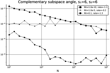
Figure 1. Complementary subspace angle $\beta$. $Nh$ and $\theta$ fixed, varying $N$.

In the second set of experiments, we kept the values of $N$ and $\theta$ fixed, while changing $h$. We chose again 3 different values $\theta=0.01,0.1,1$. The dependence of $\beta$ on $h$ (or $Nh$) in this case is shown in Figure 2. Notice that for small enough $Nh$ we indeed see that $\beta$ approaches a positive value which is proportional to ${1\over{N\theta}}$, i.e. the dominant role is played by the cluster separation. For increasing values of $Nh$, the actual cluster subspaces move further away from the limit spaces and therefore this regime is not covered by our theory. However, apparently also in this case $\beta$ remains small, but this must be due to other factors.

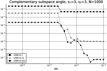
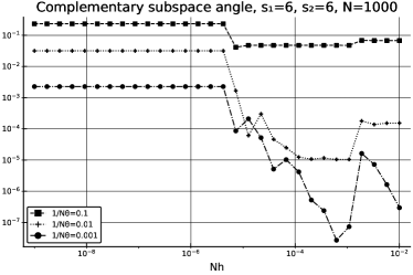
Figure 2. Complementary subspace angle $\beta$. $N,\theta$ fixed, varying $h$.

6.2. Spectra of multi-cluster Vandermonde matrices

We normalize the Vandermonde matrix and compute the spectra of the matrices ${1\over{\sqrt{N}}}\mathbf{V}_{N}(\mathcal{X})$. For each experiment we choose the values of $N$ and $h$ randomly from within a prescribed range. In the multi-cluster setting, we construct 2 nontrivial clusters of same size $h^{(1)}=h^{(2)}=h$, and add zero or more well-separated nodes (so if $s^{(1)}=2$, $s^{(2)}=3$ and $s=7$, there are 2 clusters of multiplicity 1). The values of $\sigma_{j}({1\over\sqrt{N}}\mathbf{V}_{N}(\mathcal{X}))$ for different $\mathcal{X}$ are plotted in Figure 3.

There is good agreement with Theorem 2.3 and Corollary 2.1. The proportionality constant is seen to be not too large. Furthermore, the minimal value of $Nh$ for which the bounds hold (corresponding to the constants $\Cr{single.cluster.Nh}$ and $\Cr{multi.cluster.N.h}$ in Theorems 2.3 and 2.2, respectively) is apparently reasonably high.

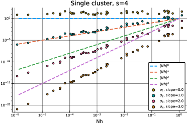
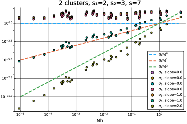
Figure 3. Singular values of ${1\over\sqrt{N}}\mathbf{V}_{N}$ as a function of $Nh$. (left) A single cluster with $s=4$. (right) 2 nontrivial clusters (and 4 overall), multiplicities = $2,1,3,1$. The slopes of the lines, computed by a linear fit, are written in the respective legend labels.

6.3. Least squares accuracy

Here we solve the least squares problem as in Theorem 2.4. In each experiment, we choose $N,h,\varepsilon$ uniformly at random within prescribed ranges. This in particular defines $\mathcal{X}$ and $\mathbf{V}_{N}(\mathcal{X})$. We then choose the entries of the vectors $\boldsymbol{\mathrm{a}}_{0}$ and $\boldsymbol{\mathrm{f}}$ to be uniformly randomly distributed in $\left[0,1\right]$. Then we put $\boldsymbol{\mathrm{b}}_{0}=\mathbf{V}_{N}(\mathcal{X})\boldsymbol{\mathrm{a}}_{0}$ and $\boldsymbol{\mathrm{b}}=\boldsymbol{\mathrm{b}}_{0}+\varepsilon\boldsymbol{\mathrm{f}}$. We then compute $\boldsymbol{\mathrm{a}}=\boldsymbol{\mathrm{a}}(\mathcal{X},\boldsymbol{\mathrm{b}})$ as in Definition 2.7. Finally, we set

$$\delta a_{\ell}:=\frac{|(\boldsymbol{\mathrm{a}}-\boldsymbol{\mathrm{a}}_{0})_{\ell}|}{\|\boldsymbol{\mathrm{b}}-\boldsymbol{\mathrm{b}}_{0}\|_{\infty}}.$$

We then repeat the experiment multiple times, and plot $\delta a_{\ell}$ for all $\ell=1,\dots,s$ as a function of $Nh$. The results are presented in Figure 4. There is a good agreement with the estimate (2.5) for each component.

Figure 4. Accuracy of least squares reconstruction. 2 nontrivial clusters (and 3 overall), multiplicities = $2,3,1$. The slopes of the lines, computed by a linear fit, are written in the respective legend labels.

Appendix A Divided differences

Recall Definition 3.1. The following properties can be found in e.g. [18], see also [8, Section 6.2].

Lemma A.1.

The functionals $[t_{1},\dots,t_{n}]$ satisfy the following.

1. $[t_{1},\dots,t_{n}]f$ is a symmetric function of $(t_{1},\dots,t_{n})$.

2. $[t_{1},\dots,t_{n}]f$ is a continuous function of $(t_{1},\dots,t_{n})$, i.e.

   $$\lim_{\left(t_{1},\dots,t_{n}\right)\to(u_{1},\dots,u_{n})}[t_{1},\dots,t_{n}]f=[u_{1},\dots,u_{n}]f.$$ (A.1)

3. The numbers $[t_{1},\dots,t_{n}]f$ can be computed by the recursive rule

   $$[t_{1},\dots,t_{n}]f=\begin{cases}f(t_{1})&n=1;\\ \frac{[t_{2},\dots,t_{n}]f-[t_{1},\dots,t_{n-1}]f}{t_{n}-t_{1}}&t_{1}\neq t_{n};\\ \lim_{\xi\to t_{n}}\bigl{\{}\frac{\textrm{d}}{\textrm{d}\xi}\left([\xi,t_{2},\dots,t_{n-1}]f\right)\bigr{\}}&t_{1}=t_{n}.\end{cases}$$ (A.2)

4. In particular, if all $\{t_{j}\}$’s are distinct, then

   $$[t_{1},\dots,t_{n}]f=\sum_{j=1}^{n}\frac{f(t_{j})}{\prod_{k\neq j}(t_{j}-t_{k})}.$$ (A.3)

5. (Mean value theorem) Let $t_{1},\dots,t_{n}\in\mathbb{R}$ and put $I:=\left[\min_{\ell}t_{\ell},\max_{\ell}t_{\ell}\right]$. Then

   $$[t_{1},\dots,t_{n}]f=\frac{f^{(n-1)}(\xi)}{(n-1)!},\quad\xi\in I.$$ (A.4)

6. From the above, in particular,

   $$[\underbrace{t,t,\dots,t}_{n\text{ times}}]f=\frac{f^{(n-1)}(t)}{(n-1)!}.$$ (A.5)

Appendix B Power sums

Lemma B.1.

For a positive integer $p$, the sum of the $p^{th}$ powers of the first $N+1$ non-negative integers is given by Faulhaber’s formula

$$\sum_{k=0}^{N}k^{p}=\frac{N^{p+1}}{p+1}+\frac{1}{2}N^{p}+\sum_{k=2}^{p}\frac{B_{k}}{k!}(p)_{k-1}N^{p-k+1}=\frac{N^{p+1}}{p+1}+\mathcal{O}(N^{p}),$$ (B.1)

where $B_{k}$ are the Bernoulli numbers, and $(p)_{k-1}$ is the falling factorial, $(p)_{k-1}=\dfrac{p!}{(p-k+1)!}$. We also have the following non-asymptotic bounds:

$$\frac{N^{p+1}}{p+1}=\int_{0}^{N}x^{p}\textrm{d}x\leq\sum_{k=0}^{N}k^{p}\leq N^{p+1}.$$ (B.2)

Appendix C Trigonometric cancellation

Lemma C.1.

For each $z\neq 1$ with $|z|=1$ and for each $m\in\mathbb{N}$ we have

$$\left|\sum_{k=0}^{N}k^{m}z^{k}\right|\leq\frac{2}{|1-z|}N^{m}.$$ (C.1)

Proof.

Let us notice that a “naive” upper bound

$$\left|\sum_{k=0}^{N}k^{m}z^{k}\right|\leq\sum_{k=0}^{N}k^{m}\sim N^{m+1}$$

is not sufficient for our purposes. To get the order of $N^{m}$ we have to take into account cancellations in the sum (C.1) as follows:

$$(1-z)\sum_{k=0}^{N}k^{m}z^{k}=-N^{m}z^{N+1}+\sum_{k=0}^{N}k^{m}z^{k}-\sum_{k=0}^{N-1}k^{m}z^{k+1}=-N^{m}z^{N+1}+\sum_{k=1}^{N}(k^{m}-(k-1)^{m})z^{k}.$$

Then by the triangle inequality

$$|1-z|\left|\sum_{k=0}^{N}k^{m}z^{k}\right|\leq N^{m}+\sum_{k=1}^{N}k^{m}-(k-1)^{m}=2N^{m}.$$

This completes the proof of Lemma C.1. ∎

References

- [1] A. Akinshin, D. Batenkov, and Y. Yomdin. Accuracy of spike-train Fourier reconstruction for colliding nodes. In 2015 International Conference on Sampling Theory and Applications (SampTA), pages 617–621, May 2015.
- [2] A. Akinshin, G. Goldman, and Y. Yomdin. Geometry of error amplification in solving Prony system with near-colliding nodes. arXiv:1701.04058 [math], Jan. 2017.
- [3] C. Aubel and H. Bölcskei. Vandermonde matrices with nodes in the unit disk and the large sieve. Applied and Computational Harmonic Analysis, Aug. 2017.
- [4] D. Batenkov. Stability and super-resolution of generalized spike recovery. Applied and Computational Harmonic Analysis, 45(2):299–323, Sept. 2018.
- [5] D. Batenkov, A. Bhandari, and T. Blu. Rethinking Super-resolution: The Bandwidth Selection Problem. In ICASSP 2019 - 2019 IEEE International Conference on Acoustics, Speech and Signal Processing (ICASSP), pages 5087–5091, May 2019.
- [6] D. Batenkov, L. Demanet, G. Goldman, and Y. Yomdin. Conditioning of Partial Nonuniform Fourier Matrices with Clustered Nodes. SIAM Journal on Matrix Analysis and Applications, 44(1):199–220, Jan. 2020.
- [7] D. Batenkov, G. Goldman, and Y. Yomdin. Super-resolution of near-colliding point sources. To appear in Information and Inference.
- [8] D. Batenkov and Y. Yomdin. Geometry and Singularities of the Prony mapping. Journal of Singularities, 10:1–25, 2014.
- [9] F. Bazán. Conditioning of rectangular Vandermonde matrices with nodes in the unit disk. SIAM Journal on Matrix Analysis and Applications, 21:679, 2000.
- [10] B. Beckermann. The condition number of real Vandermonde, Krylov and positive definite Hankel matrices. Numerische Mathematik, 85(4):553–577, 2000.
- [11] B. Beckermann and E. B. Saff. The sensitivity of least squares polynomial approximation. In Applications and Computation of Orthogonal Polynomials, pages 1–19. Springer, 1999.
- [12] B. Beckermann and A. Townsend. Bounds on the Singular Values of Matrices with Displacement Structure. SIAM Review, 61(2):319–344, Jan. 2019.
- [13] A. Ben-Israel and T. N. E. Greville. Generalized Inverses: Theory and Applications. Number 15 in CMS Books in Mathematics. Springer, New York, 2nd ed edition, 2003.
- [14] Å. Björck. Component-wise perturbation analysis and error bounds for linear least squares solutions. BIT, 31(2):237–244, 1991.
- [15] Å. Björck and G. H. Golub. Numerical methods for computing angles between linear subspaces. Mathematics of computation, 27(123):579–594, 1973.
- [16] M.-D. Choi. Tricks or treats with the Hilbert matrix. The American Mathematical Monthly, 90(5):301–312, 1983.
- [17] A. Cordova, W. Gautschi, and S. Ruscheweyh. Vandermonde matrices on the circle: Spectral properties and conditioning. Numerische Mathematik, 57(1):577–591, Dec. 1990.
- [18] C. deBoor. Divided differences. Surveys in Approximation Theory, 1:46–69, 2005. [Online article at] http://www.math.technion.ac.il/sat.
- [19] L. Demanet and N. Nguyen. The recoverability limit for superresolution via sparsity. 2014.
- [20] B. Diederichs. Well-Posedness of Sparse Frequency Estimation. arXiv:1905.08005 [math], May 2019.
- [21] D. Donoho. Superresolution via sparsity constraints. SIAM Journal on Mathematical Analysis, 23(5):1309–1331, 1992.
- [22] A. Eisinberg, P. Pugliese, and N. Salerno. Vandermonde matrices on integer nodes: The rectangular case. Numerische Mathematik, 87(4):663–674, Feb. 2001.
- [23] W. Gautschi. On inverses of Vandermonde and confluent Vandermonde matrices. Numerische Mathematik, 4(1):117–123, 1962.
- [24] W. Gautschi. On inverses of Vandermonde and confluent Vandermonde matrices. II. Numerische Mathematik, 5(1):425–430, 1963.
- [25] W. Gautschi. Norm estimates for inverses of Vandermonde matrices. Numerische Mathematik, 23(4):337–347, 1974.
- [26] W. Gautschi. On inverses of Vandermonde and confluent Vandermonde matrices III. Numerische Mathematik, 29(4):445–450, 1978.
- [27] N. J. Higham. A survey of componentwise perturbation theory in numerical linear algebra. In Proceedings of Symposia in Applied Mathematics, volume 48, pages 49–77, 1994.
- [28] J. A. Hogan and J. D. Lakey. Duration and Bandwidth Limiting: Prolate Functions, Sampling, and Applications. Springer Science & Business Media, Dec. 2011.
- [29] R. A. Horn and C. R. Johnson. Matrix Analysis. Cambridge University Press, Cambridge ; New York, 2nd ed edition, 2012.
- [30] A. V. Knyazev and M. E. Argentati. Principal angles between subspaces in an A-based scalar product: Algorithms and perturbation estimates. SIAM Journal on Scientific Computing, 23(6):2008–2040, 2002.
- [31] S. Kunis and D. Nagel. On the condition number of Vandermonde matrices with pairs of nearly-colliding nodes. arXiv:1812.08645 [math], Dec. 2018.
- [32] S. Kunis and D. Nagel. On the smallest singular value of multivariate Vandermonde matrices with clustered nodes. arXiv:1907.07119 [cs, math], July 2019.
- [33] H. B. Lee. Eigenvalues and eigenvectors of covariance matrices for signals closely spaced in frequency. IEEE Transactions on signal processing, 40(10):2518–2535, 1992.
- [34] W. Li and W. Liao. Stable super-resolution limit and smallest singular value of restricted Fourier matrices. arXiv:1709.03146 [cs, math], Sept. 2017.
- [35] W. Li, W. Liao, and A. Fannjiang. Super-resolution limit of the ESPRIT algorithm. IEEE Transactions on Information Theory, pages 1–1, 2020. Conference Name: IEEE Transactions on Information Theory.
- [36] C. A. Micchelli. Interpolation of scattered data: Distance matrices and conditionally positive definite functions. Constructive Approximation, 2(1):11–22, Dec. 1986.
- [37] A. Moitra. Super-resolution, Extremal Functions and the Condition Number of Vandermonde Matrices. In Proceedings of the Forty-Seventh Annual ACM on Symposium on Theory of Computing, STOC ’15, pages 821–830, New York, NY, USA, 2015. ACM.
- [38] V. Y. Pan. How Bad Are Vandermonde Matrices? SIAM Journal on Matrix Analysis and Applications, 37(2):676–694, Jan. 2016.
- [39] D. Slepian. A numerical method for determining the eigenvalues and eigenfunctions of analytic kernels. SIAM Journal on Numerical Analysis, 5(3):586–600, 1968.
- [40] D. Slepian. Prolate spheroidal wave functions, fourier analysis, and uncertainty – V: The discrete case. Bell System Technical Journal, The, 57(5):1371–1430, May 1978.
- [41] G. W. Stewart. Matrix perturbation theory. Academic Press, 1990.
- [42] P. Stoica and R. Moses. Spectral Analysis of Signals. Pearson/Prentice Hall, 2005.
- [43] J. Todd. The condition of the finite segments of the Hilbert matrix. Contributions to the solution of systems of linear equations and the determination of eigenvalues, 39:109–116, 1954.
- [44] T. E. Tuncer and B. Friedlander. Classical and Modern Direction-of-Arrival Estimation. Academic, London, 2009. OCLC: 299711034.
- [45] E. E. Tyrtyshnikov. How bad are Hankel matrices? Numerische Mathematik, 67(2):261–269, Mar. 1994.
- [46] A. J. Wathen and S. Zhu. On spectral distribution of kernel matrices related to radial basis functions. Numerical Algorithms, 70(4):709–726, Dec. 2015.
- [47] H. S. Wilf. Finite sections of some classical inequalities, volume 52. Springer Science & Business Media, 2012.
- [48] Z. Yang, J. Li, P. Stoica, and L. Xie. Chapter 11 - Sparse methods for direction-of-arrival estimation. In R. Chellappa and S. Theodoridis, editors, Academic Press Library in Signal Processing, Volume 7, pages 509–581. Academic Press, Jan. 2018.