Modelling our Galaxy

Abstract

Dynamical models will be key to exploitation of the incoming flood data for our Galaxy. Modelling techniques are reviewed with an emphasis on $f({\bf J})$ modelling.

1 Introduction

Since the second data release by the Gaia project in 2018 April we have been in possession of an enormous body of precision data for our very typical Galaxy. From satellites and ground-based telescopes we have astrometry and photometry (Gaia, Kepler, WISE, 2-Mass, SkyMapper, PanSTARRS) and spectra, largely taken from the ground, at sufficient resolution to infer chemical compositions (APOGEE, RAVE, LAMOST, Gaia-ESO). Data of increased precision for more stars will continue to arrive over the next $\sim$5 years. The task that lies before us is to use these data to understand how our Galaxy is structured, how it functions as a machine, and how it was assembled. Those tasks need to be addressed in roughly that order: it is pointless to speculate how the Galaxy was assembled until it is clear how it is structured, and not much more profitable to speculate about assembly until you understand how its dynamics causes its structure to evolve over cosmic time.

Dynamical models will be central to understanding how the Galaxy is structured. In the 1980s a significant step forward in our understanding of the Galaxy was taken when inversion of star counts (e.g. Bok, 1937) was replaced by forward modelling with star counts predicted by a sum of components – exponential disc, $r^{1/4}$ bulge, power-law stellar halo – derived from observations of external galaxies (Bahcall & Soneira, 1980; Caldwell & Ostriker, 1981). For many years, the de facto standard Galaxy model, the Besançon model (Robin et al., 2003), has been a development of this idea, in which the kinematics of stars are pasted onto a model derived from star counts. That is, at each location the distribution of stellar velocities is assumed to be bi- or tri-axial Gaussian with pre-determined principal axes. In reality the velocity distributions of a given component at different locations are coupled by dynamics.

The traditional approach to acknowledging this coupling is the use of Jeans’ moment equations, which relate the moments $\nu\left\langle v^{n}\right\rangle$ (with $\nu$ a component’s stellar number density) to the Galactic gravitational field $-\nabla\Phi$. There are many objections to this procedure. A basic one is that the Jeans’ equation for $\nu\left\langle v^{n}\right\rangle$ involves $\nu\left\langle v^{n+1}\right\rangle$ and an ansatz is required to close this hierarchy. Another problem is that velocity distributions are always significantly non-Gaussian and important information is contained in the deviations from Gaussianity. Consequently, the higher moments $\nu\left\langle v^{n}\right\rangle$ for $n>2$ are independent of the moments for $n=1$ (mean velocity) and $n=2$ (velocity dispersion), and adequate characterisation of the system requires values for the higher moments. It’s hard to recover them reliably from the Jeans equations (Magorrian & Binney, 1994).

2 Modelling methods

2.1 $f({\bf J})$ modelling

A promising approach to model building starts not with each component’s density $\nu({\bf x})$ but with its distribution function (DF) $f({\bf x},{\bf v})$. Once the DFs of every component is known, the system is completely specified in the sense that one can easily predict the outcome of any measurement; the set of DFs for a galaxy’s components is the galaxy’s DNA.

Models with specified DFs exploit Jeans’ theorem, which states that the DF of a steady-state system can be assumed to depend on $({\bf x},{\bf v})$ only through the constants of motion $I_{k}({\bf x},{\bf v})$. Specification of a stellar system by writing down a DF goes back to the origins of stellar dynamics (Eddington, 1916; Jeans, 1916) and it has played a major role in studies of globular clusters (Hénon, 1960; King, 1966). Until recently its application to galaxies was largely to spherical galaxies (Jaffe, 1983; Hernquist, 1990) and razor-thin discs (Kalnajs, 1977), despite brave efforts to apply it to S0 galaxies (Prendergast & Tomer, 1970; Rowley, 1988). All these early efforts were restricted to systems with single components, a serious restriction given the importance of dark matter and gradients in chemical composition and stellar age within galaxies: serious engagement with observational data requires multi-component models, which predict how colour varies through a system and relates this variation to velocity dispersions measured in different spectral lines.

In a steady-state system, energy $E$ is always a constant of motion, and all classical models make the DF a function of $E$. The key to multi-component modelling is to resist the temptation to put $E$ into the DF’s argument list. The reason is that the energy of an orbit is not a local quantity. For example, the simplest orbit is that on which the star sits at the galactic centre. If we add a shell of dark matter, the energy of this orbit will be depressed, but the orbit remains the same. When we write down the DF of the bulge or the stellar halo, we will want to specify the phase-space density of that component at this simplest orbit. But until the model is fully assembled and its potential has been determined, we don’t know the energy $E_{0}=\Phi(0)$ of this orbit. So we can’t specify $f(E,..)$ to begin model construction.

Much the best constants of motion to use as arguments of $f$ are the action integrals $J_{r}$, $J_{\phi}$ and $J_{z}$. The first of these quantifies the amplitude of oscillations in radius (eccentricity); in an axisymmetric system the second is simply the angular momentum around the symmetry axis; the last $J_{z}$ quantifies the amplitude of oscillations perpendicular to the equatorial plane. In addition to having simple physical interpretations, action integrals are adiabatic invariants: if the potential evolves over many dynamical times (perhaps because accretion of gas has built up a massive stellar disc), orbits evolve such that their actions remain the same. Consequently, $f({\bf J})$ is invariant under slow growth of a galaxy.

There should be as many independent actions as the system has spatial dimensions, and each action can be complemented by a canonically conjugate ‘angle’ variable $\theta_{i}$ such that the set $({\mathchoice{\hbox{{\gkvecten\char 18\relax}}}{\hbox{{\gkvecten\char 18\relax}}}{\hbox{{\gkvecseven\char 18\relax}}}{\hbox{{\gkvecseven\char 18\relax}}}},{\bf J})$ comprises a complete set of canonical coordinates for phase space. The equations of motion of these variables are trivial: clearly half the equations read ${\rm d}J_{i}/{\rm d}t=0$, while the other three equations read ${\rm d}\theta_{i}/{\rm d}t=\Omega_{i}({\bf J})$, a constant. Hence the angle variables increase linearly with time at the rate given by the frequencies $\Omega_{i}$. The way the system responds to perturbations is largely determined by how the frequencies $\Omega_{i}$ vary with actions, so these frequencies are of fundamental importance.

For decades the use of action integrals was impractical for lack of algorithms to translate between $({\bf x},{\bf v})$ and $({\mathchoice{\hbox{{\gkvecten\char 18\relax}}}{\hbox{{\gkvecten\char 18\relax}}}{\hbox{{\gkvecseven\char 18\relax}}}{\hbox{{\gkvecseven\char 18\relax}}}},{\bf J})$. Over the past decade the situation has improved hugely although it is still not entirely satisfactory. Excellent approximations to $\theta_{i}({\bf x},{\bf v})$ and $J_{i}({\bf x},{\bf v})$ for orbits in axisymmetric systems can be obtained from the Stäckel Fudge (Binney, 2012a), in which formulae strictly valid for Stäckel potentials are extended to general potentials. Vasiliev (2019) released very efficient code (AGAMA) to implementing the axisymmetric Fudge. Sanders & Binney (2015) extended the Stäckel Fudge to triaxial potentials with negligible figure rotation rates.

A radically different approach provides the inverse map: $[{\bf x}({\mathchoice{\hbox{{\gkvecten\char 18\relax}}}{\hbox{{\gkvecten\char 18\relax}}}{\hbox{{\gkvecseven\char 18\relax}}}{\hbox{{\gkvecseven\char 18\relax}}}},{\bf J}),{\bf v}({\mathchoice{\hbox{{\gkvecten\char 18\relax}}}{\hbox{{\gkvecten\char 18\relax}}}{\hbox{{\gkvecseven\char 18\relax}}}{\hbox{{\gkvecseven\char 18\relax}}}},{\bf J})]$. This is ‘torus mapping’. The surface specified by holding constant ${\bf J}$ and varying ` is a three-torus in six-dimensional phase space. Separation of the Hamilton-Jacobi equation for some potentials of high symmetry yields analytic expressions ${\bf x}({\mathchoice{\hbox{{\gkvecten\char 18\relax}}}{\hbox{{\gkvecten\char 18\relax}}}{\hbox{{\gkvecseven\char 18\relax}}}{\hbox{{\gkvecseven\char 18\relax}}}}^{\prime},{\bf J}^{\prime})$ for such tori, and the Torus Mapper (Binney & McMillan, 2016) computes the generating function $S({\mathchoice{\hbox{{\gkvecten\char 18\relax}}}{\hbox{{\gkvecten\char 18\relax}}}{\hbox{{\gkvecseven\char 18\relax}}}{\hbox{{\gkvecseven\char 18\relax}}}}^{\prime},{\bf J})$ that maps these tori into the orbital tori ${\bf x}({\mathchoice{\hbox{{\gkvecten\char 18\relax}}}{\hbox{{\gkvecten\char 18\relax}}}{\hbox{{\gkvecseven\char 18\relax}}}{\hbox{{\gkvecseven\char 18\relax}}}},{\bf J})$ of any specified axisymmetric potential.

It turns out that simple functional forms $f({\bf J})$ generate models that closely resemble classical models. Binney & McMillan (2011) defined a (‘quasi-isothermal’) DF that has exponential dependence on the actions that has been used in several studies to represent exponential discs (e.g. Binney, 2012b; Bovy & Rix, 2013; Piffl et al., 2014). Posti et al. (2015) gave a form that self-consistently generates double-power-law components including the NFW and Hernquist spheres. Pascale et al. (2018, 2019) gave a form that self-consistently generates objects that resemble dwarf spheroidal galaxies and globular clusters.

Using these pre-defined DFs a model of a composite system like our Galaxy is quickly generated: a DF $f_{k}({\bf J})$ is specified for the dark halo and each stellar component. The mass $M_{k}$ of each component is specified by the normalisation chosen or $f_{k}$ because $M_{k}=(2\pi)^{3}\int{\rm d}^{3}{\bf J}\,f_{k}$. Then a rough guess $\Phi_{0}$ is made of the galaxy’s total potential and this guess is used to evaluate the density $\rho_{k}({\bf x})$ of each component on a grid of locations ${\bf x}$. From these densities and Poisson’s equation one recovers a new estimate of the total potential $\Phi_{1}$, which is used to re-evaluate the densities, so an improved potential $\Phi_{2}$ can be recovered. This sequence of densities and potentials reliably converges after $\sim 5$ iterations. Then the model is complete and ready to predict any observable.

2.2 Schwarzschild modelling

An orbital torus $[{\bf x}({\mathchoice{\hbox{{\gkvecten\char 18\relax}}}{\hbox{{\gkvecten\char 18\relax}}}{\hbox{{\gkvecseven\char 18\relax}}}{\hbox{{\gkvecseven\char 18\relax}}}},{\bf J}),{\bf v}({\mathchoice{\hbox{{\gkvecten\char 18\relax}}}{\hbox{{\gkvecten\char 18\relax}}}{\hbox{{\gkvecseven\char 18\relax}}}{\hbox{{\gkvecseven\char 18\relax}}}},{\bf J})]$ is a powerful extension of a numerically integrated orbit $[{\bf x}(t),{\bf v}(t)]$. Schwarzschild (1979) introduced the idea of assembling galaxies by weighting orbits computed in a trial potential, and this idea has been used extensively to model elliptical and spheroidal galaxies (e.g. van den Bosch et al., 2008; Zhu et al., 2018). Replacing orbits (time series) with orbital tori has many advantages:

• One can quickly find the velocity ${\bf v}$ at which a torus will visit a given location ${\bf x}_{0}$, while a finite time series is unlikely to include ${\bf x}_{0}$;

• It’s much easier to ensure that a torus library, rather than an orbit library, samples phase space systematically and with pre-defined density;

• A torus is typically specified by less than 100 numbers, whereas an orbit requires tens of thousands of numbers for its specification;

• An infinity of new tori can be obtained by interpolating between the tori of a grid;

• Angle-action variables are the language of Hamiltonian perturbation theory, so a torus-based model can be used to determine how a galaxy responds to perturbations (Monari et al., 2016; Binney, 2018).

I believe that in Schwarzschild modelling tori provide superior replacements for any quasi-periodic orbit that is a member of the principal families identified by Schwarzschild (1979) and de Zeeuw (1985). As I’ll explain below, orbital tori can also replace resonantly trapped orbits. The extent to which they can replace chaotic orbits is still an open question.

2.3 N-body modelling

N-body models are enormously flexible and pretty easy to make. Over the last half century N-body codes have grown enormously in speed and precision, to the point that a good basic model can be run on a quality laptop and it’s practical to produce a suite simulations with tens of millions of particles on a small cluster.

A key issue is the level of Poisson (shot) noise. The Galaxy’s dark halo contains $\sim 10^{12}{\rm\,M_{\odot}}$ and the Poisson noise to which it gives rise heats a realistically thin disc at an unacceptable rate if it is represented by fewer than a few million particles (e.g. Aumer et al., 2016). Our observational data constrain the disc within $\mathrel{\hbox to0.0pt{\lower 3.0pt\hbox{$\mathchar 536\relax$}\hss}\raise 2.0pt\hbox{$\mathchar 316\relax$}}1\,{\rm kpc}$ from the Sun, a region that contains only $\sim 0.24\%$ of the disc’s stars. Hence with $10^{6}$ particles representing the disc, comparisons with data will be based on $\sim 2400$ phase-space points. This number is too small given that one needs to examine changes with $|z|$ and split the disc into components by age and chemistry: stars young and old, metal-poor and metal-rich, low or high in $\alpha$-abundance, etc.

Another key issue with N-body models is initial conditions: they specify the equilibrium model that you get after integrating for a few dynamical times. If the initial conditions lie far from equilibrium, as in a simulation of cosmological clustering, adjusting the initial conditions is not a viable way to steer the model towards conformity with observational data. Hence cosmological simulations don’t offer a promising way to construct a model of our Galaxy as we find it now. Rather they are a tool with which to explore, in a general way, how galaxies like ours might have formed.

An N-body model is specified by $\mathrel{\hbox to0.0pt{\lower 3.0pt\hbox{$\mathchar 536\relax$}\hss}\raise 2.0pt\hbox{$\mathchar 318\relax$}}10^{8}$ numbers, the phase-space coordinates of its particles. With every timestep, all these numbers change while an equilibrium model does not. Hence the numbers are highly redundant and the model is needlessly cumbersome. We might be able to gain insight into the essential structure of an N-body model by fitting its particle distribution to DFs $f({\bf J})$ for a disc, a bulge, and stellar and dark halos. Such a fit would simultaneously reduce the model to a few dozen numbers and give physical insight into its structure.

Perhaps the most promising way to initialise an N-body model of our Galaxy is to draw initial conditions from an equilibrium model constructed by the $f({\bf J})$ technique – the AGAMA package provides a fast routine for furnishing initial conditions. N-body models initialised in this way provide the best available tool with which to investigate the collective dynamics of discs: since the unperturbed model is accurately in equilibrium, time-dependent features can be reliably ascribed to whatever perturbation one has applied. Moreover, analytic understanding of why the model responds as it does is facilitated by the knowledge of the equilibrium DF as a function of actions. The prospects for gaining an adequate understanding of spiral structure and warps by this route seem bright.

2.4 Made-to-measure modelling

By far the best current model of the Galactic bulge/bar is that constructed by Wegg et al. (2015) by the made-to-measure (M2M) technique. This may be considered a hybrid of the N-body and Scharzschild techniques: one starts with an N-body model and progressively modifies the weights with which orbits contribute to the overall density and observables so as to optimise the fit the model provides to observations. Effectively, the N-body model provides the orbit library, while a ‘force for change’ (Syer & Tremaine, 1996) replaces linear or quadratic programming as the algorithm for choosing orbit weights. The technique can model any type of galaxy and is relatively easy to implement. Its main drawback is that, like any N-body model, it is specified by $\sim 10^{8}$ numbers that individually lack significance.

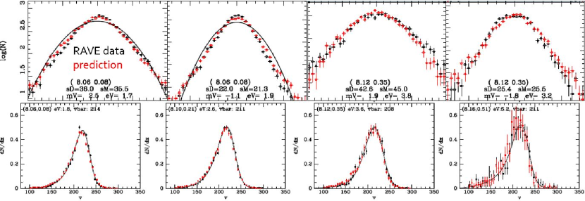
Figure 1: Velocity distributions of red dwarfs from the RAVE survey (black points) compared to predictions (red) of DFs fitted to data from the GCS survey. The top row shows histograms for $V_{R}$ and $V_{z}$ at $\sim R_{0}$ near the plane (left two panels) and at $|z|\sim 0.35\,{\rm kpc}$. The lower row shows $V_{\phi}$ distributions at distances from the plane that increase from left to right with the furthest bin centre at $0.51\,{\rm kpc}$.

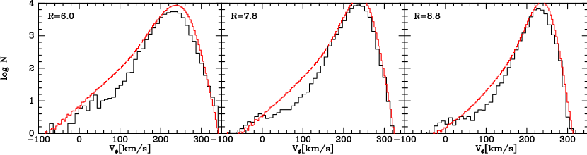
Figure 2: Distributions of $V_{\phi}$ a locations near the plane and radii $R=6$, $7.6$ and $8.8\,{\rm kpc}$ from RVS data (black) and the predictions of a fully self-consistent model for bin centres (red). The peaks of the histograms are determined by the circular-speed curve of the recovered potential shown in Fig. 3.

Figure 3: Circular speed curve of a self-consistent Galaxy model fitted to Gaia DR2 RVS data. The broken curves show the contributions from the dark halo (long dashed) disc (short dashed) and the bulge (dotted). The yellow shaded region shows the probable zone of $V_{c}$ inferred from Cepheids by Mróz et al. (2019)

3 Examples of $f({\bf J})$ modelling

3.1 Our Galaxy

Binney (2012b) fitted quasi-isothermal DFs for the thin and thick discs to data from the Geneva-Copenhagen survey (Nordström et al., 2004; Holmberg et al., 2009). In figures like Fig. 1, Binney et al. (2014) compared the predictions of these DFs to the newly available data from the RAVE survey (Zwitter et al., 2008). The agreement between data (black) and prediction (red) is spectacular. The parabolas in the two panels at top left show Gaussian distributions and one sees that the model reproduces the non-Gaussianity of the data, just as it reproduces the skewness of the $V_{\phi}$ distributions shown in the lower panels.

In work prior to 2015 the dark halo was specified by a density distribution rather than a DF. Piffl et al. (2015) opened a new chapter by specifying the dark halo through its DF, and Binney & Piffl (2015) fitted such a model to data from several sources, including RAVE and terminal velocities from HI and CO observations. The heterogeneous nature of their data and limitations of the software available to them made the fitting process tortuous and costly. Gaia DR2 data now extend over a sufficiently large radial range that one can dispense with terminal velocities and determine the structure of the dark halo from stars alone. Fig. 2 shows an example: the black histograms are velocity distributions from the RVS sample in DR2 binned in real space using the distances of Schönrich et al. (2019), while red curves show a model’s predictions for the centre of the bin. The location of the peak in $V_{\phi}$ is determined by the circular-speed curve of the derived potential. Fig. 3 shows that curve in black together with the contributions to it from the dark halo (long-dashed), disc (short-dashed) and bulge (dotted).

Figure 4: Star counts (upper row) and velocity dispersions (lower row) in the Fornax dSph compared to predictions of three models. Left column: a model in which the dark halo has a DF that in isolation generates an NFW profile; middle and right columns: models in which the dark halo’s DF generates a core.

3.2 The Fornax dwarf spheroidal galaxy

Since stars currently contribute little to the gravitational potentials of dwarf spheroidals, it has often been argued that these systems have pristine dark halos in which we can test the prediction of dark-matter-only cosmological simulations that such halos should have cuspy cores. Pascale et al. (2018) built $f({\bf J})$ models of the Fornax dSph in which the dark halo was specified by a DF that either did, or did not, generate a central cusp. The upper row of Fig. 4 shows that excellent fits to the star counts could be obtained with both types of halo DF, but the lower row shows that the data for velocity dispersion unambiguously favour a DF that does not generate a cusp.

Figure 5: A surface of section for an axisymmetric Galactic potential in a region of resonant trapping. Consequents of numerically integrated orbits are shown in blue, with cross sections of tori computed with the Torus Mapper in magenta. The green curves show the untrapped tori used by the Torus Mapper. (From Binney, 2016)

4 Resonant trapping

Even in an axisymmetric potential, it’s not possible to assign values of $J_{r}$, $J_{z}$ and $J_{\phi}$ to every orbit. Some orbits become ‘trapped’ by a resonance. Fortunately, the Torus Mapper provides tools that yield astonishingly accurate analytic representations of the tori of trapped orbits such as those shown in Fig. 5. Binney (2018) showed that the same tools can be used to obtain analytic representations of the orbital tori of rotating barred potentials. Trapped orbits constitute a large topic that I haven’t space to explore. From the perspective of $f({\bf J})$ modelling, they are a complication because each family of trapped orbits has it’s own angle-action coordinates and requires its own DF $f({\bf J})$. Trapped orbits permit kinematics that can differ qualitatively from what would be possible in the absence of trapping, such as circulation in the $(R,z)$ plane (Binney & McMillan, 2016). The discovery that at $|V_{z}|\sim 80\,{\rm km\,s^{-1}}$ more (thick disc) stars are passing up/down through the plane than down/up would provide a valuable constraint on $\Phi$ by locating the prominent $\Omega_{r}=\Omega_{z}$ resonance.

References

- Aumer et al. (2016) Aumer M., Binney J., Schönrich R., 2016, MNRAS, 459, 3326
- Bahcall & Soneira (1980) Bahcall J. N., Soneira R. M., 1980, ApJS, 44, 73
- Binney (2012a) Binney J., 2012a, MNRAS, 426, 1324
- Binney (2012b) Binney J., 2012b, MNRAS, 426, 1328
- Binney (2016) Binney J., 2016, MNRAS, 462, 2792
- Binney (2018) Binney J., 2018, MNRAS, 474, 2706
- Binney et al. (2014) Binney J., Burnett B., Kordopatis G., Steinmetz M., et al. 2014, MNRAS, 439, 1231
- Binney & McMillan (2011) Binney J., McMillan P., 2011, MNRAS, 413, 1889
- Binney & McMillan (2016) Binney J., McMillan P. J., 2016, MNRAS, 456, 1982
- Binney & Piffl (2015) Binney J., Piffl T., 2015, MNRAS, 454, 3653
- Bok (1937) Bok B. J., 1937, The Distribution of the Stars in Space
- Bovy & Rix (2013) Bovy J., Rix H.-W., 2013, ApJ, 779, 115
- Caldwell & Ostriker (1981) Caldwell J. A. R., Ostriker J. P., 1981, ApJ, 251, 61
- de Zeeuw (1985) de Zeeuw T., 1985, MNRAS, 216, 273
- Eddington (1916) Eddington A. S., 1916, MNRAS, 76, 572
- Hénon (1960) Hénon M., 1960, Annales d’Astrophysique, 23, 474
- Hernquist (1990) Hernquist L., 1990, ApJ, 356, 359
- Holmberg et al. (2009) Holmberg J., Nordström B., Andersen J., 2009, A&A, 501, 941
- Jaffe (1983) Jaffe W., 1983, MNRAS, 202, 995
- Jeans (1916) Jeans J. H., 1916, MNRAS, 76, 567
- Kalnajs (1977) Kalnajs A. J., 1977, ApJ, 212, 637
- King (1966) King I. R., 1966, AJ, 71, 64
- Magorrian & Binney (1994) Magorrian J., Binney J., 1994, MNRAS, 271, 949
- Monari et al. (2016) Monari G., Famaey B., Siebert A., 2016, MNRAS, 457, 2569
- Mróz et al. (2019) Mróz P., Udalski A., Skowron D. M., Skowron J., Soszyński I., Pietrukowicz P., Szymański M. K., Poleski R., Kozłowski S., Ulaczyk K., 2019, ApJL, 870, L10
- Nordström et al. (2004) Nordström B., Mayor M., Andersen J., Holmberg J., Pont F., Jørgensen B. R., Olsen E. H., Udry S., Mowlavi N., 2004, A&A, 418, 989
- Pascale et al. (2019) Pascale R., Binney J., Nipoti C., Posti L., 2019, MNRAS, 488, 2423
- Pascale et al. (2018) Pascale R., Posti L., Nipoti C., Binney J., 2018, MNRAS, 480, 927
- Piffl et al. (2014) Piffl T., Binney J., McMillan P. J., Bienaymé O., Bland-Hawthorn J., Freeman K., Gibson B., Gilmore G., Grebel E. K., Helmi A., Kordopatis G., Navarro J. F., Parker Q., Reid W. A., Seabroke G., Siebert A., Steinmetz M., Wyse R. F. G., 2014, MNRAS, 445, 3133
- Piffl et al. (2015) Piffl T., Penoyre Z., Binney J., 2015, MNRAS, 451, 639
- Posti et al. (2015) Posti L., Binney J., Nipoti C., Ciotti L., 2015, MNRAS, 447, 3060
- Prendergast & Tomer (1970) Prendergast K. H., Tomer E., 1970, AJ, 75, 674
- Robin et al. (2003) Robin A. C., Reylé C., Derrière S., Picaud S., 2003, A&A, 409, 523
- Rowley (1988) Rowley G., 1988, ApJ, 331, 124
- Sanders & Binney (2015) Sanders J. L., Binney J., 2015, MNRAS, 447, 2479
- Schönrich et al. (2019) Schönrich R., McMillan P., Eyer L., 2019, MNRAS, 487, 3568
- Schwarzschild (1979) Schwarzschild M., 1979, ApJ, 232, 236
- Syer & Tremaine (1996) Syer D., Tremaine S., 1996, MNRAS, 282, 223
- van den Bosch et al. (2008) van den Bosch R. C. E., van de Ven G., Verolme E. K., Cappellari M., de Zeeuw P. T., 2008, MNRAS, 385, 647
- Vasiliev (2019) Vasiliev E., 2019, MNRAS, 482, 1525
- Wegg et al. (2015) Wegg C., Gerhard O., Portail M., 2015, MNRAS, 450, 4050
- Zhu et al. (2018) Zhu L., van de Ven G., Méndez-Abreu J., Obreja A., 2018, MNRAS, 479, 945
- Zwitter et al. (2008) Zwitter T., Siebert A., Munari U., Freeman K. C., Siviero A., et al. 2008, AJ, 136, 421