Positive quantum Lyapunov exponents in experimental systems with a regular classical limit
Abstract
Quantum chaos refers to signatures of classical chaos found in the quantum domain. Recently, it has become common to equate the exponential behavior of out-of-time order correlators (OTOCs) with quantum chaos. The quantum-classical correspondence between the OTOC exponential growth and chaos in the classical limit has indeed been corroborated theoretically for some systems and there are several projects to do the same experimentally. The Dicke model, in particular, which has a regular and a chaotic regime, is currently under intense investigation by experiments with trapped ions. We show, however, that for experimentally accessible parameters, OTOCs can grow exponentially also when the Dicke model is in the regular regime. The same holds for the Lipkin-Meshkov-Glick model, which is integrable and also experimentally realizable. The exponential behavior in these cases are due to unstable stationary points, not to chaos.
Classical chaos in Hamiltonian systems is typically defined by means of the sensitive dependence on initial conditions, which leads to positive Lyapunov exponents (LEs) Ott (2002). But this alone is not a complete definition of chaos. Consider, for example, the simple pendulum. Its upright position corresponds to a stationary point that is unstable. It has a positive LE, as any genuine chaotic system, although it is completely integrable. The pendulum does not exhibit chaotic behaviors, such as non-periodicity and mixing Gaspard (1998). Its unstable point and the phase-space orbits emanating from it have measure zero with respect to the rest of the phase space. In this work, we investigate what happens to such unstable points in the quantum domain.
It was argued in Rozenbaum et al. that quantum mechanics can bring chaos to classical systems that are non-chaotic. This idea was inspired by Ref. Bunimovich (2019), where a standard non-chaotic classical billiard became chaotic when the point particle was substituted by a finite-size hard sphere. By making a parallel between the semiclassical dynamics of a quantum wave packet and the motion of a finite-size classical particle, it was shown in Rozenbaum et al. that quantum chaos can emerge in regular classical billiards. Quantum chaos in this case refers to the exponentially fast growth of the out-of-time ordered correlator (OTOC) at short times.
The OTOC quantifies the degree of noncommutativity in time between two operators. It was introduced in the context of superconductivity Lar to measure the instability of the trajectories of electrons scattered by impurities. Recently, the OTOC became a key quantity in definitions of many-body quantum chaos Kitaev ; Maldacena and Stanford (2016); Maldacena et al. (2016); Roberts and Stanford (2015); Fan et al. (2017); Luitz and Bar Lev (2017); Torres-Herrera et al. (2018); Borgonovi et al. (2019); Yan et al. (2019), analysis of the quantum-classical correspondence of chaotic systems Rozenbaum et al. (2017, 2019); Hashimoto et al. (2017); Chávez-Carlos et al. (2019); García-Mata et al. (2018); Jalabert et al. (2018); Fortes et al. (2019); Rammensee et al. (2018); Lakshminarayan (2019), and studies of the scrambling of quantum information Gärttner et al. (2018); Lewis-Swan et al. (2019) and quantum phase transitions Shen et al. (2017); Wang and Pérez-Bernal (2019a). The OTOC has been measured experimentally with ion traps Gärttner et al. (2017) and nuclear magnetic resonance platforms Li et al. (2017); Wei et al. (2018); Niknam et al. .
Depending on how the OTOC is computed, it may be called microcanonical OTOC (MOTOC) Hashimoto et al. (2017), fidelity OTOC (FOTOC) Lewis-Swan et al. (2019), thermal OTOC Maldacena et al. (2016), and OTOC for specific initial states Rozenbaum et al. (2017, ). The exponential growth rate of the latter, of the MOTOC Chávez-Carlos et al. (2019), and of the FOTOC Lewis-Swan et al. (2019) was shown to be related with the classical LE of chaotic systems. This has justified referring to the OTOCs exponential growth rates as quantum LEs and associating their exponential behavior with the notion of quantum chaos.
However, based on a semiclassical quantization approach, it was recently shown that, in general, the OTOC can grow exponentially fast also in one-degree-of-freedom quantum systems that are not globally chaotic, but are critical Hummel et al. (2019). Here, we show that this happens also for the Dicke model, which has two degrees of freedom and is used to describe strongly interacting light-matter systems Dicke (1954); Garraway (2011); Kirton et al. (2019). The Dicke model presents chaotic and regular regimes and is of great experimental relevance. It has been realized experimentally with cold atoms Baumann et al. (2010, 2011); Ritsch et al. (2013); Klinder et al. (2015), by means of cavity Raman transitions Baden et al. (2014); Zhang et al. (2018), and with ion traps Safavi-Naini et al. (2018). We study the FOTOC, because this quantity is directly measured by trapped ion experiments, and consider parameters and initial states used in these experiments.
The Dicke model has unstable points that give rise to positive LEs in the regular regime. These points and the orbits emanating from them have measure zero foo (a). In the quantum domain, on the other hand, we find that the FOTOC grows exponentially not only for initial states centered at the classically unstable point, but also for generic states centered at the surrounding points with zero classical LEs. Quantum mechanics therefore generates instability in a region where the classical dynamics is stable. Following the current terminology, we then refer to these regions as “quantum chaotic”, although one may ponder whether, similarly to the above discussion about classical chaos, additional conditions, on top of the exponential growth of the OTOCs, are needed for defining quantum chaos.
The OTOC grows exponentially also at the critical point of the Lipkin-Meshkov-Glick (LMG) model Pappalardi et al. (2018). This is a one-degree of freedom classically integrable system introduced in nuclear physics Lipkin et al. (1965a); *Lipkin1965b; *Lipkin1965c and realized experimentally with cold atoms Gross et al. (2010); Zibold et al. (2010) and nuclear magnetic resonance platforms Araujo-Ferreira et al. (2013). By studying the FOTOC, we show that the exponential behavior persists in the vicinity of this critical point as well.
The unstable points of the LMG and Dicke models. In a classical Hamiltonian system with real first-order differential equations , where are the generalized coordinates and momenta, a point is stationary when . This point is unstable when at least one of the positive-negative pairs of eigenvalues of the Jacobian matrix of evaluated at has a nonzero real part. The LE of this point equals the maximum of these real part values [see the Supplemental Material (SM) in SM for more details]. Both the LMG and the Dicke model in the classical limit present stationary points with positive LEs.
The LMG model Lipkin et al. (1965a); *Lipkin1965b; *Lipkin1965c describes the collective motion of a set of two-level systems mutually interacting. Its quantum Hamiltonian is given by
| (1) |
where , is the energy difference of the two-level systems, is the coupling strength, are the collective pseudospin operators given by the sum of Pauli matrices for each two-level system , and gives the size of the system, with being the eigenvalue of the total spin operator . This model has been employed, for example, in studies of ground state quantum phase transitions (QPTs) and excited state quantum phase transitions (ESQPTs) Caprio et al. (2008); Cejnar et al. (2010); Santos and Pérez-Bernal (2015); Santos et al. (2016), entanglement Vidal (2004); Dusuel and Vidal (2004), and quantum speed limit Wang and Pérez-Bernal (2019b).
The classical LMG Hamiltonian is obtained by taking the expectation value of on Bloch coherent states , where is the state with the lowest pseudospin projection and is the raising operator. Defining in terms of the canonical variables as and neglecting terms, the classical LMG Hamiltonian reads
| (2) |
Hamiltonian (2) is regular, but its stationary point is unstable and presents a positive LE given by
| (3) |
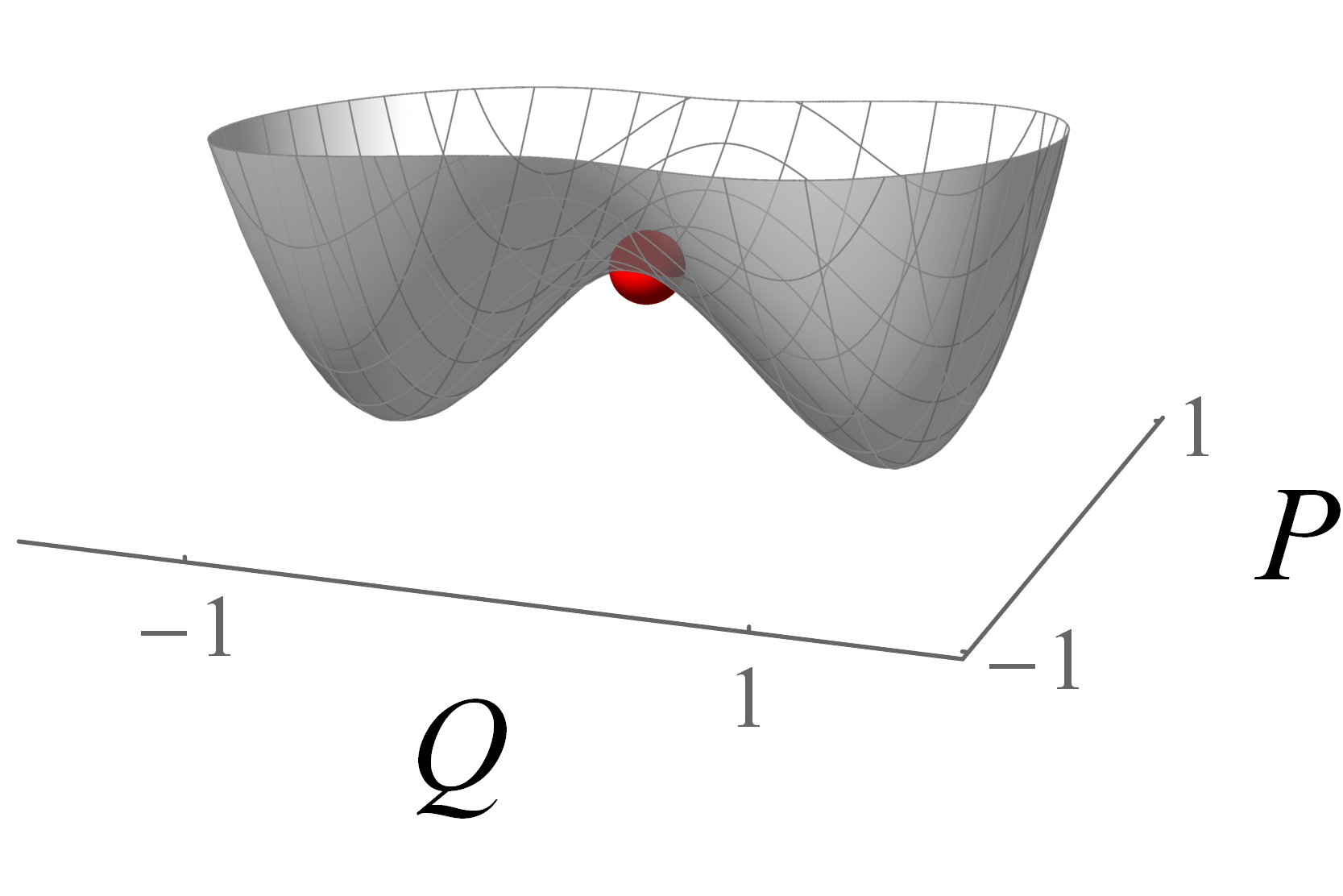
when (see Pappalardi et al. (2018) and SM SM ). Figures 1(a) and 1(b) show the energy surface of the classical LMG model for and two values of . When , is a minimum, while for , becomes a saddle point and is therefore unstable.
In the quantum domain, this saddle point is associated with an ESQPT. A main signature of ESQPTs is the divergence of the density of states at an energy denoted by . In the mean-field approximation, it has been shown that this energy coincides with the energy of the classical system at the saddle point Cejnar et al. (2006); Caprio et al. (2008), that is, for the LMG model, .
 |
 |
| (a) | (b) |
 |
|
| (c) | |
The Dicke model is a collection of two-level atoms of level spacing coupled to a quantized radiation field of frequency . The Hamiltonian is given by
| (4) |
where and , with being the annihilation (creation) operator, and is the atom-field interaction strength. As in the LMG model, in the symmetric atomic subspace, .
The Dicke model was first used to explain the collective phenomenon of superradiance Dicke (1954); Hepp and Lieb (1973); *Wang1973; *Carmichael1973. It is now used in studies of QPTs and ESQPTs Hepp and Lieb (1973); *Wang1973; *Carmichael1973; Castaños et al. (2005); Pérez-Fernández et al. (2011a); Brandes (2013); Bastarrachea-Magnani et al. (2014a); Larson and Irish (2017), quantum chaos Lewenkopf et al. (1991); Emary and Brandes (2003a); *Emary2003; Bastarrachea-Magnani et al. (2014b); *Bastarrachea2015; *Bastarrachea2016PRE; Chávez-Carlos et al. (2016), monodromy Babelon et al. (2009); Kloc et al. (2017a), entanglement creation Schneider and Milburn (2002); *Lambert2004; *Kloc2017, nonequilibrium dynamics Pérez-Fernández et al. (2011b); Altland and Haake (2012); Lerma-Hernández et al. (2018, 2019); Kloc et al. (2018), OTOC behavior Alavirad and Lavasani (2019); Lewis-Swan et al. (2019), and quantum batteries Andolina et al. (2019).
The classical Dicke Hamiltonian Ribeiro et al. (2006); Bakemeier et al. (2013); Chávez-Carlos et al. (2016) is obtained by taking the expectation value of between the product of Bloch coherent states and Glauber coherent states where , and is the photon vacuum. In terms of the canonical variables for the pseudospin and for the field SM , it reads
| (5) |
The stationary point of the Dicke model is . The LE associated with it can be calculated in terms of , , and , as (see SM SM )
| (6) |
When , this equation gives a positive value for the LE and the stationary point is unstable. When , Eq. (6) has pure imaginary values and the LE is zero. The critical point marks the ground state QPT of the Dicke model. For , the system is in the superradiant phase, and for , it is in the normal phase. The unstable point is therefore in the superradiant phase.
Energy surfaces similar to those in Figs. 1(a) and 1(b) can also be drawn for the Dicke model, but in higher dimension. The saddle point of this model is also associated with an ESQPT Bastarrachea-Magnani et al. (2014a), which happens at . We stress that, contrary to common belief, the ESQPT in the Dicke model is not directly related with the transition to classical chaos Chávez-Carlos et al. (2016); Relaño et al. (2016).
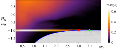
In Fig. 1 (c), we show the largest LEs of the Dicke model as functions of the classical excitation energy and of the atomic frequency , for and . Employing frequency units of kHz/, these values coincide with those used in the experiment with ion traps Lewis-Swan et al. (2019); Safavi-Naini et al. (2018). The blue line in the figure depicts the ground state energy and the gray area under it is forbidden. The color gradient indicates the presence or absence of chaos: black represents regular regions and light areas have large LEs. The bright horizontal line at the ESQPT, , indicates very large LEs and reflects the instability.
According to Eq. (6), the maximum LE is obtained for , which is approximately the value used in Lewis-Swan et al. (2019). As one sees in Fig. 1 (c), this classical instability is immersed in a chaotic region of the phase space with positive LEs, so we show some results for it only in the SM SM . Here, our main focus is on the unstable point at , which is marked in the figure with a red square. The phase-space region surrounding this unstable point is regular, with zero LEs everywhere, except for the phase-space orbits emanating from it Chávez-Carlos et al. (2016); foo (b). This is the unstable point that we use in our studies in Fig. 3. But before showing those results, let us describe how the quantum and classical evolutions are carried out and compared.
Quantum-classical correspondence.– The OTOC measures the degree of non-commutativity in time between operators and , . It is known as FOTOC when , where is a Hermitian operator and is a small perturbation, and is the projection operator onto the initial state. In the perturbative limit, , the dynamics of the FOTOC agrees with that of the variance of (see Lewis-Swan et al. (2019) and SM SM ),
| (7) |
so we refer to this variance as FOTOC and denote its exponential growth rate by . In what follows, we refer to as the quantum LE.
The FOTOC enables a direct visualization of the quantum evolution in terms of the dynamics in phase space. It measures the spread of the size of the wave packet and can thus be compared with the variance of the canonical variables in phase space.
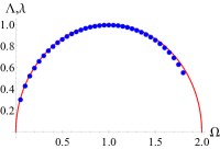
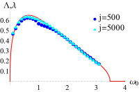
To compute the FOTOC, we consider initial Bloch coherent states for the LMG model, and initial products of Bloch and Glauber coherent states for the Dicke model. In Fig. 2, we compare the quantum LE obtained for the FOTOC with the classical LE for the LMG (a) and the Dicke (b) model at an unstable point. For the LMG model, the quantum evolution is done exactly. Since the wave packet spreads in both directions in phase space, we analyze the growth of . The agreement between from Eq. (3) and is perfect.
 |
 |
| (a) LMG model | (b) Dicke model |
A great advantage of the FOTOC is that it can be computed with semiclassical phase-space methods, such as the truncated Wigner approximation (TWA) Steel and Collett (1998, 1998); Polkovnikov (2010); Schachenmayer et al. (2015); Schmitt et al. (2019), which makes accessible system sizes that are not achievable with exact diagonalization. This is particularly useful for the Dicke model, which is nonintegrable and where the number of bosons in the field is not limited.
The basic idea of the TWA Polkovnikov (2010) is to compute the dynamics using the classical equations of motion, but averaging the observable over a large sample of initial conditions and replacing the classical probability distribution with the Wigner function Wigner (1932) and the classical observable with the Weyl symbol of the corresponding quantum operator Weyl (1927). The random sampling reproduces the quantum fluctuations of a quantum initial state.
The FOTOC that we study for the Dicke model is . Employing an efficient basis for the convergence of the eigenstates Bastarrachea-Magnani and Hirsch (2014), we evaluate the exact quantum evolution for , where the truncated Hilbert space has 24 453 converged eigenstates. We verify that for this size, which is already large for exact diagonalization, the exact quantum evolution and the evolution done with the TWA agree extremely well from up to times beyond the exponential growth of the FOTOC (see SM SM ). This assures us that we can use the TWA to calculate for larger ’s. For coherent states, the initial Wigner functions are positive and approximately given by normal distributions. Our sampling is done by means of a Monte Carlo method Schachenmayer et al. (2015) over random points (see details in SM SM ). As one increases from to , the agreement between from Eq. (6) and the quantum LE improves, as seen in Fig. 2 (b).
For our set of parameters, the Dicke model can be separated in fast and slow modes at the ESQPT energy Bastarrachea-Magnani et al. (2017). For the slow mode, an ESQPT as in an effective one-degree-of-freedom Hamiltonian emerges. This confirms the conjecture in Hummel et al. (2019) that their results might apply also to models with more than one degree of freedom.
Quantum activation of the instability. The results above make evident that, despite the regularity of the systems, both classical and quantum LEs coincide and are positive at the unstable points. We now investigate what happens at the vicinity of the unstable point of the LMG model with and of the Dicke model with . Classically, the LEs in these surrounding regions, in orbits not asymptotically going to or coming from the unstable point, are zero. To analyze what happens in the quantum domain, we study the behavior of the FOTOC as one moves away from the unstable point.
 |
 |
| (a) | (b) |
 |
 |
| (c) | (d) |
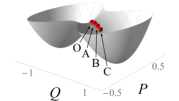
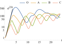
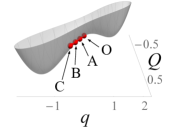
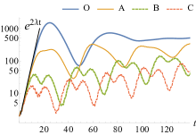
The unstable point is marked as O in the energy surface of the LMG model in Fig. 3 (a) and of the Dicke model in Fig. 3 (c). Points O, A, B, and C correspond to the center of the coherent states used in the calculation of the FOTOC. The choices of A, B, and C are done such that the trajectories do not go (come) asymptotically to (from) the unstable point. To guarantee this, since the LMG model has only one degree of freedom, the points A, B, and C have decreasing energies, while for the Dicke model, it is enough to select different values of with the same energy .
For any of the points (and for those in between them), the initial evolution of the FOTOC is exactly the same as the one for O, with the same exponential growth rate , as clearly seen in Fig. 3(b) [Fig. 3(d)] for the LMG [Dicke] model. What changes is the duration of the exponential behavior, which becomes shorter as one gets further from O, and also the saturation value of the dynamics, which gets lower and shows larger oscillations.
Figure 3 demonstrates that, in absolute contrast with the classical dynamics, quantum instability is not only possible, but is the rule for generic states in the vicinity of an unstable point. One needs to move quite far from the unstable point to get rid of any reminiscence of an exponential growth.
Discussion. Classical systems in the regular regime, as the LMG and the Dicke model considered here, can exhibit unstable points with equal positive classical and quantum LEs. This parallel ceases to hold in the vicinity of the unstable points. Classically, this surrounding area has zero LEs. In the quantum domain, on the other hand, generic states in this region still give positive quantum LEs. Therefore, while one can say that in the vicinity of the unstable points, the quantum-classical correspondence still holds, given that the exact quantum evolution and the TWA match, the same does not hold for the correspondence between the quantum and classical LEs.
Our results are of particular relevance for ongoing experiments with ion traps that aim to investigate quantum chaos in the Dicke model. We show that for quantities, initial states and parameters probed by these experiments, they may eventually detect the effects of unstable points, not necessarily of chaos.
We stress, however, that there is not yet agreement on what quantum chaos really is. If we were to adopt here the simplified and widespread view that it means the exponential growth of OTOCs, we would no longer be able to associate it with the presence of positive classical LEs. Resorting to the more traditional definition of quantum chaos based on level statistics as in random matrix theory does not circumvent the problem either, since Wigner-Dyson distributions have been found also in systems that are classically regular Benet et al. (2003); Relaño et al. (2004). The question “What are the unquestionable signatures of classical chaos in the quantum domain?” remains open.
Acknowledgements.
We thank J. Dale for helping us with the proof of Eq. (S4) in the SM SM , and E. Palacios, L. Díaz, and E. Murrieta of the Computation Center-ICN for their support. M.A.B.M. is grateful to J. D. Urbina and K. Richter for their hospitality and the opportunity for exchange of ideas. P.S. is grateful to P. Cejnar for stimulating discussions. We acknowledge financial support from Mexican CONACYT project CB2015-01/255702 and DGAPA, UNAM project IN109417. P.S. is supported by the Charles University Research Center UNCE/SCI/013. L.F.S. is supported by NSF Grant No. DMR-1603418. L.F.S. and J.G.H. acknowledge the hospitality of the Aspen Center for Physics and the Simons Center for Geometry and Physics at Stony Brook University, where some of the research for this Rapid Communication was performed.References
- Ott (2002) Edward Ott, Chaos in Dynamical Systems (Cambridge University Press, Cambridge, 2002).
- Gaspard (1998) Pierre Gaspard, Chaos, scattering and statistical mechanics (Cambridge Univ. Press, 1998).
- (3) Efim B. Rozenbaum, Leonid A. Bunimovich, and Victor Galitski, “Early-Time Exponential Instabilities in Non-Chaotic Quantum Systems,” ArXiv:1902.05466v2.
- Bunimovich (2019) L. A. Bunimovich, “Physical versus mathematical billiards: From regular dynamics to chaos and back,” Chaos 29, 091105 (2019).
- (5) A. Larkin and Yu. N. Ovchinnikov, Zh. Eksp. Teor. Fiz. 55, 2262 (1969) [“Quasiclassical Method in the Theory of Superconductivity”, Sov. Phys. JETP 28, 1200 (1969)].
- (6) A. Kitaev, “Kitp talk,” Http://online.kitp.ucsb.edu/online/entangled15/kitaev/.
- Maldacena and Stanford (2016) Juan Maldacena and Douglas Stanford, “Remarks on the Sachdev-Ye-Kitaev model,” Phys. Rev. D 94, 106002 (2016).
- Maldacena et al. (2016) Juan Maldacena, Stephen H. Shenker, and Douglas Stanford, “A bound on chaos,” J. High Energy Phys. 2016, 106 (2016).
- Roberts and Stanford (2015) Daniel A. Roberts and Douglas Stanford, “Diagnosing chaos using four-point functions in two-dimensional conformal field theory,” Phys. Rev. Lett. 115, 131603 (2015).
- Fan et al. (2017) Ruihua Fan, Pengfei Zhang, Huitao Shen, and Hui Zhai, “Out-of-time-order correlation for many-body localization,” Science Bulletin 62, 707 – 711 (2017).
- Luitz and Bar Lev (2017) David J. Luitz and Yevgeny Bar Lev, “Information propagation in isolated quantum systems,” Phys. Rev. B 96, 020406 (2017).
- Torres-Herrera et al. (2018) E. J. Torres-Herrera, Antonio M. García-García, and Lea F. Santos, “Generic dynamical features of quenched interacting quantum systems: Survival probability, density imbalance, and out-of-time-ordered correlator,” Phys. Rev. B 97, 060303 (2018).
- Borgonovi et al. (2019) Fausto Borgonovi, Felix M. Izrailev, and Lea F. Santos, “Timescales in the quench dynamics of many-body quantum systems: Participation ratio versus out-of-time ordered correlator,” Phys. Rev. E 99, 052143 (2019).
- Yan et al. (2019) Hua Yan, Jiao-Zi Wang, and Wen-Ge Wang, “Similar early growth of out-of-time-ordered correlators in quantum chaotic and integrable ising chains,” Communications in Theoretical Physics 71, 1359 (2019).
- Rozenbaum et al. (2017) Efim B. Rozenbaum, Sriram Ganeshan, and Victor Galitski, “Lyapunov exponent and out-of-time-ordered correlator’s growth rate in a chaotic system,” Phys. Rev. Lett. 118, 086801 (2017).
- Rozenbaum et al. (2019) Efim B. Rozenbaum, Sriram Ganeshan, and Victor Galitski, “Universal level statistics of the out-of-time-ordered operator,” Phys. Rev. B 100, 035112 (2019).
- Hashimoto et al. (2017) Koji Hashimoto, Keiju Murata, and Ryosuke Yoshii, “Out-of-time-order correlators in quantum mechanics,” J. High Energy Phys. 2017, 138 (2017).
- Chávez-Carlos et al. (2019) Jorge Chávez-Carlos, B. López-del Carpio, Miguel A. Bastarrachea-Magnani, Pavel Stránský, Sergio Lerma-Hernández, Lea F. Santos, and Jorge G. Hirsch, “Quantum and classical Lyapunov exponents in atom-field interaction systems,” Phys. Rev. Lett. 122, 024101 (2019).
- García-Mata et al. (2018) Ignacio García-Mata, Marcos Saraceno, Rodolfo A. Jalabert, Augusto J. Roncaglia, and Diego A. Wisniacki, “Chaos signatures in the short and long time behavior of the out-of-time ordered correlator,” Phys. Rev. Lett. 121, 210601 (2018).
- Jalabert et al. (2018) Rodolfo A. Jalabert, Ignacio García-Mata, and Diego A. Wisniacki, “Semiclassical theory of out-of-time-order correlators for low-dimensional classically chaotic systems,” Phys. Rev. E 98, 062218 (2018).
- Fortes et al. (2019) Emiliano M. Fortes, Ignacio García-Mata, Rodolfo A. Jalabert, and Diego A. Wisniacki, “Gauging classical and quantum integrability through out-of-time-ordered correlators,” Phys. Rev. E 100, 042201 (2019).
- Rammensee et al. (2018) Josef Rammensee, Juan Diego Urbina, and Klaus Richter, “Many-body quantum interference and the saturation of out-of-time-order correlators,” Phys. Rev. Lett. 121, 124101 (2018).
- Lakshminarayan (2019) Arul Lakshminarayan, “Out-of-time-ordered correlator in the quantum bakers map and truncated unitary matrices,” Phys. Rev. E 99, 012201 (2019).
- Gärttner et al. (2018) Martin Gärttner, Philipp Hauke, and Ana Maria Rey, “Relating out-of-time-order correlations to entanglement via multiple-quantum coherences,” Phys. Rev. Lett. 120, 040402 (2018).
- Lewis-Swan et al. (2019) R. J. Lewis-Swan, A. Safavi-Naini, J. J. Bollinger, and A. M. Rey, “Unifying scrambling, thermalization and entanglement through measurement of fidelity out-of-time-order correlators in the Dicke model,” Nat. Comm. 10, 1581 (2019).
- Shen et al. (2017) Huitao Shen, Pengfei Zhang, Ruihua Fan, and Hui Zhai, “Out-of-time-order correlation at a quantum phase transition,” Phys. Rev. B 96, 054503 (2017).
- Wang and Pérez-Bernal (2019a) Qian Wang and Francisco Pérez-Bernal, “Probing an excited-state quantum phase transition in a quantum many-body system via an out-of-time-order correlator,” Phys. Rev. A 100, 062113 (2019a).
- Gärttner et al. (2017) Martin Gärttner, Justin G. Bohnet, Arghavan Safavi-Naini, Michael L. Wall, John J. Bollinger, and Ana Maria Rey, “Measuring out-of-time-order correlations and multiple quantum spectra in a trapped-ion quantum magnet,” Nat. Phys. 13, 781 – 786 (2017).
- Li et al. (2017) Jun Li, Ruihua Fan, Hengyan Wang, Bingtian Ye, Bei Zeng, Hui Zhai, Xinhua Peng, and Jiangfeng Du, “Measuring out-of-time-order correlators on a nuclear magnetic resonance quantum simulator,” Phys. Rev. X 7, 031011 (2017).
- Wei et al. (2018) Ken Xuan Wei, Chandrasekhar Ramanathan, and Paola Cappellaro, “Exploring localization in nuclear spin chains,” Phys. Rev. Lett. 120, 070501 (2018).
- (31) Mohamad Niknam, Lea F. Santos, and David G. Cory, “Sensitivity of quantum information to environment perturbations measured with the out-of-time-order correlation function,” ArXiv:1808.04375.
- Hummel et al. (2019) Quirin Hummel, Benjamin Geiger, Juan Diego Urbina, and Klaus Richter, “Reversible quantum information spreading in many-body systems near criticality,” Phys. Rev. Lett. 123, 160401 (2019).
- Dicke (1954) R. H. Dicke, “Coherence in spontaneous radiation processes,” Phys. Rev. 93, 99 (1954).
- Garraway (2011) Barry M. Garraway, “The Dicke model in quantum optics: Dicke model revisited,” Philos. Trans. Royal Soc. A 369, 1137 (2011).
- Kirton et al. (2019) Peter Kirton, Mor M. Roses, Jonathan Keeling, and Emanuele G. Dalla Torre, “Introduction to the Dicke model: From equilibrium to nonequilibrium, and vice versa,” Advanced Quantum Technologies 2, 1800043 (2019).
- Baumann et al. (2010) Kristian Baumann, Christine Guerlin, Ferdinand Brennecke, and Tilman Esslinger, “Dicke quantum phase transition with a superfluid gas in an optical cavity,” Nature (London) 464, 1301 (2010).
- Baumann et al. (2011) K. Baumann, R. Mottl, F. Brennecke, and T. Esslinger, “Exploring symmetry breaking at the Dicke quantum phase transition,” Phys. Rev. Lett. 107, 140402 (2011).
- Ritsch et al. (2013) Helmut Ritsch, Peter Domokos, Ferdinand Brennecke, and Tilman Esslinger, “Cold atoms in cavity-generated dynamical optical potentials,” Rev. Mod. Phys. 85, 553–601 (2013).
- Klinder et al. (2015) J. Klinder, H. Keßler, M. Reza Bakhtiari, M. Thorwart, and A. Hemmerich, “Observation of a superradiant mott insulator in the Dicke-Hubbard model,” Phys. Rev. Lett. 115, 230403 (2015).
- Baden et al. (2014) Markus P. Baden, Kyle J. Arnold, Arne L. Grimsmo, Scott Parkins, and Murray D. Barrett, “Realization of the Dicke model using cavity-assisted Raman transitions,” Phys. Rev. Lett. 113, 020408 (2014).
- Zhang et al. (2018) Zhiqiang Zhang, Chern Hui Lee, Ravi Kumar, K. J. Arnold, Stuart J. Masson, A. L. Grimsmo, A. S. Parkins, and M. D. Barrett, “Dicke-model simulation via cavity-assisted Raman transitions,” Phys. Rev. A 97, 043858 (2018).
- Safavi-Naini et al. (2018) A. Safavi-Naini, R. J. Lewis-Swan, J. G. Bohnet, M. Gärttner, K. A. Gilmore, J. E. Jordan, J. Cohn, J. K. Freericks, A. M. Rey, and J. J. Bollinger, “Verification of a many-ion simulator of the Dicke model through slow quenches across a phase transition,” Phys. Rev. Lett. 121, 040503 (2018).
- foo (a) Studies of the effects that measure zero (delta-like) perturbations in integrable billiards have on the quantum domain were also done in the context of level statistics, where intermediate statistics between Poissonian and random matrix were found Bogomolny et al. (2001); Rahav and Fishman (2002). In our case, however, the statistics is Poissonian.
- Pappalardi et al. (2018) Silvia Pappalardi, Angelo Russomanno, Bojan Žunkovič, Fernando Iemini, Alessandro Silva, and Rosario Fazio, “Scrambling and entanglement spreading in long-range spin chains,” Phys. Rev. B 98, 134303 (2018).
- Lipkin et al. (1965a) H. J. Lipkin, N. Meshkov, and A. J. Glick, “Validity of many-body approximation methods for a solvable model: (i). Exact solutions and perturbation theory,” Nucl. Phys. 62, 188–198 (1965a).
- Lipkin et al. (1965b) H. J. Lipkin, N. Meshkov, and A. J. Glick, “Validity of many-body approximation methods for a solvable model: (ii). Linearization procedures,” Nucl. Phys. 62, 199–210 (1965b).
- Lipkin et al. (1965c) H. J. Lipkin, N. Meshkov, and A. J. Glick, “Validity of many-body approximation methods for a solvable model: (iii). Diagram summations,” Nucl. Phys. 62, 211–224 (1965c).
- Gross et al. (2010) C. Gross, T. Zibold, E. Nicklas, J. Estève, and M. K. Oberthaler, “Nonlinear atom interferometer surpasses classical precision limit,” Nature 464, 1165–1169 (2010).
- Zibold et al. (2010) Tilman Zibold, Eike Nicklas, Christian Gross, and Markus K. Oberthaler, “Classical bifurcation at the transition from Rabi to Josephson dynamics,” Phys. Rev. Lett. 105, 204101 (2010).
- Araujo-Ferreira et al. (2013) A. G. Araujo-Ferreira, R. Auccaise, R. S. Sarthour, I. S. Oliveira, T. J. Bonagamba, and I. Roditi, “Classical bifurcation in a quadrupolar nmr system,” Phys. Rev. A 87, 053605 (2013).
- (51) See Supplemental Material online for details.
- Caprio et al. (2008) M.A. Caprio, P. Cejnar, and F. Iachello, “Excited state quantum phase transitions in many-body systems,” Ann. of Phys. 323, 1106 – 1135 (2008).
- Cejnar et al. (2010) Pavel Cejnar, Jan Jolie, and Richard F. Casten, “Quantum phase transitions in the shapes of atomic nuclei,” Rev. Mod. Phys. 82, 2155–2212 (2010).
- Santos and Pérez-Bernal (2015) Lea F. Santos and Francisco Pérez-Bernal, “Structure of eigenstates and quench dynamics at an excited-state quantum phase transition,” Phys. Rev. A 92, 050101 (2015).
- Santos et al. (2016) L. F. Santos, M. Távora, and F. Pérez-Bernal, “Excited-state quantum phase transitions in many-body systems with infinite-range interaction: Localization, dynamics, and bifurcation,” Phys. Rev. A 94, 012113 (2016).
- Vidal (2004) Guifré Vidal, “Efficient simulation of one-dimensional quantum many-body systems,” Phys. Rev. Lett. 93, 040502 (2004).
- Dusuel and Vidal (2004) Sébastien Dusuel and Julien Vidal, “Finite-size scaling exponents of the Lipkin-Meshkov-Glick model,” Phys. Rev. Lett. 93, 237204 (2004).
- Wang and Pérez-Bernal (2019b) Qian Wang and Francisco Pérez-Bernal, “Excited-state quantum phase transition and the quantum-speed-limit time,” Phys. Rev. A 100, 022118 (2019b).
- Cejnar et al. (2006) Pavel Cejnar, Michal Macek, Stefan Heinze, Jan Jolie, and Jan Dobes̃, “Monodromy and excited-state quantum phase transitions in integrable systems: collective vibrations of nuclei,” J. Phys. A 39, L515 (2006).
- Hepp and Lieb (1973) Klaus Hepp and Elliott H Lieb, “On the superradiant phase transition for molecules in a quantized radiation field: the Dicke maser model,” Ann. Phys. (N.Y.) 76, 360 – 404 (1973).
- Wang and Hioe (1973) Y. K. Wang and F. T. Hioe, “Phase transition in the Dicke model of superradiance,” Phys. Rev. A 7, 831–836 (1973).
- Carmichael et al. (1973) H.J. Carmichael, C.W. Gardiner, and D.F. Walls, “Higher order corrections to the Dicke superradiant phase transition,” Phys. Lett. A 46, 47 – 48 (1973).
- Castaños et al. (2005) Octavio Castaños, Ramón López-Peña, Jorge G. Hirsch, and Enrique López-Moreno, “Phase transitions and accidental degeneracy in nonlinear spin systems,” Phys. Rev. B 72, 012406 (2005).
- Pérez-Fernández et al. (2011a) P. Pérez-Fernández, A. Relaño, J. M. Arias, P. Cejnar, J. Dukelsky, and J. E. García-Ramos, “Excited-state phase transition and onset of chaos in quantum optical models,” Phys. Rev. E 83, 046208 (2011a).
- Brandes (2013) Tobias Brandes, “Excited-state quantum phase transitions in Dicke superradiance models,” Phys. Rev. E 88, 032133 (2013).
- Bastarrachea-Magnani et al. (2014a) M. A. Bastarrachea-Magnani, S. Lerma-Hernández, and J. G. Hirsch, “Comparative quantum and semiclassical analysis of atom-field systems. I. Density of states and excited-state quantum phase transitions,” Phys. Rev. A 89, 032101 (2014a).
- Larson and Irish (2017) Jonas Larson and Elinor K Irish, “Some remarks on superradiant phase transitions in light-matter systems,” J. Phys. A 50, 174002 (2017).
- Lewenkopf et al. (1991) C.H Lewenkopf, M.C Nemes, V Marvulle, M.P Pato, and W.F Wreszinski, “Level statistics transitions in the spin-boson model,” Phys. Lett. A 155, 113 – 116 (1991).
- Emary and Brandes (2003a) Clive Emary and Tobias Brandes, “Quantum chaos triggered by precursors of a quantum phase transition: The Dicke model,” Phys. Rev. Lett. 90, 044101 (2003a).
- Emary and Brandes (2003b) Clive Emary and Tobias Brandes, “Chaos and the quantum phase transition in the Dicke model,” Phys. Rev. E 67, 066203 (2003b).
- Bastarrachea-Magnani et al. (2014b) M. A. Bastarrachea-Magnani, S. Lerma-Hernández, and J. G. Hirsch, “Comparative quantum and semiclassical analysis of atom-field systems. ii. Chaos and regularity,” Phys. Rev. A 89, 032102 (2014b).
- Bastarrachea-Magnani et al. (2015) Miguel Angel Bastarrachea-Magnani, Baldemar López del Carpio, Sergio Lerma-Hernández, and Jorge G Hirsch, “Chaos in the Dicke model: quantum and semiclassical analysis,” Phys. Scripta 90, 068015 (2015).
- Bastarrachea-Magnani et al. (2016) M. A. Bastarrachea-Magnani, B. López-del-Carpio, J. Chávez-Carlos, S. Lerma-Hernández, and J. G. Hirsch, “Delocalization and quantum chaos in atom-field systems,” Phys. Rev. E 93, 022215 (2016).
- Chávez-Carlos et al. (2016) J. Chávez-Carlos, M. A. Bastarrachea-Magnani, S. Lerma-Hernández, and J. G. Hirsch, “Classical chaos in atom-field systems,” Phys. Rev. E 94, 022209 (2016).
- Babelon et al. (2009) O. Babelon, L. Cantini, and B. Douçot, “A semi-classical study of the Jaynes-Cummings model,” J. Stat. Mech. 2009, P07011 (2009).
- Kloc et al. (2017a) Michal Kloc, Pavel Stránský, and Pavel Cejnar, “Monodromy in Dicke superradiance,” J. Phys. A 50, 315205 (2017a).
- Schneider and Milburn (2002) S. Schneider and G. J. Milburn, “Entanglement in the steady state of a collective-angular-momentum (Dicke) model,” Phys. Rev. A 65, 042107 (2002).
- Lambert et al. (2004) Neill Lambert, Clive Emary, and Tobias Brandes, “Entanglement and the phase transition in single-mode superradiance,” Phys. Rev. Lett. 92, 073602 (2004).
- Kloc et al. (2017b) Michal Kloc, Pavel Stránský, and Pavel Cejnar, “Quantum phases and entanglement properties of an extended Dicke model,” Ann. Phys. 382, 85 – 111 (2017b).
- Pérez-Fernández et al. (2011b) P. Pérez-Fernández, P. Cejnar, J. M. Arias, J. Dukelsky, J. E. García-Ramos, and A. Relaño, “Quantum quench influenced by an excited-state phase transition,” Phys. Rev. A 83, 033802 (2011b).
- Altland and Haake (2012) Alexander Altland and Fritz Haake, “Quantum chaos and effective thermalization,” Phys. Rev. Lett. 108, 073601 (2012).
- Lerma-Hernández et al. (2018) Sergio Lerma-Hernández, Jorge Chávez-Carlos, Miguel A. Bastarrachea-Magnani, Lea F. Santos, and Jorge G. Hirsch, “Analytical description of the survival probability of coherent states in regular regimes,” J. Phys. A 51, 475302 (2018).
- Lerma-Hernández et al. (2019) S. Lerma-Hernández, D. Villaseñor, M. A. Bastarrachea-Magnani, E. J. Torres-Herrera, L. F. Santos, and J. G. Hirsch, “Dynamical signatures of quantum chaos and relaxation time scales in a spin-boson system,” Phys. Rev. E 100, 012218 (2019).
- Kloc et al. (2018) Michal Kloc, Pavel Stránský, and Pavel Cejnar, “Quantum quench dynamics in Dicke superradiance models,” Phys. Rev. A 98, 013836 (2018).
- Alavirad and Lavasani (2019) Yahya Alavirad and Ali Lavasani, “Scrambling in the Dicke model,” Phys. Rev. A 99, 043602 (2019).
- Andolina et al. (2019) Gian Marcello Andolina, Maximilian Keck, Andrea Mari, Vittorio Giovannetti, and Marco Polini, “Quantum versus classical many-body batteries,” Phys. Rev. B 99, 205437 (2019).
- Ribeiro et al. (2006) A. D. Ribeiro, M. A. M. de Aguiar, and A. F. R. de Toledo Piza, “The semiclassical coherent state propagator for systems with spin,” J. Phys. A 39, 3085 (2006).
- Bakemeier et al. (2013) L. Bakemeier, A. Alvermann, and H. Fehske, “Dynamics of the Dicke model close to the classical limit,” Phys. Rev. A 88, 043835 (2013).
- Relaño et al. (2016) A. Relaño, M. A. Bastarrachea-Magnani, and S. Lerma-Hernández, “Approximated integrability of the Dicke model,” EPL (Europhys. Lett.) 116, 50005 (2016).
- foo (b) Exceptions are the orbits asymptotically going to or coming from the point.
- Steel and Collett (1998) M. J. Steel and M. J. Collett, “Quantum state of two trapped Bose-Einstein condensates with a Josephson coupling,” Phys. Rev. A 57, 2920–2930 (1998).
- Polkovnikov (2010) Anatoli Polkovnikov, “Phase space representation of quantum dynamics,” Ann. Phys. 325, 1790 – 1852 (2010).
- Schachenmayer et al. (2015) J. Schachenmayer, A. Pikovski, and A. M. Rey, “Many-body quantum spin dynamics with Monte Carlo trajectories on a discrete phase space,” Phys. Rev. X 5, 011022 (2015).
- Schmitt et al. (2019) Markus Schmitt, Dries Sels, Stefan Kehrein, and Anatoli Polkovnikov, “Semiclassical echo dynamics in the sachdev-ye-kitaev model,” Phys. Rev. B 99, 134301 (2019).
- Wigner (1932) E. Wigner, “On the quantum correction for thermodynamic equilibrium,” Phys. Rev. 40, 749–759 (1932).
- Weyl (1927) H. Weyl, “Quantenmechanik und gruppentheorie,” Zeitschrift für Physik 46, 1–46 (1927).
- Bastarrachea-Magnani and Hirsch (2014) Miguel A Bastarrachea-Magnani and Jorge G Hirsch, “Efficient basis for the Dicke model: I. Theory and convergence in energy,” Phys. Scripta 2014, 014005 (2014).
- Bastarrachea-Magnani et al. (2017) M A Bastarrachea-Magnani, A Relaño, S Lerma-Hernández, B López del Carpio, J Chávez-Carlos, and J G Hirsch, “Adiabatic invariants for the regular region of the dicke model,” Journal of Physics A: Mathematical and Theoretical 50, 144002 (2017).
- Benet et al. (2003) L. Benet, F. Leyvraz, and T. H. Seligman, “Wigner-dyson statistics for a class of integrable models,” Phys. Rev. E 68, 045201 (2003).
- Relaño et al. (2004) A. Relaño, J. Dukelsky, J. M. G. Gómez, and J. Retamosa, “Stringent numerical test of the poisson distribution for finite quantum integrable hamiltonians,” Phys. Rev. E 70, 026208 (2004).
- Bogomolny et al. (2001) Eugène Bogomolny, Ulrich Gerland, and Charles Schmit, “Singular statistics,” Phys. Rev. E 63, 036206 (2001).
- Rahav and Fishman (2002) Saar Rahav and Shmuel Fishman, “Localized perturbations of integrable quantum billiards,” Phys. Rev. E 65, 067204 (2002).