Restricted Minimum Error Entropy Criterion
for Robust Classification

Abstract

The minimum error entropy (MEE) criterion has been verified as a powerful approach for non-Gaussian signal processing and robust machine learning. However, the implementation of MEE on robust classification is rather a vacancy in the literature. The original MEE only focuses on minimizing the Renyi’s quadratic entropy of the error probability distribution function (PDF), which could cause failure in noisy classification tasks. To this end, we analyze the optimal error distribution in the presence of outliers for those classifiers with continuous errors, and introduce a simple codebook to restrict MEE so that it drives the error PDF towards the desired case. Half-quadratic based optimization and convergence analysis of the new learning criterion, called restricted MEE (RMEE), are provided. Experimental results with logistic regression and extreme learning machine are presented to verify the desirable robustness of RMEE.

I Introduction

Many tasks in machine learning require robustness — that the learning process of a model is less affected by noises than by regular samples [1]. Different from the noise in regression which means that attribute value diverges from the foreseeable distribution, the noise in classification is more intractable and can be systematically classified into two categories: attribute noise and label noise [2, 3]. The attribute (or feature) noise means measurement errors resulting from noisy sensors, recordings, communications, and data storage, while the label noise means a mistake when labeling samples. As stated in [4], label noise could sometimes result from mutual elements as attribute noise, such as communication errors, whereas it mainly arises from expert elements [5]: i) unreliable labeling due to insufficient information, ii) unreliable non-expert for low cost, and iii) subjective labeling. Not to mention, classes are not always totally distinguishable as lived and died [6]. The outlier, a more severe case of noise [7], usually causes serious performance degradation. According to the above taxonomy, we state that attribute outliers signify deviate attribute values but completely irrelevant to label information, and label outliers imply that some distinct samples are assigned with wrong labels. Note that mislabeled samples are not necessarily label outliers since they could occur near the boundary region thus being less adverse for learning machine [4].

Consider binary classification here. The discriminant function $f(X)$ is learned from the given training samples $\{(x_{i},t_{i})\}_{i=1}^{N}$ by empirical risk minimization of a loss function $\mathcal{L}(T,f(X))$, where $x_{i}\in\mathbb{R}^{d}$ is the attribute value of the ith sample and $t_{i}\in\{-1,1\}$ is the label. In this paper, we use uppercase letter to represent a random variable, and lowercase letter to represent its value. Generally, loss functions are designed with respect to the margin $z=tf(x)$, written as $\mathcal{L}(z)$. The minimization of 0-1 loss $\mathcal{L}_{0-1}(z)=\lVert\max(0,-z)\rVert_{0}$ leads to minimum misclassification rate on training dataset directly, whereas its optimization is intractable. Therefore, many alternatives were proposed by using convex upper bounds of $\mathcal{L}_{0-1}(z)$ [8, 9]. For example, the hinge loss $\mathcal{L}_{hinge}(z)=\max(0,1-z)$ is used in the support vector machine (SVM), the exponential loss $\mathcal{L}_{exp}(z)=\exp(-z)$ is used in the AdaBoost, and the logistic regression applies the logistic loss $\mathcal{L}_{log}(z)=\log(1+\exp(-z))$.

However, it is shown that the above classifiers based on convex loss functions are not robust to outliers [2, 4]. This mainly arises from the unbounded property of the convex loss functions, which would assign large losses on outliers [4, 10, 11, 12]. Consequently, the learning process is mainly determined by outliers, rather than those meaningful samples, and the decision boundaries could be affected severely, leading to significant performance degradation.

For robust classification, many algorithms have been proposed to suppress the adverse effects of outliers. One intuitive approach is to remove or relabel training samples in data preprocessing [4, 13, 14, 15], whereas this could possibly ignore useful information in training dataset. Weighting samples is another widely used method which aims to reduce the outliers’ proportion in the learning process [4, 16, 17]. In addition, the recovery of clean data by robust principal component analysis can realize robust classification as well [18]. Moreover, meta-learning technique can achieve robustness by evaluating gradients for each data point at the learned parameters [19].

To achieve robust classification, it is an alternative way to make the learning process itself robust, which means using a bounded loss function so that it will not assign large values for outliers thus being robust. In [11], the bounded Savage loss was proposed to construct the robust SavageBoost algorithm, and [12] further extended this work. In [20], one robust SVM algorithm was developed based on the ramp loss. In [21], the truncated least square loss was proposed for the robust least square SVM. Simulation results in the above works have shown the effectiveness of using a bounded and non-convex loss function for robust classification.

The information theoretic learning (ITL) has been proved to be promising for robust machine learning. The minimum error entropy (MEE) criterion is one fundamental and popular approach in this field, which usually aims to minimize the quadratic Renyi’s entropy of training errors. MEE has been utilized to propose state-of-the-art robust algorithms for regression [22, 23], feature extraction [24], dimensionality reduction [25, 26], subspace clustering [27, 28], and so on. By contrast, the potential robustness of MEE with respect to outliers in classification has not been thoroughly explored. In this paper, we aim to propose an implementation of MEE for robust classification.

The remainder of this paper is organized as follows. In Section II, it is expounded how to treat classification from the perspective of error rather than margin. In Section III, we analyze the optimal error distribution in the presence of outliers. In Section IV, we give a brief introduction of the original MEE and its quantized version, and interprets its potential failure in classification tasks. In Section V, based on the optimal error distribution with outliers, we design a specific codebook to restrict MEE, proposing the restricted MEE criterion. In Section VI, experimental results on logistic regression and extreme learning machine for toy datasets and benchmark datasets, respectively, are presented. Next, we provide some discussions in Section VII. Finally, Section VIII gives the conclusion.

II View Classification from Error

Consider logistic regression here, which is one of the most widely used models. The logistic loss $\mathcal{L}_{log}(z)=\log(1+\exp(-z))$ can be interpreted from a more principle perspective, cross entropy. In what follows, label $T\in\{0,1\}$ is usually used because this leads to a simpler form of logistic regression. With a fixed parameter $\omega\in\mathbb{R}^{d}$, the probability that $x_{i}$ belongs to class 1 is predicted as

$$y_{i}=P(t_{i}=1)=\frac{1}{1+\exp(-\omega^{\prime}x_{i})}$$ (1)

in which $\omega^{\prime}$ is transpose of $\omega$ and the mapping from $\omega^{\prime}x_{i}\in(-\infty,\infty)$ to probability $y_{i}\in(0,1)$ is the well known sigmoid. Based on the assumed Bernoulli distribution, the opposite probability for class 0 is $P(t_{i}=0)=1-y_{i}$. The parameter $\omega$ can be learned by maximizing the cross entropy (CE) between the true label $T$ and predicted probability $Y$ based on the Kullback-Leibler divergence, which leads to the following empirical risk minimization

$$\begin{split}\omega^{*}&=\mathop{arg\min}_{\omega\in\mathcal{W}}\hat{\mathcal{R}}_{CE}(Y)\;\\ &=\mathop{arg\min}_{\omega\in\mathcal{W}}-\sum_{i=1}^{N}{((1-t_{i})\log(1-y_{i})+t_{i}\log(y_{i}))}\;\\ &=\mathop{arg\min}_{\omega\in\mathcal{W}}-\sum_{t_{i}=0}{\log(1-y_{i})}-\sum_{t_{i}=1}{\log(y_{i})}\;\\ \end{split}$$ (2)

in which $\mathcal{W}$ stands for the parameter space. This form is actually equivalent to minimizing the logistic loss $\mathcal{L}_{log}(z)$ in the context of $T\in\{-1,1\}$.

The purpose of (LABEL:lrce) is to maximize the similarity between $T$ and $Y$, which can be regarded as minimizing the difference as well. The error $E=T-Y$ is one basic variable to describe the difference between two variables. Although (LABEL:lrce) does not contain $e_{i}$ explicitly, [29] gives the following derivation.

Derivation 1: To use $\{-1,1\}$-label scheme instead of $\{0,1\}$-label scheme, one is supposed to use the tanh transformation to obtain the prediction, or to convert the prediction through $y\rightarrow(y+1)/2$ from the sigmoid transformation. Thus in the context of $\{-1,1\}$-label scheme, the empirical risk $\hat{\mathcal{R}}_{CE}(Y)$ in (LABEL:lrce) is rewritten as

$$\hat{\mathcal{R}}_{CE}(Y)=-\sum_{t_{i}=-1}{\log(\frac{1-y_{i}}{2})}-\sum_{t_{i}=1}{\log(\frac{1+y_{i}}{2})}$$ (3)

which is the empirical version of the following theoretical risk

$$\begin{split}\mathcal{R}_{CE}(Y)=&-P(-1)\int{\log(1-y)f_{Y\mid-1}(y)dy}\;\\ &-P(1)\int{\log(1+y)f_{Y\mid 1}(y)dy}+\log 2\;\\ \end{split}$$ (4)

where $P(\cdot)$ is class prior probability and $f_{Y\mid\cdot}(y)$ is class-conditional probability density function (PDF) evaluated at $y$. Substituting $E=T-Y$ into (LABEL:theorisk) and ignoring the constant $\log 2$, one can obtain

$$\mathcal{R}_{CE}(E)=\sum_{t\in\{-1,1\}}{-P(t)\int{\log(2-te)f_{E\mid t}(e)de}}$$ (5)

Thus, one obtains the loss function w.r.t. error $\mathcal{L}_{CE}(t,e)=-\log(2-te)$. $\hfill\blacksquare$

Note that in learning process, the actual predicted value is not the discrete label but the probability $Y$ of continuous value, which means one can obtain continuous errors. In $\{-1,1\}$-label scheme, where $T\in\{-1,1\}$ and $Y\in(-1,1)$, one obtains $E=T-Y$ that belongs to the continuous open interval $(-2,2)$ by subtraction. Therefore, it is also feasible to learn by minimizing the mean squared error (MSE). However, it will lead to non-convexity if MSE loss $\mathcal{L}_{MSE}(e)=e^{2}$ is used with nonlinear transformation tanh. Nevertheless, using MSE with tanh brings benefits instead. In Fig. 1, we illustrate the loss curves of $\mathcal{L}_{CE}(t,e)$ and $\mathcal{L}_{MSE}(e)$ in the interval $e\in(0,2)$ when $t=1$. One can see that when $e$ is close to its maximum $e\rightarrow 2$, $\mathcal{L}_{CE}(t,e)$ will approach infinity, which means CE is unbounded and non-robust. By contrast, $\mathcal{L}_{MSE}(e)$ is always no more than $4$ because one has $|e|<2$. Thus $\mathcal{L}_{MSE}(e)$ is bounded, which means MSE could be robust potentially if used with tanh. Note that the above arguments hold for sigmoid as well, since sigmoid could be obtained from tanh with simple translation and scaling. That is to say, in context of $\{0,1\}$-label scheme, in which $T\in\{0,1\}$ and $Y\in(0,1)$, one can obtain continuous error $E\in(-1,1)$ by subtraction.

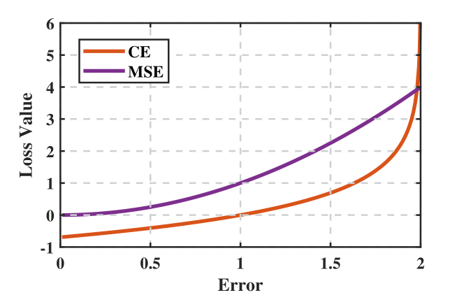
Figure 1: Loss curves of $\mathcal{L}_{CE}(t,e)$ and $\mathcal{L}_{MSE}(e)$ ($t=1$).

Moreover, currently in a variety of neural networks for classification, tanh and sigmoid transformation is widely used in output layers. According to [29], these classifiers with continuous errors, such as logistic regression and neural networks, are named as regression-like classifiers. On the contrary, those with discrete errors are named as non-regression-like classifiers, such as decision trees where the prediction is discrete label rather than continuous probability.

III Error Distribution Analysis

In this section, in the context of $\{0,1\}$-label coding scheme and logistic regression, we focus on analyzing the optimal error distribution $\rho_{E}(e)$ in the presence of outliers. Denoting the class prior probability by $p=P(T=1)$ and $q=1-p=P(T=0)$, one obtains the cumulative distribution function of error as follows

$$\begin{split}F_{E}(e)&=P(E\leqslant e)\;\\ &=pP(E\leqslant e|T=1)+qP(E\leqslant e|T=0)\;\\ &=pP(1-Y\leqslant e|T=1)+qP(-Y\leqslant e|T=0)\;\\ &=p(1-F_{Y|1}(1-e))+q(1-F_{Y|0}(-e))\;\\ &=1-pF_{Y|1}(1-e)-qF_{Y|0}(-e)\;\\ \end{split}$$ (6)

The error PDF is obtained by differentiation of $F_{E}(e)$ as

$$f_{E}(e)=pf_{Y|1}(1-e)+qf_{Y|0}(-e)$$ (7)

Assume that the samples of 0 class and 1 class are of two multivariate Gaussian distributions, $X|_{T=0}\sim\mathcal{N}(x;\mu_{0},\varSigma_{0})$ and $X|_{T=1}\sim\mathcal{N}(x;\mu_{1},\varSigma_{1})$, respectively. Given the boundary parameter $\omega$, then $\omega^{\prime}X|_{T}$ is of a univariate Gaussian distribution $\mathcal{N}(\omega^{\prime}x;\omega^{\prime}\mu_{T},\omega^{\prime}\varSigma_{T}\omega)$. To obtain the PDF of the univariate random variable $Y|_{T}=1/(1+\exp(-\omega^{\prime}X|_{T}))$, we give the following well-known theorem.

Theorem 2: Assume $f_{X}(x)$ is the PDF of a random variable $X$, and $\vartheta(x)$ is a monotonic and differentiable function. If $g_{Y}(y)$ is the PDF of $Y=\vartheta(X)$ and $\vartheta^{\prime}(x)\neq 0$, $\forall x\in X$, then

$$g_{Y}(y)=\begin{cases}\frac{f_{X}(\vartheta^{-1}(y))}{|\vartheta^{\prime}(\vartheta^{-1}(y))|}\,\,\,\,\text{inf}\vartheta(x)<y<\text{sup}\vartheta(x)\\ 0\,\,\,\,\,\,\,\,\,\,\,\,\,\,\,\,\,\,\,\,\,\,\,\,\,\,\,\,\,\text{otherwise}\\ \end{cases}$$ (8)

where $x=\vartheta^{-1}(y)$ is the inverse function of $y=\vartheta(x)$.$\hfill\blacksquare$ Since the sigmoid function satisfies the above conditions, one can obtain the PDF of $Y|_{T}$ as

$$f_{Y|T}(y)=\frac{\exp(-\frac{(\log(\frac{y}{1-y})-\omega^{\prime}\mu_{T})^{2}}{2\omega^{\prime}\varSigma_{T}\omega})}{\sqrt{2\pi\omega^{\prime}\varSigma_{T}\omega}}$$ (9)

where $0<y<1$. This PDF can be viewed as a nonlinear scaling on the horizontal axis of Gaussian distribution, and hence it is single-peak as well. Since the optimal parameter aims to achieve minimum misclassification rate, it is supposed that most of the predicted $Y|_{T}$ are as close to the corresponding $T$ as possible, to say the distribution peak of $f_{Y|1}(y)$ and $f_{Y|0}(y)$ to be close to $1$ and $0$, respectively. Intuitive function curves with specific $\omega^{\prime}\mu_{T}$ and $\omega^{\prime}\varSigma_{T}\omega$ are given in Fig. 2(a) with solid lines. If adverse outliers happen to $X|_{T}$, the corresponding prediction will approach the opposite, since this is what outlier means. That is to say, for example, $f_{Y|1}(y)$ will emerge a small peak near $0$, and vice versa for $f_{Y|0}(y)$. The distributions caused by outliers are illustrated in dashed lines in Fig. 2(a). Substituting (9) into (7), one can obtain

$$\begin{split}f_{E}(e)=&\frac{p}{\sqrt{2\pi\omega^{\prime}\varSigma_{1}\omega}}\exp(-\frac{(\log(\frac{1-e}{e})-\omega^{\prime}\mu_{1})^{2}}{2\omega^{\prime}\varSigma_{1}\omega})\;\\ +&\frac{q}{\sqrt{2\pi\omega^{\prime}\varSigma_{0}\omega}}\exp(-\frac{(\log(\frac{-e}{1+e})-\omega^{\prime}\mu_{0})^{2}}{2\omega^{\prime}\varSigma_{0}\omega})\;\\ \end{split}$$ (10)

which is plotted with solid lines in Fig. 2(b) with the same specific $\omega^{\prime}\mu_{T}$ and $\omega^{\prime}\varSigma_{T}\omega$ as above, and the effects of outliers are shown with dashed lines as well. One can observe three significant peaks on $\{0,-1,1\}$.

Not only Gaussian cases but also others usually lead to a similar $f_{E}(e)$. Even in the cases where $X|_{T}$ is of multi-peak distribution, i.e. $\omega^{\prime}X|_{T}$ is multi-peak, $f_{E}(e)$ could be probably similar. The reason is, $\omega^{\prime}X|_{T}$ distributed on $(-\infty,\infty)$ is squeezed to $Y|_{T}\in(0,1)$ by sigmoid, and thus multiple peaks could be close enough so that they can be viewed as one peak. Moreover, the above arguments hold for other regression-like classifiers as well, since as stated before, the predicted $Y|_{T}$ is supposed to be distributed close to the corresponding $T$ in any kind of regression-like classifiers.

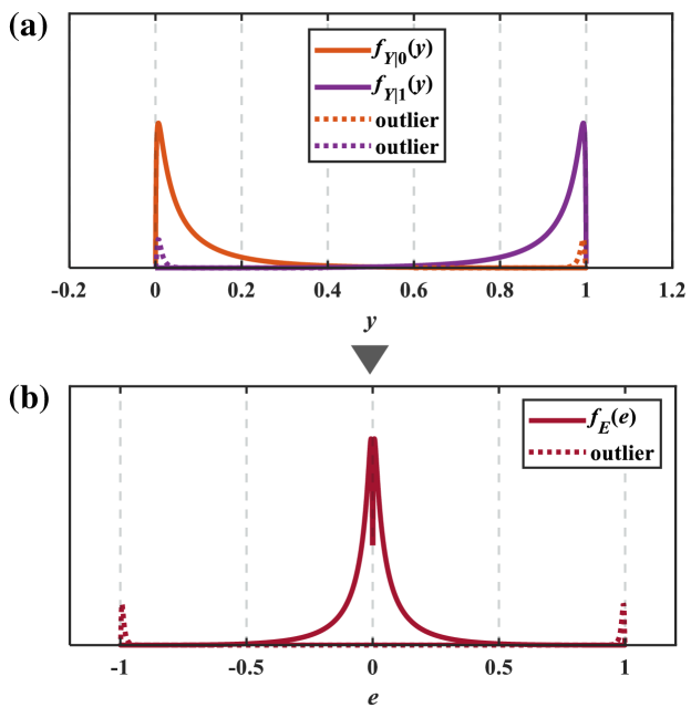
Figure 2: Illustrative function curves of (a)$f_{Y|T}(y)$ and (b)$f_{E}(e)$ ($\omega^{\prime}\mu_{0}=-5$, $\omega^{\prime}\mu_{1}=5$, $\omega^{\prime}\varSigma_{0}\omega=\omega^{\prime}\varSigma_{1}\omega=5$, $p=q=0.5$).

Now we focus on giving the formalization of the desired three-peak distribution $\rho_{E}(e)$. For clarity, supposing that class $0$ stands for negative and class $1$ means positive, we denote those outliers that lie in the positive side but are assigned with negative labels as false negative (FN) outliers, and vice versa as false positive (FP) outliers. Note that $x_{i}$ is predicted correctly if the corresponding $|e_{i}|<0.5$, otherwise wrongly. Therefore, the errors brought by inliers would be less than $0.5$ in the sense of absolute value since they are supposed to be classified correctly. On the other hand, FN outliers result in errors belonging to $(-1,-0.5)$, and FP outliers lead to errors belonging to $(0.5,1)$. For simplicity, we assume that each peak is close enough to a Dirac-$\delta$ function so that the density of the desired error PDF is zero beyond the three peaks. As a result, $\rho_{E}(e)$ is denoted as

$$\rho_{E}(e)=\begin{cases}\zeta_{0}\,\,\,\,\,\,\,\,\,\,\,\,\,\,\,\,e=0\\ \zeta_{-1}\,\,\,\,\,\,\,\,\,\,\,\,e=-1\\ \zeta_{1}\,\,\,\,\,\,\,\,\,\,\,\,\,\,\,\,e=1\\ 0\,\,\,\,\,\,\,\,\,\,\,\,\,\,\,\,\,\,\,\text{otherwise}\\ \end{cases}$$ (11)

where $\zeta_{i}$ ($i=0,-1,1$) denotes the corresponding density for each peak. One may have noticed that $\zeta_{i}$ is closely related to the proportion of each type of samples. To be specific, $\zeta_{0}$ is the proportion of inliers since the corresponding peak results from those samples that are supposed to be classified correctly. Similarly, $\zeta_{1}$ (or $\zeta_{-1}$) is the proportion of FP (or FN) outliers.

If, as in cross entropy loss $\mathcal{L}_{CE}(t,e)$, a large penalty is imposed to a large error, outliers will be dominant in the learning process, thus making it difficult to learn through meaningful samples. The inspiration of this study is that, the optimal parameter will result in an error distribution that holds three significant peaks at $\{0,-1,1\}$ by inliers, FN outliers, and FP outliers, respectively. If a classifier is designed to realize a similar error distribution, it can probably achieve satisfactory robust classification.

IV MEE for Classification

IV-A Introduction of MEE Criterion

The minimum error entropy (MEE) criterion has been proved to be robust in many machine learning tasks. MEE aims to minimize the Renyi’s $\alpha$ entropy of prediction error, which is introduced as a generalization of Shannon’s entropy [22]. Renyi’s $\alpha$ entropy, or called Renyi’s entropy of $\alpha$-order, is defined as

$${{H}_{R,\alpha}}\left(f_{E}(e)\right)\triangleq\frac{1}{1-\alpha}\log\int{f_{E}^{\alpha}\left(e\right)de}$$ (12)

in which $f_{E}(e)$ denotes the PDF of prediction error. The information potential is defined as the term in the logarithm

$${I_{\alpha}}\left(f_{E}(e)\right)\triangleq\int{f_{E}^{\alpha}\left(e\right)de=E}\left[f_{E}^{\alpha-1}\left(e\right)\right]$$ (13)

where $E[\cdot]$ is the expectation operator. For simplicity, the parameter $\alpha$ is usually set at $\alpha=2$. Because the logarithm is monotonically increasing, minimizing Renyi’s quadratic entropy ${{H}_{R,2}}\left(f_{E}(e)\right)$ is equal to maximizing the quadratic information potential ${I_{2}}\left(f_{E}(e)\right)$

$$\begin{split}\min H_{R,2}\left(f_{E}(e)\right)&\Longleftrightarrow\max I_{2}\left(f_{E}(e)\right)\;\\ &\Longleftrightarrow\max E\left[f_{E}(e)\right]\;\\ \end{split}$$ (14)

Based on an empirical version of the quadratic information potential [22], one can obtain

$$\begin{split}\omega^{*}&=\mathop{arg\max}_{\omega\in\mathcal{W}}\hat{I}_{2}\left(f_{E}(e)\right)\;\\ &=\mathop{arg\max}_{\omega\in\mathcal{W}}E\left[\hat{f}_{E}(e)\right]=\mathop{arg\max}_{\omega\in\mathcal{W}}\frac{1}{N}\sum_{i=1}^{N}{\hat{f}_{E}\left(e_{i}\right)}\;\\ &=\mathop{arg\max}_{\omega\in\mathcal{W}}\frac{1}{N^{2}}\sum_{i=1}^{N}{\sum_{j=1}^{N}{\kappa_{\sigma}\left(e_{i}-e_{j}\right)}}\;\\ \end{split}$$ (15)

where $\hat{f}_{E}\left(\cdot\right)$ is the estimated error PDF by Parzen’s estimator [30, 31]

$$\hat{f}_{E}\left(e\right)=\frac{1}{N}\sum_{j=1}^{N}{\kappa_{\sigma}\left(e-e_{j}\right)}$$ (16)

and $\kappa_{\sigma}\left(\cdot\right)$ is the Gaussian kernel function with bandwidth $\sigma$

$${{\kappa}_{\sigma}}\left(x\right)=\frac{1}{\sqrt{2\pi}\sigma}\exp\left(-\frac{{{x}^{2}}}{2{{\sigma}^{2}}}\right)$$ (17)

One could view the PDF estimator $\hat{f}_{E}\left(\cdot\right)$ as an adaptive objective function since it changes with $\{e_{i}\}_{i=1}^{N}$, which is different from the conventional ones that are generally invariable. The adaptation is advantageous, which has been proved theoretically as well as confirmed numerically [22].

To alleviate the computational bottleneck caused by double summation in (LABEL:mee), quantization technique is implemented that the error PDF is estimated by a little part of samples but not the entirety, thus decreasing the number of inner summation [23]. As a result, the quantized MEE (QMEE) is expressed as

$$\begin{split}\omega^{*}&=\mathop{arg\max}_{\omega\in\mathcal{W}}\hat{I}_{2}^{Q}\left(f_{E}(e)\right)\;\\ &=\mathop{arg\max}_{\omega\in\mathcal{W}}E\left[\hat{f}_{E}^{Q}(e)\right]=\mathop{arg\max}_{\omega\in\mathcal{W}}\frac{1}{N}\sum_{i=1}^{N}{\hat{f}_{E}^{Q}\left(e_{i}\right)}\;\\ &=\mathop{arg\max}_{\omega\in\mathcal{W}}\frac{1}{N^{2}}\sum_{i=1}^{N}{\sum_{j=1}^{N}{\kappa_{\sigma}\left(e_{i}-Q[e_{j}]\right)}}\;\\ &=\mathop{arg\max}_{\omega\in\mathcal{W}}\frac{1}{N^{2}}\sum_{i=1}^{N}{\sum_{j=1}^{M}{\varphi_{j}\kappa_{\sigma}\left(e_{i}-c_{j}\right)}}\;\\ \end{split}$$ (18)

where $\hat{I}_{2}^{Q}\left(f_{E}(e)\right)$ denotes the quantized quadratic information potential and $\hat{f}_{E}^{Q}(e)$ is the estimated error PDF based on some representative samples. $Q[\cdot]$ denotes a quantization operator that leads to a codebook $C=(c_{1},c_{2},...,c_{M})$, which means $Q[\cdot]$ is a function that maps each $\{e_{i}\}_{i=1}^{N}$ to one of $\{c_{j}\}_{j=1}^{M}$. The parameter $\varPhi=(\varphi_{1},\varphi_{2},...,\varphi_{M})$ denotes the number that how many samples are quantized to the corresponding word. Clearly one has $\sum_{j=1}^{M}{\varphi_{j}}=N$. Since $\{c_{j}\}_{j=1}^{M}$ is a representative description of $\{e_{i}\}_{i=1}^{N}$, we usually have $M\ll N$ and the complexity is thus decreased from $O(N^{2})$ to $O(MN)$. Proved by theoretical analysis and experimental results, QMEE can realize commensurate performance as the original one with proper quantization [23, 24]. In short, it is precisely because the codebook words $\{c_{j}\}_{j=1}^{M}$ are representative enough for the entirety $\{e_{i}\}_{i=1}^{N}$, that QMEE in (LABEL:qmee) can play the same effect as the original MEE in (LABEL:mee). In the context of univariate error, an adaptive quantization method was proposed in [24], which is summarized in Algorithm 1.

Algorithm 1 Procedure of Adaptive Quantization

1:Input samples $\left\{{{x}_{i}}\right\}_{\text{i}=1}^{N}$. Compute the range $L=\max(x_{i})-\min(x_{i})$.

2:Parameter setting: quantization threshold $\varepsilon$. Usually $\varepsilon=0.05$.

3:Initialize ${{C}_{1}}=\left\{{{x}_{1}}\right\}$, where ${{C}_{i}}$ denotes the codebook at the ith iteration.

4:for $i=2,\cdots,N$ do

5:     Compute the minimum distance between ${{x}_{i}}$ and ${{C}_{i-1}}$: $\text{dis}\left({{x}_{i}},{{C}_{i-1}}\right)=\underset{1\leq j\leq\left|{{C}_{i-1}}\right|}{\mathop{\min}}\left|{{x}_{i}}-{{C}_{i-1}}\left({{j}}\right)\right|$ where ${{C}_{i-1}}\left(j\right)$ denotes the jth element of ${{C}_{i-1}}$, and $\left|{{C}_{i-1}}\right|$ stands for the size of ${{C}_{i-1}}$.

6:     if $\text{dis}\left({{x}_{i}},{{C}_{i-1}}\right)\leq\varepsilon L$ then

7:         Keep the codebook unchanged: ${{C}_{i}}={{C}_{i-1}}$ and quantize ${{x}_{i}}$ to the closest code word: $Q\left[{{x}_{i}}\right]={{C}_{i-1}}\left({{j}^{*}}\right)$, where ${j}^{*}=\underset{1\leq j\leq\left|{{C}_{i-1}}\right|}{\mathop{\arg\min}}\left|{{x}_{i}}-{{C}_{i-1}}\left({{j}}\right)\right|$.

8:     else

9:         Update the codebook: ${{C}_{i}}=\left\{{{C}_{i-1}},{{x}_{i}}\right\}$ and quantize ${{x}_{i}}$ to itself: $Q\left[{{x}_{i}}\right]={{x}_{i}}$.

10:     end if

11:end for

12:Output $\left\{Q\left[{{x}_{i}}\right]\right\}_{i=1}^{N}$.

Entropy provides a PDF concentration measure that higher concentration implies lower entropy, which is the initial motivation to use entropic risk functionals. For continuous distributions, the local minimum value of ${{H}_{R,2}}\left(f_{E}(e)\right)$ corresponds to a PDF represented by several continuous Dirac-$\delta$ functions, a Dirac-$\delta$ comb. When all errors are zero, a single Dirac-$\delta$ at the origin for the error PDF can be achieved, leading to the ideal situation, $f_{E}(e)=0|_{e\neq 0}$. This demands a learning machine, in iterative training, to indeed guarantee the convergence of the error PDF towards a single Dirac-$\delta$ at the origin.

The robustness of MEE can be briefly explained as follows. In the training process with regular samples, MEE ensures most of errors are close to zero so as to approach a Dirac-$\delta$ function at the origin. If outliers happen, the error PDF will not only hold a main peak at the origin as before, but also generate small peaks at large errors caused by outliers. This kind of distribution, as mentioned earlier, is a local minimum for MEE as well. In addition, it can be interpreted from the perspective of equation (LABEL:mee) and (17). For a large error caused by outlier, its effect on the maximized term $\hat{I}_{2}\left(f_{E}(e)\right)$ in (LABEL:mee) is weakened since the Gaussian kernel function in (17) is bounded, which can saturate the summation term $\kappa_{\sigma}\left(e_{i}-e_{j}\right)$ of the last line in (LABEL:mee). Theoretical insights of robustness are provided in [22, 32].

IV-B MEE for Classification

Through the brief introduction, MEE is supposed to be appropriate for robust classification, since the optimal error PDF with outliers is a three-peak distribution, which is exactly an optimal for MEE. Nevertheless, compared to regression, one will encounter additional suffering in the implementation of MEE for classification. In the literature, one valuable study explored the implementation of MEE for different classifiers [29]. As stated, “MEE is harder for classification than for regression”. The main difficulties are summarized as follows.

In binary classification, according to [29], the purpose of MEE can be decomposed as

$$\begin{split}&\min H_{R,2}\left(f_{E}(e)\right)\;\\ &\Longleftrightarrow\max I_{2}\left(f_{E}(e)\right)\;\\ &\Longleftrightarrow\max(p^{2}I_{2}\left(f_{Y|1}(1-e)\right)+q^{2}I_{2}\left(f_{Y|0}(-e)\right))\;\\ \end{split}$$ (19)

in which the class-conditional property causes the difficulty. Recall that class-conditional distributions, entropies, and information potentials depend on the model parameter $\omega$, although this dependency has been omitted for simpler notation. Minimizing $H_{R,2}\left(f_{E}(e)\right)$ implies maximizing the sum of $p^{2}I_{2}\left(f_{Y|1}(1-e)\right)$ and $q^{2}I_{2}\left(f_{Y|0}(-e)\right)$, both of which are functions with respect to $\omega$. Thus, it is difficult to say about the minimum of $H_{R,2}\left(f_{E}(e)\right)$ since it depends on $p$, $q$, $f_{Y|1}$, and $f_{Y|0}$ simultaneously. One has to consider each class-conditional distribution individually and study them together with the weights $p$, $q$ to achieve minor $H_{R,2}\left(f_{E}(e)\right)$ as possible. By contrast, in regression tasks, $f_{E}(e)$ is not divided into several class-conditional parts but as a whole, which is much easier to deal with.

The above interpretation seems not intuitive that how MEE could fail for classification, so we provide a specific scenario. Sometimes MEE based classifiers may predict all samples as the same class with large confidence. For example, suppose that each predicted probability $\{y_{i}\}_{i=1}^{N}$ is close to $0$. Thus, the errors from 0-class samples will be close to $0$, while those from 1-class samples will be close to $1$, resulting in an $f_{E}(e)$ with two approximate Dirac-$\delta$ functions at $\{0,1\}$, respectively. The basic explanation was already given as before: any Dirac-$\delta$ comb achieves local minimum entropy. Note that when a similar case occurs, the classification accuracy could be even the chance level. This instability of MEE for classification is in particular explained in [29] with illustrative examples, which is verified in this paper as well by experimental results.

V Restricted MEE

The instability above inspires that, only focusing on minimizing entropy, i.e. maximizing information potential in (LABEL:mee), is not enough. From now on, getting rid of the MEE framework temporarily, we first focus on driving the error PDF obtained by the training process towards the optimal three-peak distribution $\rho_{E}(e)$ in (11). To make two distributions as similar as possible, a basic idea is to maximize a similarity measure between their PDFs. A quantity of similarity measures for PDF exist in the literature, for which [33] provides a comprehensive survey. In this paper we utilize the fundamental inner product to measure the similarity between distributions, which is generalized from its use for vectors [34, 35]. The inner-product similarity between two continuous PDFs $f_{X}(x)$ and $g_{X}(x)$ is computed as

$$\left\langle f_{X}(x),g_{X}(x)\right\rangle=\int_{X}{f_{X}(x)g_{X}(x)dx}$$ (20)

Now one can maximize this similarity measure between the error PDF $f_{E}(e)$ and the desired distribution $\rho_{E}(e)$ as

$$\begin{split}&\max\left\langle f_{E}(e),\rho_{E}(e)\right\rangle\;\\ &\Longleftrightarrow\max\int_{X}{f_{E}(e)\rho_{E}(e)dx}\;\\ &\Longleftrightarrow\max\zeta_{0}f_{E}(0)+\zeta_{-1}f_{E}(-1)+\zeta_{1}f_{E}(1)\;\\ \end{split}$$ (21)

the last equality of which arises from that $\rho_{E}(e)$ in (11) is always zero except when $e=0,-1,$ or $1$. In practice, one maximizes the similarity using the empirical version as

$$\begin{split}\omega^{*}&=\mathop{arg\max}_{\omega\in\mathcal{W}}\left\langle\hat{f}_{E}(e),\rho_{E}(e)\right\rangle\;\\ &=\mathop{arg\max}_{\omega\in\mathcal{W}}\zeta_{0}\hat{f}_{E}(0)+\zeta_{-1}\hat{f}_{E}(-1)+\zeta_{1}\hat{f}_{E}(1)\;\\ &=\mathop{arg\max}_{\omega\in\mathcal{W}}{\left(\begin{array}[]{c}\zeta_{0}\frac{1}{N}\sum_{i=1}^{N}{\kappa_{\sigma}\left(0-e_{i}\right)}\\ +\zeta_{-1}\frac{1}{N}\sum_{i=1}^{N}{\kappa_{\sigma}\left(-1-e_{i}\right)}\\ +\zeta_{1}\frac{1}{N}\sum_{i=1}^{N}{\kappa_{\sigma}\left(1-e_{i}\right)}\\ \end{array}\right)}\;\\ &=\mathop{arg\max}_{\omega\in\mathcal{W}}\frac{1}{N}\sum_{i=1}^{N}{\left(\begin{array}[]{c}\zeta_{0}\kappa_{\sigma}\left(e_{i}\right)\\ +\zeta_{-1}\kappa_{\sigma}\left(e_{i}+1\right)\\ +\zeta_{1}\kappa_{\sigma}\left(e_{i}-1\right)\\ \end{array}\right)}\;\\ &=\mathop{arg\max}_{\omega\in\mathcal{W}}\frac{1}{N^{2}}\sum_{i=1}^{N}{\left(\begin{array}[]{c}N\zeta_{0}\kappa_{\sigma}\left(e_{i}\right)\\ +N\zeta_{-1}\kappa_{\sigma}\left(e_{i}+1\right)\\ +N\zeta_{1}\kappa_{\sigma}\left(e_{i}-1\right)\\ \end{array}\right)}\;\\ \end{split}$$ (22)

One may have noticed the comparability between this form and QMEE, since this formula (LABEL:rmee2) can be regarded as a special case of QMEE in (LABEL:qmee) when the codebook $C=(0,-1,1)$, the corresponding quantization number $\varPhi=(N\zeta_{0},N\zeta_{-1},N\zeta_{1})$, and obviously $M=3$. Note that the derivation of formula (LABEL:rmee2) has nothing to do with the MEE framework originally since it aims to maximize the inner-product similarity between the error PDF $f_{E}(e)$ and the desired distribution $\rho_{E}(e)$. That is to say, from another point of view, we obtain a consequence that are closely related to MEE.

Now, returning back to MEE framework, we will interpret the meaning of formula (LABEL:rmee2). From the perspective of principle, QMEE aims to concentrate the prediction errors as close as possible to each $\{c_{j}\}_{j=1}^{M}$ to achieve a relatively narrow error distribution, in which $\{\varphi_{j}\}_{j=1}^{M}$ act as weight parameters. We can expect that if the codebook is assigned with some specific values, QMEE will focus the training errors close to these positions with certain weights $\varPhi$. With this consideration, we implement QMEE with a predetermined codebook $C=(0,-1,1)$, the purpose of which is to restrict errors on these three positions, avoiding the undesirable double-peak training consequence. QMEE with a restricted codebook, restricted MEE (RMEE) in short, is proposed by using the predetermined codebook $C=(0,-1,1)$, which is denoted as

$$\begin{split}\omega^{*}&=\mathop{arg\max}_{\omega\in\mathcal{W}}\hat{I}_{2}^{R}\left(f_{E}(e)\right)\;\\ &=\mathop{arg\max}_{\omega\in\mathcal{W}}\frac{1}{N^{2}}\sum_{i=1}^{N}{\left(\begin{array}[]{c}\varphi_{0}\kappa_{\sigma}\left(e_{i}\right)\\ +\varphi_{-1}\kappa_{\sigma}\left(e_{i}+1\right)\\ +\varphi_{1}\kappa_{\sigma}\left(e_{i}-1\right)\\ \end{array}\right)}\;\\ \end{split}$$ (23)

where $\hat{I}_{2}^{R}\left(f_{E}(e)\right)$ denotes the restricted quadratic information potential and we have $\varPhi=(\varphi_{0},\varphi_{-1},\varphi_{1})=(N\zeta_{0},N\zeta_{-1},N\zeta_{1})$, which denotes the corresponding number for each quantization word $C=(0,-1,1)$. One can see obviously that the essential difference between QMEE and the proposed RMEE is, the codebook $C$ of the former is obtained by a data-driven method as in Algorithm 1, which aims to make the elements $\{c_{j}\}_{j=1}^{M}$ as representative to the entirety as possible, while the latter’s is predetermined, which aims to drive the error PDF $f_{E}(e)$ towards the desired one $\rho_{E}(e)$.

Now, through the above interpretations, two perspectives for the proposed RMEE are summarized as follows.

1: RMEE can be regarded as maximizing the inner-product similarity between the error PDF $f_{E}(e)$ and the desired three-peak distribution $\rho_{E}(e)$.

2: RMEE can also be viewed as a special case of QMEE that the codebook is predetermined as $C=(0,-1,1)$, which aims to concentrate errors on these three locations as possible.

In prediction (or testing), the method of labeling a sample is the same as in traditional methods that use the sigmoid transformation. Given the resultant model parameter, one first computes the probability $y_{i}$ for each sample according to the model. For example, in logistic regression, one has $y_{i}=1/(1+\exp(-\omega^{\prime}x_{i}))$. Then, one is supposed to label the sample $x_{i}$ with class 1 if the corresponding $y_{i}>0.5$, otherwise with class 0.

In the following, for the proposed RMEE, we discuss about its optimization, convergence analysis, and how to determine the hyper-parameters.

V-A Optimization

As seen in (LABEL:rmee3), the Gaussian kernel function will bring non-convexity in optimization, not to mention the implicit sigmoid transformation which is intractable particularly. Here we utilize the half-quadratic (HQ) technique to solve this problem, which is often used to solve ITL optimization issues [36, 37, 38, 39]. To derive the HQ-based optimization for (LABEL:rmee3), we first give the following theorem.

Theorem 3: Define a convex function $g(v)=-v\log(-v)+v$, where $v<0$. Based on the conjugate function theory [40], one has

$$\exp(-\frac{(t-y)^{2}}{2\sigma^{2}})=\mathop{\sup}_{v<0}\{v\frac{(t-y)^{2}}{2\sigma^{2}}-g(v)\}$$ (24)

where the supremum is achieved at $v=-\exp(-\frac{(t-y)^{2}}{2\sigma^{2}})<0$. See the proof in [38, 39].$\hfill\blacksquare$

Thus the form of RMEE in (LABEL:rmee3) can be rewritten as

$$\begin{split}&\omega^{*}=\mathop{arg\max}_{\omega\in\mathcal{W}}\sum_{i=1}^{N}{\left(\begin{array}[]{c}\varphi_{0}\mathop{\sup}_{u_{i}<0}\{u_{i}\frac{e_{i}^{2}}{2\sigma^{2}}-g(u_{i})\}\\ +\varphi_{-1}\mathop{\sup}_{v_{i}<0}\{v_{i}\frac{(e_{i}+1)^{2}}{2\sigma^{2}}-g(v_{i})\}\\ +\varphi_{1}\mathop{\sup}_{s_{i}<0}\{s_{i}\frac{(e_{i}-1)^{2}}{2\sigma^{2}}-g(s_{i})\}\\ \end{array}\right)}\;\\ &=\mathop{arg\max}_{\omega\in\mathcal{W},u_{i}<0,v_{i}<0,s_{i}<0}\sum_{i=1}^{N}{\left(\begin{array}[]{c}\varphi_{0}(u_{i}\frac{e_{i}^{2}}{2\sigma^{2}}-g(u_{i}))\\ +\varphi_{-1}(v_{i}\frac{(e_{i}+1)^{2}}{2\sigma^{2}}-g(v_{i}))\\ +\varphi_{1}(s_{i}\frac{(e_{i}-1)^{2}}{2\sigma^{2}}-g(s_{i}))\\ \end{array}\right)}\;\\ &=\mathop{arg\max}_{\omega\in\mathcal{W},u_{i}<0,v_{i}<0,s_{i}<0}J_{R}(\omega,u_{i},v_{i},s_{i})\;\\ \end{split}$$ (25)

where $1/(N^{2}\sqrt{2\pi}\sigma)$ is omitted in the second equality since it is a constant with fixing the kernel bandwidth $\sigma$. Note that although the model parameter $\omega$ is implicit in $J_{R}(\omega,u_{i},v_{i},s_{i})$ in (LABEL:rmee_hq_1), it has a direct influence on $e_{i}$. Now one can optimize $J_{R}(\omega,u_{i},v_{i},s_{i})$ by alternate optimization on $\omega$, $u_{i}$, $v_{i}$, and $s_{i}$, respectively. To be specific, in the kth iteration with the current errors $\{e_{i}\}_{i=1}^{N}$, one first optimizes

$$\begin{split}&(u_{i}^{k},v_{i}^{k},s_{i}^{k})\;\\ &=\mathop{arg\max}_{u_{i}<0,v_{i}<0,s_{i}<0}\sum_{i=1}^{N}{\left(\begin{array}[]{c}\varphi_{0}(u_{i}\frac{e_{i}^{2}}{2\sigma^{2}}-g(u_{i}))\\ +\varphi_{-1}(v_{i}\frac{(e_{i}+1)^{2}}{2\sigma^{2}}-g(v_{i}))\\ +\varphi_{1}(s_{i}\frac{(e_{i}-1)^{2}}{2\sigma^{2}}-g(s_{i}))\\ \end{array}\right)}\;\\ &=\mathop{arg\max}_{u_{i}<0,v_{i}<0,s_{i}<0}J_{R1}(u_{i},v_{i},s_{i})\;\\ \end{split}$$ (26)

According to (24), the closed-form solution of (LABEL:hq_op_1) is

$$\begin{array}[]{c}u_{i}^{k}=-\exp(-\frac{e_{i}^{2}}{2\sigma^{2}})<0\\ v_{i}^{k}=-\exp(-\frac{(e_{i}+1)^{2}}{2\sigma^{2}})<0\\ s_{i}^{k}=-\exp(-\frac{(e_{i}-1)^{2}}{2\sigma^{2}})<0\\ (i=1,2,...,N)\\ \end{array}$$ (27)

Second, after obtaining the optimal $(u_{i}^{k},v_{i}^{k},s_{i}^{k})$ in the kth iteration, one obtains $\omega^{k}$ by solving the following optimization

$$\begin{split}\omega^{k}&=\mathop{arg\max}_{\omega\in\mathcal{W}}\sum_{i=1}^{N}{\left(\begin{array}[]{c}\varphi_{0}(u_{i}\frac{e_{i}^{2}}{2\sigma^{2}}-g(u_{i}))\\ +\varphi_{-1}(v_{i}\frac{(e_{i}+1)^{2}}{2\sigma^{2}}-g(v_{i}))\\ +\varphi_{1}(s_{i}\frac{(e_{i}-1)^{2}}{2\sigma^{2}}-g(s_{i}))\\ \end{array}\right)}\;\\ &=\mathop{arg\max}_{\omega\in\mathcal{W}}\sum_{i=1}^{N}{\left(\begin{array}[]{c}\varphi_{0}u_{i}(t_{i}-y_{i})^{2}\\ +\varphi_{-1}v_{i}(t_{i}+1-y_{i})^{2}\\ +\varphi_{1}s_{i}(t_{i}-1-y_{i})^{2}\\ \end{array}\right)}\;\\ &=\mathop{arg\max}_{\omega\in\mathcal{W}}J_{R2}(\omega)\;\\ \end{split}$$ (28)

in which $g(\cdot)$ and $1/2\sigma^{2}$ are omitted since they are constants in this step. Note that for different regression-like classifiers, the form of $y_{i}$ is different. For example, in logistic regression one has $y_{i}=1/(1+\exp(-\omega^{\prime}x_{i}))$, while $y_{i}$ will be sophisticated in neural networks since they are of hierarchical structures. Nevertheless, even in neural networks, one can always optimize $J_{R2}(\omega)$ in (28) with the prominent back-propagation technique [41] and gradient-based optimization, since the objective function $J_{R2}(\omega)$ is continuous and differentiable. Here we give the derivation in the context of logistic regression, in which the gradient of $J_{R2}(\omega)$ in (28) is

$$\begin{split}&\frac{\partial J_{R2}(\omega)}{\partial\omega}=\sum_{i=1}^{N}{\left(\begin{array}[]{c}\varphi_{0}u_{i}\frac{\partial(t_{i}-y_{i})^{2}}{\partial\omega}\\ +\varphi_{-1}v_{i}\frac{\partial(t_{i}+1-y_{i})^{2}}{\partial\omega}\\ +\varphi_{1}s_{i}\frac{\partial(t_{i}-1-y_{i})^{2}}{\partial\omega}\\ \end{array}\right)}\;\\ &=-2\sum_{i=1}^{N}{\left(\begin{array}[]{c}\varphi_{0}u_{i}e_{i}\\ +\varphi_{-1}v_{i}(e_{i}+1)\\ +\varphi_{1}s_{i}(e_{i}-1)\\ \end{array}\right)x_{i}y_{i}(1-y_{i})}\;\\ \end{split}$$ (29)

Then one can use gradient-based or momentum-based optimization, such as the popular and efficient Adam [42], to obtain $\omega^{k}$ for (28). The HQ-based optimization for RMEE is summarized in Algorithm 2. Note that in (LABEL:hq_op_1)(27)(28)(LABEL:grad), we omit the superscript k somewhere for the reason of clarity.

Algorithm 2 HQ-based Optimization for RMEE

1:Input: training samples $\{x_{i},t_{i}\}_{i=1}^{N}$; initial model parameter $\omega$; hyper-parameters $\sigma$, $\varPhi=(\varphi_{0},\varphi_{-1},\varphi_{1})$; a small positive value $\varsigma$

2:Output: model parameter $\omega$

3:repeat

4:     Initialize $converged=$ FALSE;

5:     Compute the errors $\{e_{i}\}_{i=1}^{N}$ at the current model parameter $\omega$;

6:     Update $(u_{i},v_{i},s_{i})$ with (27);

7:     Update $\omega$ with (28) by gradient-based or momentum-based optimization;

8:     if  the difference of the objective function in (LABEL:rmee3) is smaller than $\varsigma$ then

9:         $converged=$ TRUE

10:     end if

11:until $converged==$ TRUE

V-B Convergence Analysis

One may be concerned about whether Algorithm 2 can converge to a local maximum. Actually, convergence of HQ-based optimization can be easily proved as

$$\begin{split}J_{R}(\omega^{k-1},u_{i}^{k-1},v_{i}^{k-1},s_{i}^{k-1})&\leqslant J_{R}(\omega^{k-1},u_{i}^{k},v_{i}^{k},s_{i}^{k})\;\\ &\leqslant J_{R}(\omega^{k},u_{i}^{k},v_{i}^{k},s_{i}^{k})\;\\ \end{split}$$ (30)

in which the first inequality is established obviously according to (LABEL:hq_op_1)(27). To establish the second inequality, i.e. $J_{R}(\omega^{k-1},u_{i}^{k},v_{i}^{k},s_{i}^{k})\leqslant J_{R}(\omega^{k},u_{i}^{k},v_{i}^{k},s_{i}^{k})$, the following equivalent inequality is supposed to be established with fixing $(u_{i},v_{i},s_{i})=(u_{i}^{k},v_{i}^{k},s_{i}^{k})$

$$J_{R2}(\omega^{k-1})\leqslant J_{R2}(\omega^{k})$$ (31)

Thus, to guarantee the convergence of Algorithm 2, one could find it not necessary for $\omega$ to achieve maximum in (28). On the contrary, as long as we have $J_{R2}(\omega^{k-1})\leqslant J_{R2}(\omega^{k})$ at every iteration with fixing $(u_{i},v_{i},s_{i})=(u_{i}^{k},v_{i}^{k},s_{i}^{k})$, the inequality (30) is established, which guarantees the convergence of Algorithm 2. Therefore, for the optimization problem in (28), one only needs to consider whether the new $\omega^{k}$ achieves a larger objective function value than the previous $\omega^{k-1}$, i.e. $J_{R2}(\omega^{k-1})\leqslant J_{R2}(\omega^{k})$.

V-C Hyper-Parameters Determination

Now, we focus on solving the determination of hyper-parameters $\sigma$ and $\varPhi$ for the proposed RMEE.

The kernel bandwidth $\sigma$ plays a vital role in Parzen-window-based methods. The famous Silverman’s Rule was proposed in [30] for density estimation, which has been used in ITL methods [37]. However, this method is not always favorable for ITL methods [22, 23, 24]. Therefore, in this paper we use the conservative five-fold cross-validation to choose a proper $\sigma$ for RMEE.

Considering the determination of $\varPhi$, the optimal values are supposed to be the numbers of inliers, FN outliers, and FP outliers, corresponding to $\varphi_{0}$, $\varphi_{-1}$, and $\varphi_{1}$, respectively. However, this will be intractable unless we have prior information about the outlier proportion. To determine $\varPhi$ without any prior information, we utilize the following empirical method to obtain an approximate estimation of outlier proportion. We first use an initial $\varPhi^{\prime}=(\varphi_{0}^{\prime},\varphi_{-1}^{\prime},\varphi_{1}^{\prime})=(N,0,0)$, i.e. $\zeta_{0}=1$ and $\zeta_{-1}=\zeta_{1}=0$ in $\rho_{E}(e)$, and train the model by Algorithm 2, which means that we expect all samples in the training dataset to achieve minor errors. This will give a resultant model parameter $\omega$, by which we can obtain $\{e_{i}\}_{i=1}^{N}$ belonging to the continuous interval $(-1,1)$. Then we estimate the outlier proportion by assuming the correctly predicted samples, whose errors belong to $(-0.5,0.5)$, are inliers. On the other hand, the errors belonging to $(-1,-0.5)$ and $(0.5,1)$ correspond to FN and FP outliers, respectively. Formally, we have

$$\begin{split}&\varphi_{0}^{\prime\prime}=\#\left\{e_{i}\in\left(-0.5,0.5\right)\right\}\;\\ &\varphi_{-1}^{\prime\prime}=\#\left\{e_{i}\in\left(-1,-0.5\right)\right\}\;\\ &\varphi_{1}^{\prime\prime}=\#\left\{e_{i}\in\left(0.5,1\right)\right\}\;\\ \end{split}$$ (32)

where $\#\left\{\cdot\right\}$ indicates counting the samples that meet the condition. Obviously we have $\varphi_{0}^{\prime\prime}+\varphi_{-1}^{\prime\prime}+\varphi_{1}^{\prime\prime}=N$. With the new $\varPhi^{\prime\prime}=(\varphi_{0}^{\prime\prime},\varphi_{-1}^{\prime\prime},\varphi_{1}^{\prime\prime})$, train the model again by Algorithm 2 and obtain the result of RMEE.

The above procedure is in fact adaptive. When the training dataset does not contain outliers, it can be supposed that almost all sample are classified well, which means $\varphi_{-1}^{\prime\prime}$ and $\varphi_{1}^{\prime\prime}$ will be of small values. Thus in the following training with $\varPhi^{\prime\prime}$, we will still expect almost all examples to achieve zero errors. On the other hand, if there are outliers in training dataset, considerable errors will be outside $\left(-0.5,0.5\right)$. Then, $\varphi_{-1}^{\prime\prime}$ and $\varphi_{1}^{\prime\prime}$ can reflect the outlier proportion to some extent, since higher outlier proportion will generally lead to worse training results, i.e. larger $\varphi_{-1}^{\prime\prime}$ and $\varphi_{1}^{\prime\prime}$.

In addition, note that RMEE with the initial weights $\varPhi^{\prime}=(\varphi_{0}^{\prime},\varphi_{-1}^{\prime},\varphi_{1}^{\prime})=(N,0,0)$ is actually equivalent to the C-Loss, the state-of-the-art loss function for robust classification [38, 39, 43], which was proposed from the famous correntropy in ITL and aims to maximize the density of $f_{E}(e)$ at $e=0$. Hence, the proposed RMEE can be regarded as a more generalized form of C-Loss.

VI Experiments

For performance comparison, above all, it is principal to compare RMEE with QMEE to demonstrate necessity of the proposed restriction. Furthermore, we involve the C-Loss in comparison, which can be viewed as a special case of RMEE, when $\varPhi=(\varphi_{0},\varphi_{-1},\varphi_{1})=(N,0,0)$. In addition, the traditional CE and MSE are involved as well. Note that MSE is used with the sigmoid transformation. In order to solve the non-convexity problem caused by the use of MSE and sigmoid together, the advanced Adam [42] is used.

One may probably worry that there are too few algorithms for performance comparison. We would like to argue that:

1: As reviewed in Section I, there are a variety of approaches to realize robust classification, such as removing samples, relabeling samples, weighting samples, etc. What most of these methods have in common is that, the desired robustness is realized in the preprocessing stage before the model learns, rather than in learning processes. The proposed RMEE in this paper is a robust objective function for classification, which means RMEE realizes robustness exactly in the learning process. Therefore, it is not necessary to compare RMEE with those methods that achieve robustness outside the learning process. Even RMEE can be used with these methods together.

2: What should exactly be compared with RMEE are those robust objective functions for classification, among which C-Loss has been proved to be state-of-the-art. Unlike traditional bounded losses, which are usually truncated by hard threshold [10, 21], C-Loss is always differentiable, and its kernel size could realize adaptive approximation to various norms in different ranges. For comparisons between C-Loss and existing robust losses, see [38, 39, 43].

The performance indicator through this paper is the classification accuracy that is computed as (TP+TN)/(TP+TN+FP+FN). All the average accuracy and corresponding standard deviations are given by 100 Monte-Carlo independent repetitions. Note that as suggested in [2], to evaluate the robustness between different classifiers, it is preferable to only contaminate training dataset with outliers, while keeping the testing dataset from contamination. This policy has been widely recognized and practiced in the literature of robust machine learning. Therefore, in this paper, the outlier contamination is only aimed at the training datasets, while the testing datasets are unchanged.

VI-A Logistic Regression

We first generate linear toy examples which will be contaminated by attribute and label outliers, respectively, and then evaluate the robustness of logistic regression models based on different criteria. Similarly as in [15], we randomly produce 1,000 i.i.d. $x_{i}\sim\mathcal{N}(0,I_{d})$ as training samples, 1,000 i.i.d. $x_{i}\sim\mathcal{N}(0,I_{d})$ as testing samples, and a true solution $\omega^{*}\sim\mathcal{N}(0,I_{d})$, where $I_{d}$ is the unit matrix of dimension $d$. Then, for all the samples, the labels are assigned with $1$ if ${\omega^{*}}^{\prime}x_{i}\geqslant 0$, otherwise with $0$. The dimension is $20$, and all dimensions are relative to the task. The numbers of two classes are supposed to be equal because $\omega^{*}$ always passes through the center of symmetrical Gaussian-distributed samples. As a result, a rather clean dataset is completed.

VI-A1 Attribute Contamination

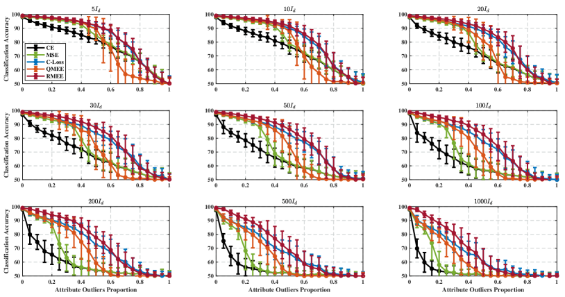
Figure 3: Average classification accuracy of the balanced-class toy dataset contaminated by attribute outliers.

Generally speaking, attribute contamination has no tendency for different classes since it usually occurs during the measurement process [2]. Therefore, the samples of two classes will sustain attribute contamination with equal probability. To contaminate this toy with attribute outliers, we randomly select some samples from the 1,000 training samples, and then replace their attribute values with a zero-mean Gaussian distribution with large covariance to simulate attribute outliers. For the covariance of Gaussian distribution for outliers, we consider several values, which are $5I_{d}$, $10I_{d}$, $20I_{d}$, $30I_{d}$, $50I_{d}$, $100I_{d}$, $200I_{d}$, $500I_{d}$, and $1000I_{d}$, respectively. The number of attribute outliers is denoted by outlier proportion, which is the ratio between the numbers of outliers and total training samples. It is appreciable that when outlier proportion is $1.0$, the accuracy will decrease to chance level because training samples do not carry any valid information. We increase the outlier proportion from $0$ to $1.0$ with a step $0.05$. The results are plotted in Fig. 3, where one can clearly observe that RMEE achieves the highest accuracy under almost all conditions, which highlights the superiority of MEE for robust classification when restricted by the predetermined codebook.

VI-A2 Label Contamination

Compared to attribute contamination, as stated in [4], samples from certain class could suffer label contamination with more probability. For example, control subjects in medical studies are more prone to be mislabeled [44]. In this paper, we use an asymmetric contamination that, in binary classification, only the samples of one class will be mislabeled whereas those of the other class will not, which requires stronger robustness [2, 4]. Moreover, in those cases prone to label contamination, the numbers of different classes are often unbalanced. Therefore, besides the above balanced-class toy dataset, we consider unbalanced-class case as well. To generate an unbalanced toy, a similar method as above is used, except that the mean of $x_{i}$ is shifted to $0.4$ instead, by which the amount of major class vs minor class is $(629.2\pm 86.9)$:$(370.8\pm 86.9)$.

For label outlier proportion, we use $Maj\rightarrow Min$ to denote that the labels of major-class samples flip to minor class, and $Min\rightarrow Maj$ for vice versa. First, for the balanced-class toy dataset, we increase the outlier proportion from $0$ to $0.5$ with a step $0.025$. Note that $Maj\rightarrow Min$ and $Min\rightarrow Maj$ are equivalent due to class balance. Next, for the unbalanced-class one, we increase $Maj\rightarrow Min$ or $Min\rightarrow Maj$ from $0$ to $0.5$ with a step $0.025$ bi-directionally while keeping the other as 0. The results are shown in Fig. 4, where one can find that RMEE achieves the highest accuracy in most cases as well.

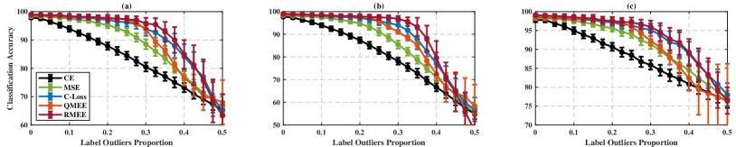
Figure 4: Average classification accuracy of the balanced-class and unbalanced-class toy datasets contaminated by label outliers (a) balanced-class toy, (b) unbalanced-class toy $Maj\rightarrow Min$, (c) unbalanced-class toy $Min\rightarrow Maj$.

VI-B Extreme Learning Machine

We then select some popular benchmark datasets from the UCI repository [45] and contaminate them artificially with attribute outliers and label outliers, respectively. The selected datasets are summarized in TABLE I. For each dataset, all the attributes only consist of numerical values. In the context of binary classification, we transform those multi-class datasets into several 2-class datasets. To realize this transformation, we build a new dataset that consists of the samples of one specific class, and assign the antagonistic label to the other samples. Thus, a dataset of $m$ classes is converted into $m$ datasets of binary class, which is known as one vs all. This helps analyze whether the classifier could extract effective pattern for each class. We randomly select $2/3$ samples for training, and the other $1/3$ samples act as testing samples.

TABLE I: Benchmark datasets summary.

No.	Dataset	Feature	Class Ratio
1	Statlog (Australian Credit Approval)	14	383 : 307
2	Balance Scale (l. vs all)	4	337 : 288
3	Balance Scale (r. vs all)	4	337 : 288
4	BUPA Liver Disorders	6	200 : 145
5	Connectionist (Sonar, Mines vs. Rocks)	60	111 : 97
6	Iris (set. vs all)	4	100 : 50
7	Iris (vir. vs all)	4	100 : 50
8	Breast Cancer Wisconsin (Original)	9	458 : 241
9	Breast Cancer Wisconsin (Diagnostic)	30	357 : 212
10	Wholesale Customers	7	298 : 142

In this subsection, for contaminated benchmark datasets, we use the extreme learning machine (ELM) [46] model for performance evaluation, which is a supervised single-hidden-layer neural network and initializes input weights and hidden layer biases randomly. The robust variant of ELM based on C-Loss was proposed in [39]. The number of nodes in the hidden layer is set as 50 in this paper.

VI-B1 Attribute Contamination

For training samples in each dataset, we first normalize each dimension to zero-mean and unit-variance, so that the diagonal elements of the covariance matrix of the training samples are all 1. Then, similarly, we randomly select some samples and replace their attribute values with a zero-mean Gaussian distribution with large covariance, which are $5I_{d}$, $20I_{d}$, $50I_{d}$, $100I_{d}$, $300I_{d}$, and $1000I_{d}$, respectively. Same as before, the ratio between numbers of outliers and entirety is denoted by the proportion, and the results are listed in TABLE II. The highest accuracy in each condition is marked in bold. The ‘Acoustic’ means that the training data is not contaminated in any way.

TABLE II: Average classification accuracy of benchmark datasets contaminated by attribute outliers.

Dataset 1		CE	MSE	C-Loss	QMEE	RMEE	Dataset 2		CE	MSE	C-Loss	QMEE	RMEE
Acoustic		85.3412	85.4808	86.0922	85.1921	86.8995	Acoustic		94.6905	94.6811	94.2130	93.8143	94.2067
$5I_{d}$	20%	84.6691	84.3992	85.8602	85.1454	86.6462	$5I_{d}$	20%	92.3706	94.6656	94.9222	93.4903	94.6587
	40%	83.9640	83.9368	85.7641	76.5939	86.0349		40%	89.3256	91.8122	92.5345	86.3221	93.6106
$20I_{d}$	20%	84.4759	84.6244	85.9563	81.5240	86.4890	$20I_{d}$	20%	91.8823	94.5962	93.9991	90.0144	94.9760
	40%	83.5499	84.2607	84.5717	77.4716	85.8427		40%	87.0992	91.6451	92.4876	77.5385	92.8413
$50I_{d}$	20%	84.3015	84.7896	85.7872	80.3843	85.7118	$50I_{d}$	20%	90.2872	94.0074	93.6400	86.6779	94.5144
	40%	83.2894	84.8434	84.8872	75.1528	85.0655		40%	83.4484	89.7837	91.1139	74.0913	92.0048
$100I_{d}$	20%	84.5147	84.9551	85.9757	80.8035	85.8472	$100I_{d}$	20%	88.9504	93.5338	93.8302	84.0377	94.6010
	40%	81.1712	84.3196	84.3645	73.2052	85.0262		40%	76.5753	85.2663	88.8492	71.5096	89.5481
$300I_{d}$	20%	83.2600	84.9286	85.0182	75.5808	86.0454	$300I_{d}$	20%	81.7947	91.5097	91.9393	80.3317	93.5769
	40%	73.2197	82.7930	82.2569	70.8908	84.0699		40%	63.4042	71.5518	82.9603	66.6971	83.3269
$1000I_{d}$	20%	79.3717	84.2168	84.4941	75.3688	85.3974	$1000I_{d}$	20%	66.6864	83.0303	87.3118	75.6346	90.0721
	40%	60.6157	73.1882	77.2149	65.3188	77.8079		40%	55.4845	57.0517	67.0551	60.8702	67.9327
Dataset 3		CE	MSE	C-Loss	QMEE	RMEE	Dataset 4		CE	MSE	C-Loss	QMEE	RMEE
Acoustic		94.9343	94.9031	95.0319	94.3782	95.1202	Acoustic		72.7316	72.2560	72.5066	68.0965	72.8596
$5I_{d}$	20%	92.1616	94.5170	94.4439	93.3189	94.9327	$5I_{d}$	20%	64.7649	67.1150	67.5085	63.5404	69.8596
	40%	88.7445	91.4719	92.1872	83.9432	93.1346		40%	61.5798	62.4558	62.7829	58.5088	65.1579
$20I_{d}$	20%	92.0175	94.2866	93.7551	93.0048	94.6971	$20I_{d}$	20%	64.2705	67.0410	67.2073	63.7105	67.7368
	40%	86.8134	91.5106	92.3579	81.9183	92.9808		40%	59.3699	61.0136	59.9025	56.8158	61.3070
$50I_{d}$	20%	90.8500	93.3372	93.3186	90.9663	94.0577	$50I_{d}$	20%	62.1117	65.3978	65.0258	61.7895	65.2281
	40%	82.4368	90.0990	91.0431	78.2452	91.9567		40%	57.9555	58.6776	58.7636	56.8333	59.7544
$100I_{d}$	20%	89.1367	93.4503	93.4003	87.6058	93.8798	$100I_{d}$	20%	59.6345	62.0637	61.7865	59.2105	62.1842
	40%	75.1375	85.3168	89.7191	76.7692	90.1202		40%	57.7224	58.0879	58.0280	53.6316	58.5526
$300I_{d}$	20%	81.1232	91.3057	92.1224	83.0962	93.3846	$300I_{d}$	20%	57.5348	59.0547	59.1582	58.7632	58.8772
	40%	63.2575	71.6601	80.7237	70.5961	81.1827		40%	57.6294	57.7364	57.0454	53.4649	57.7018
$1000I_{d}$	20%	65.9159	81.1820	88.5470	80.6346	89.6490	$1000I_{d}$	20%	57.6489	58.1530	58.1196	54.6404	58.1053
	40%	55.1541	57.4967	65.4652	60.8269	65.7644		40%	57.7166	57.7618	57.3507	52.5263	57.6053
Dataset 5		CE	MSE	C-Loss	QMEE	RMEE	Dataset 6		CE	MSE	C-Loss	QMEE	RMEE
Acoustic		77.0282	77.5908	77.7576	77.3712	77.5797	Acoustic		99.7893	99.2746	99.5171	99.0631	99.0408
$5I_{d}$	20%	73.7599	74.1754	75.8732	70.6087	75.9565	$5I_{d}$	20%	99.7838	99.3795	98.7406	97.5918	98.5306
	40%	71.9547	70.0328	74.0929	69.9565	74.9130		40%	99.5855	98.1407	98.5211	87.7347	98.6327
$20I_{d}$	20%	72.8445	72.7313	74.1694	70.1594	75.8841	$20I_{d}$	20%	99.6234	99.1297	99.0156	96.7143	97.6327
	40%	70.9818	70.0738	74.6192	69.1739	74.3188		40%	99.4411	98.6793	97.0664	86.3061	96.1224
$50I_{d}$	20%	72.2072	72.2641	74.2687	70.9275	75.7681	$50I_{d}$	20%	99.7710	98.8713	98.2464	95.6939	97.9592
	40%	70.9769	70.9091	74.1996	68.6087	74.8116		40%	97.1245	98.5852	97.7731	85.3469	95.6939
$100I_{d}$	20%	72.7967	72.5096	74.2348	71.8441	75.4783	$100I_{d}$	20%	99.7606	98.1226	97.0511	93.9388	97.2857
	40%	69.3462	70.1595	73.8919	68.0870	74.3333		40%	91.8587	98.1526	97.4333	84.9388	96.0612
$300I_{d}$	20%	70.4031	70.7418	72.6084	70.6232	73.6522	$300I_{d}$	20%	97.7551	98.8015	97.7083	89.3265	97.6122
	40%	68.0087	70.4738	72.5308	66.6973	71.6377		40%	73.3285	90.4130	93.9672	83.9388	95.2449
$1000I_{d}$	20%	70.8000	70.4146	72.9791	67.7681	72.1159	$1000I_{d}$	20%	83.2386	98.1099	96.6321	89.4286	94.6735
	40%	65.3351	69.6401	69.3089	65.1159	70.3913		40%	67.9696	75.8694	78.1879	79.5714	79.4082
Dataset 7		CE	MSE	C-Loss	QMEE	RMEE	Dataset 8		CE	MSE	C-Loss	QMEE	RMEE
Acoustic		96.2420	94.3650	94.7064	95.0000	95.0408	Acoustic		96.3070	95.1221	95.5036	95.5388	95.7500
$5I_{d}$	20%	93.9750	94.6976	94.3587	94.3854	95.0776	$5I_{d}$	20%	95.8097	95.5167	94.4502	94.7414	95.4698
	40%	89.9350	90.5405	91.9693	85.1633	92.5510		40%	95.3661	95.6059	94.7405	94.9009	95.5302
$20I_{d}$	20%	92.1655	92.6733	92.6554	90.9796	93.1837	$20I_{d}$	20%	95.9798	95.8572	94.4977	93.6881	95.8534
	40%	88.8540	90.6625	90.4983	84.0816	91.4898		40%	95.1232	95.6049	94.0459	92.7198	94.7716
$50I_{d}$	20%	90.4424	91.5963	91.1111	90.6531	91.9592	$50I_{d}$	20%	95.1250	94.4612	94.8319	91.4655	95.1595
	40%	83.6684	85.1672	88.0256	82.5306	88.2857		40%	93.2328	93.7414	92.8060	87.6810	92.3448
$100I_{d}$	20%	89.7892	90.7375	91.5391	88.5714	91.9388	$100I_{d}$	20%	94.7328	95.2586	94.0905	88.2026	95.3362
	40%	77.2352	83.2288	85.2843	80.6351	85.6939		40%	90.1379	91.9310	92.2629	81.3966	92.4543
$300I_{d}$	20%	83.2700	91.2687	90.4733	85.7143	91.4082	$300I_{d}$	20%	93.5431	91.9612	93.2586	85.6987	94.7371
	40%	70.0754	73.2084	80.4062	76.3673	80.5306		40%	78.8405	90.1078	91.4957	76.9483	92.1078
$1000I_{d}$	20%	72.4003	86.0412	86.1430	80.5714	88.6735	$1000I_{d}$	20%	84.4741	90.0776	91.6724	80.9914	93.2543
	40%	67.6567	70.2632	73.4066	70.1020	71.2041		40%	65.9052	81.3448	83.9138	73.3750	83.3922
Dataset 9		CE	MSE	C-Loss	QMEE	RMEE	Dataset 10		CE	MSE	C-Loss	QMEE	RMEE
Acoustic		96.3129	96.0894	95.8960	95.5556	96.5185	Acoustic		90.6831	90.3615	90.2134	89.9932	89.9178
$5I_{d}$	20%	95.7139	95.2151	94.7992	94.9101	95.6878	$5I_{d}$	20%	88.1849	86.8219	87.3904	85.6233	87.0616
	40%	94.4134	94.0203	93.2595	92.1005	94.6402		40%	85.4521	84.3767	84.7192	80.5068	84.8836
$20I_{d}$	20%	95.4883	95.4513	95.2227	92.0582	95.2804	$20I_{d}$	20%	86.9247	86.4315	87.3014	78.4726	87.4726
	40%	94.3818	94.6093	93.7900	90.1323	94.7302		40%	81.1370	84.5000	82.0137	78.2699	82.7260
$50I_{d}$	20%	95.7556	95.8707	95.8267	91.9418	95.4974	$50I_{d}$	20%	84.9041	86.0616	86.0616	77.9041	86.5411
	40%	93.8356	94.7828	94.6305	90.4021	94.9577		40%	76.0068	83.4589	82.5000	73.1575	80.0685
$100I_{d}$	20%	94.5714	95.2646	95.0688	88.3175	95.4074	$100I_{d}$	20%	81.6507	85.3219	85.7123	77.8836	85.3767
	40%	92.5873	93.3069	94.3175	85.9206	94.4815		40%	71.8699	79.4315	80.7123	70.5205	80.9041
$300I_{d}$	20%	93.1693	94.1005	94.2751	85.4021	94.6614	$300I_{d}$	20%	75.5411	81.3288	83.5822	77.4521	83.2055
	40%	89.3545	92.9153	92.3386	75.6984	93.8730		40%	68.6712	72.6233	72.9315	65.4178	73.0342
$1000I_{d}$	20%	89.8042	92.4021	93.8571	80.1270	94.7513	$1000I_{d}$	20%	69.2671	74.3151	77.1438	71.4521	78.0479
	40%	78.0370	89.8148	90.3810	73.7249	91.0529		40%	67.7671	68.0822	68.2123	61.1575	68.4658

VI-B2 Label Contamination

We similarly increase $Maj\rightarrow Min$ or $Min\rightarrow Maj$ bi-directionally while keeping the other as 0. The results are listed in TABLE III, and likewise bold font means the highest accuracy in each case.

TABLE III: Average classification accuracy of benchmark datasets contaminated by label outliers.

Dataset 1		CE	MSE	C-Loss	QMEE	RMEE	Dataset 2		CE	MSE	C-Loss	QMEE	RMEE
$Maj$ $\downarrow$ $Min$	10%	84.3474	84.4507	83.8348	83.6725	86.0000	$Maj$ $\downarrow$ $Min$	10%	91.7168	94.4214	94.7259	90.1917	94.0433
	20%	82.1436	81.6331	80.8427	81.8079	84.9083		20%	87.6409	91.9176	94.0952	89.2692	94.3221
	30%	77.9699	77.6036	77.2135	75.7686	80.9869		30%	82.5877	83.6988	89.8441	87.0048	93.3942
$Min$ $\downarrow$ $Maj$	10%	84.5616	84.1731	83.5567	83.5459	85.4629	$Min$ $\downarrow$ $Maj$	10%	93.2490	95.1590	94.3271	89.3413	94.4712
	20%	82.1527	81.0994	81.5897	78.6332	83.8646		20%	88.7199	93.1874	93.8398	88.5000	93.9856
	30%	78.3863	76.3002	75.8697	76.4541	77.3144		30%	83.8488	84.0183	86.3634	86.1779	87.7260
Dataset 3		CE	MSE	C-Loss	QMEE	RMEE	Dataset 4		CE	MSE	C-Loss	QMEE	RMEE
$Maj$ $\downarrow$ $Min$	10%	91.4893	94.7427	94.1611	93.8558	94.1587	$Maj$ $\downarrow$ $Min$	10%	66.8953	68.5372	71.5927	68.2807	72.0439
	20%	88.1498	92.3192	93.6099	90.5721	93.8077		20%	63.2676	64.0844	66.6528	63.8684	67.2281
	30%	81.3765	84.2534	89.0305	89.1731	90.8125		30%	57.4080	58.2489	58.0663	60.4649	58.2281
$Min$ $\downarrow$ $Maj$	10%	93.4255	94.1099	93.4726	92.2596	94.5000	$Min$ $\downarrow$ $Maj$	10%	69.1810	70.2557	70.0053	66.9211	69.9298
	20%	88.7899	92.5616	92.4826	90.9606	93.7933		20%	68.1855	69.0621	68.3790	65.4474	66.0088
	30%	83.6452	84.8116	87.5163	88.2404	88.0288		30%	65.0746	65.3717	63.9841	63.8684	61.7456
Dataset 5		CE	MSE	C-Loss	QMEE	RMEE	Dataset 6		CE	MSE	C-Loss	QMEE	RMEE
$Maj$ $\downarrow$ $Min$	10%	71.4133	71.4726	75.2309	72.0290	76.1159	$Maj$ $\downarrow$ $Min$	10%	99.0180	98.1857	96.1050	95.6531	97.2857
	20%	67.5098	67.4807	72.2781	69.1449	74.6377		20%	97.6726	96.3080	96.4170	93.1429	95.5306
	30%	65.3542	65.0629	65.6654	65.5507	66.9420		30%	92.5694	93.3054	92.1344	93.0165	94.0408
$Min$ $\downarrow$ $Maj$	10%	70.9895	70.9457	75.2593	71.9275	76.0145	$Min$ $\downarrow$ $Maj$	10%	99.5201	98.4163	96.8473	93.8980	96.3673
	20%	69.7249	69.9677	71.9783	69.7101	72.4058		20%	98.3173	95.8684	94.1687	92.9388	96.2449
	30%	67.5924	66.5936	67.6378	68.2899	67.4493		30%	96.2771	94.7256	90.8305	91.4694	93.0204
Dataset 7		CE	MSE	C-Loss	QMEE	RMEE	Dataset 8		CE	MSE	C-Loss	QMEE	RMEE
$Maj$ $\downarrow$ $Min$	10%	93.5932	94.6465	95.4148	92.3061	94.5510	$Maj$ $\downarrow$ $Min$	10%	96.2773	94.9510	95.0918	93.8621	96.1767
	20%	90.6252	93.9163	95.0767	90.5714	95.4082		20%	95.4819	94.1410	94.8297	92.7759	94.7931
	30%	85.1919	87.1789	92.6509	89.8980	93.9796		30%	94.0884	93.3471	94.2440	91.9440	94.5129
$Min$ $\downarrow$ $Maj$	10%	95.2049	93.9271	94.5879	91.5510	94.4082	$Min$ $\downarrow$ $Maj$	10%	95.3747	94.4065	94.4006	93.1466	95.2802
	20%	89.8330	90.1335	93.3356	90.1837	93.1020		20%	93.6558	93.2494	93.2268	92.7974	94.2328
	30%	84.8000	85.1669	87.0350	89.3265	88.2653		30%	90.9957	90.2254	92.3607	86.1983	92.0862
Dataset 9		CE	MSE	C-Loss	QMEE	RMEE	Dataset 10		CE	MSE	C-Loss	QMEE	RMEE
$Maj$ $\downarrow$ $Min$	10%	93.7470	92.4815	94.7562	90.8042	95.3968	$Maj$ $\downarrow$ $Min$	10%	90.1181	90.0219	90.0197	87.1096	90.0274
	20%	90.2963	90.3999	91.4588	87.8254	92.5979		20%	88.5257	88.5416	89.3293	85.8973	90.3493
	30%	84.8814	84.8500	90.5998	87.1270	91.3228		30%	85.6682	85.2683	85.3556	85.1781	86.2945
$Min$ $\downarrow$ $Maj$	10%	94.3642	94.4588	93.8574	91.3704	94.4392	$Min$ $\downarrow$ $Maj$	10%	89.8244	88.2781	87.9951	85.1712	88.2603
	20%	91.8626	93.6889	93.2479	90.7672	92.7090		20%	82.7101	83.3028	83.3895	84.8288	84.9726
	30%	88.9716	88.2154	89.0462	89.4127	90.3085		30%	79.3729	80.0598	80.1528	82.4795	80.5753

In both TABLE II and TABLE III, one can observe as before that RMEE achieves the highest accuracy under most circumstances. More detailed discussions about the experimental results will be proceeded in the next section.

VII Discussion

VII-A RMEE vs QMEE

This study aims to explore the implementation of MEE for robust classification. QMEE can be regarded as a simplified version of MEE, which utilizes the quantization technique. To this end, a straightforward idea is to apply the QMEE-based (or MEE-based) classifiers to contaminated datasets. Nevertheless, as one can see in experimental results, QMEE fails to achieve the excellent robustness as we expected. Particularly, in many cases of Fig. 3, TABLE II, and TABLE III, QMEE even achieves worse performance than conventional CE and MSE, which means robustness can not be realized by directly applying QMEE (or MEE) to classifiers.

RMEE can be regarded as a special case of QMEE with the predetermined codebook $C=(0,-1,1)$, which aims to drive the error PDF $f_{E}(e)$ towards the optimal one $\rho_{E}(e)$. Although QMEE has a more generalized form than RMEE, we would like to argue that it is the QMEE’s larger degree of freedom that makes it inferior in robust classification. Proved by the extensive experimental results, RMEE achieves significantly better performance than QMEE in robust classification, which demonstrates superiority of the proposed restriction.

VII-B RMEE vs C-Loss

C-Loss can be regarded as a special case of RMEE, when $\varPhi=(\varphi_{0},\varphi_{-1},\varphi_{1})=(N,0,0)$, which aims to concentrate all errors around zero as possible. By contrast, RMEE permits some errors to be distributed at the worst cases, i.e. $e=\pm 1$. In this way, RMEE achieves better robustness than C-Loss in most cases, as proved by experimental results in Fig. 3, Fig. 4, TABLE II, and TABLE III.

On the other hand, considering the determination of $\varPhi$ for RMEE, as described in Subsection V-C, RMEE actually uses C-Loss as initialization. The validity of such method to estimate the real outlier proportion needs to be further studied, which is beyond the scope of this paper. Moreover, except this method, how to obtain a more accurate estimation of the real outlier proportion without any prior information is a problem worth studying in the future.

VII-C Extension to Other Classifiers

As categorized in [29], classifiers can be divided into regression-like and non-regression-like ones, in which prediction errors are of continuous and discrete values, respectively. For the regression-like classifiers, such as a wide variety of neural networks for classification, we argue that the proposed RMEE could be a promising alternative for those tasks prone to severe noises, since its effectiveness has been preliminarily verified on the ELM model in this paper.

On the other hand, the implementation of RMEE for non-regression-like classifiers needs further exploration. For example, in the decision trees and the $\{0,1\}$-label context, the prediction is discrete $0$ or $1$, and hence one obtains discrete error $e\in\{0,-1,1\}$, but not $e\in(-1,1)$ that belongs to a continuous interval as in this paper. Whether the proposed RMEE could achieve satisfactory performance for non-regression-like classifiers requires further studies.

VII-D Extension to Multi-class Classification

Considering the multi-class cases, each class has individual discriminant parameter $\{\omega_{j}\}_{j=1}^{\mathcal{Z}}$, where $\mathcal{Z}$ is the number of classes. The probability that ith sample belongs to jth class is calculated by softmax as

$$y_{i}^{j}=P\left(t_{i}=j\right)=\frac{\exp\left(\omega_{j}^{\prime}x_{i}\right)}{\sum_{j=1}^{\mathcal{Z}}{\exp\left(\omega_{j}^{\prime}x_{i}\right)}}\,\,\left(j=1,...,\mathcal{Z}\right)$$ (33)

In multi-class cases, one-hot coding scheme is usually used for label denotation, e.g. $t_{i}=\left[1,0,...,0\right]\in\mathbb{R}^{\mathcal{Z}}$ when the ith sample is of the first class. Thus, one can similarly obtain multi-dimensional errors $\{e_{i}\}_{i=1}^{N}\in\mathbb{R}^{\mathcal{Z}}$ of continuous values by subtraction $e_{i}=t_{i}-p_{i}$, where $p_{i}=\left[p_{i}^{1},p_{i}^{2},...,p_{i}^{\mathcal{Z}}\right]$. Extended from binary case, one can imagine that in multi-class cases errors are distributed on a high-dimensional cube ranging between $(-1,1)$. In this way, the implementation of RMEE for multi-class classification can refer to those studies that apply MEE to tasks with multi-dimensional errors, such as principal component analysis [25]. Detailed implementation needs further argumentation.

VII-E Topics for Future Studies

In addition, we would like to state some topics for future studies of the proposed RMEE as follows.

1: As stated in Subsection VII-B, it is an interesting future work to obtain a more accurate estimation of the real outlier proportion without any prior information.

2: Comparing TABLE II and TABLE III, one could find that the robustness of RMEE in label contamination is not as admirable as that in attribute contamination. Probably this is because that the target distribution $\rho_{E}(e)$ is not always appropriate for label contamination. The adverse samples caused by label contamination may not deviate significantly from the data cluster, and hence the corresponding errors are not large enough to $\pm 1$. Therefore, different $\rho_{E}(e)$ for attribute and label contamination, respectively, could probably realize better robustness.

VIII Conclusion

In conclusion, we explore the potential of MEE for robust classification against attribute and label outliers, proposing a novel variant by restricting MEE with a predetermined codebook. For the proposed RMEE, we discuss about its optimization and convergence analysis. By evaluating RMEE with logistic regression model and ELM model on toy datasets and benchmark datasets, respectively, we prove the encouraging capability of RMEE for robust classification. In addition, we provide some future topics for RMEE, which will be the crucial points for further improvements.

References

- [1] F. R. Hampel, E. M. Ronchetti, P. J. Rousseeuw, and W. A. Stahel, Robust statistics: the approach based on influence functions. John Wiley & Sons, 1986.
- [2] X. Zhu and X. Wu, “Class noise vs. attribute noise: A quantitative study,” Artificial intelligence review, vol. 22, no. 3, pp. 177–210, 2004.
- [3] J. R. Quinlan, “Induction of decision trees,” Machine learning, vol. 1, no. 1, pp. 81–106, 1986.
- [4] B. Frénay and M. Verleysen, “Classification in the presence of label noise: a survey,” IEEE transactions on neural networks and learning systems, vol. 25, no. 5, pp. 845–869, 2013.
- [5] R. J. Hickey, “Noise modelling and evaluating learning from examples,” Artificial Intelligence, vol. 82, no. 1-2, pp. 157–179, 1996.
- [6] I. Bross, “Misclassification in 2 x 2 tables,” Biometrics, vol. 10, no. 4, pp. 478–486, 1954.
- [7] D. Collett and T. Lewis, “The subjective nature of outlier rejection procedures,” Journal of the Royal Statistical Society: Series C (Applied Statistics), vol. 25, no. 3, pp. 228–237, 1976.
- [8] T. Zhang, “Statistical behavior and consistency of classification methods based on convex risk minimization,” Annals of Statistics, pp. 56–85, 2004.
- [9] P. L. Bartlett, M. I. Jordan, and J. D. McAuliffe, “Convexity, classification, and risk bounds,” Journal of the American Statistical Association, vol. 101, no. 473, pp. 138–156, 2006.
- [10] Y. Wu and Y. Liu, “Robust truncated hinge loss support vector machines,” Journal of the American Statistical Association, vol. 102, no. 479, pp. 974–983, 2007.
- [11] H. Masnadi-Shirazi and N. Vasconcelos, “On the design of loss functions for classification: theory, robustness to outliers, and savageboost,” in Advances in neural information processing systems, 2009, pp. 1049–1056.
- [12] Q. Miao, Y. Cao, G. Xia, M. Gong, J. Liu, and J. Song, “Rboost: label noise-robust boosting algorithm based on a nonconvex loss function and the numerically stable base learners,” IEEE transactions on neural networks and learning systems, vol. 27, no. 11, pp. 2216–2228, 2015.
- [13] V. Hodge and J. Austin, “A survey of outlier detection methodologies,” Artificial intelligence review, vol. 22, no. 2, pp. 85–126, 2004.
- [14] V. Chandola, A. Banerjee, and V. Kumar, “Anomaly detection: A survey,” ACM computing surveys (CSUR), vol. 41, no. 3, pp. 1–58, 2009.
- [15] J. Feng, H. Xu, S. Mannor, and S. Yan, “Robust logistic regression and classification,” in Advances in neural information processing systems, 2014, pp. 253–261.
- [16] J. A. Suykens, J. De Brabanter, L. Lukas, and J. Vandewalle, “Weighted least squares support vector machines: robustness and sparse approximation,” Neurocomputing, vol. 48, no. 1-4, pp. 85–105, 2002.
- [17] P. G. Byrnes and F. A. DiazDelaO, “Kernel logistic regression: A robust weighting for imbalanced classes with noisy labels,” in 2018 International Conference on Machine Learning and Data Engineering (iCMLDE). IEEE, 2018, pp. 30–34.
- [18] M. Yin, D. Zeng, J. Gao, Z. Wu, and S. Xie, “Robust multinomial logistic regression based on rpca,” IEEE Journal of Selected Topics in Signal Processing, vol. 12, no. 6, pp. 1144–1154, 2018.
- [19] I. Diakonikolas, G. Kamath, D. Kane, J. Li, J. Steinhardt, and A. Stewart, “Sever: A robust meta-algorithm for stochastic optimization,” in International Conference on Machine Learning, 2019, pp. 1596–1606.
- [20] S. Ertekin, L. Bottou, and C. L. Giles, “Nonconvex online support vector machines,” IEEE Transactions on Pattern Analysis and Machine Intelligence, vol. 33, no. 2, pp. 368–381, 2010.
- [21] X. Yang, L. Tan, and L. He, “A robust least squares support vector machine for regression and classification with noise,” Neurocomputing, vol. 140, pp. 41–52, 2014.
- [22] J. C. Principe, Information theoretic learning: Renyi’s entropy and kernel perspectives. Springer Science & Business Media, 2010.
- [23] B. Chen, L. Xing, Z. Nanning, and J. C. Príncipe, “Quantized minimum error entropy criterion,” IEEE Transactions on Neural Networks and Learning Systems, vol. 30, no. 5, pp. 1370–1380, 2019.
- [24] B. Chen, Y. Li, J. Dong, N. Lu, and J. Qin, “Common spatial patterns based on the quantized minimum error entropy criterion,” IEEE Transactions on Systems, Man, and Cybernetics: Systems, 2018.
- [25] R. He, B. Hu, X. Yuan, and W.-S. Zheng, “Principal component analysis based on non-parametric maximum entropy,” Neurocomputing, vol. 73, no. 10-12, pp. 1840–1852, 2010.
- [26] Z. Guo, H. Yue, and H. Wang, “A modified pca based on the minimum error entropy,” in Proceedings of the 2004 American Control Conference, vol. 4. IEEE, 2004, pp. 3800–3801.
- [27] Y. Wang, Y. Y. Tang, and L. Li, “Minimum error entropy based sparse representation for robust subspace clustering,” IEEE Transactions on Signal Processing, vol. 63, no. 15, pp. 4010–4021, 2015.
- [28] Y. Li, J. Zhou, X. Zheng, J. Tian, and Y. Y. Tang, “Robust subspace clustering with independent and piecewise identically distributed noise modeling,” in Proceedings of the IEEE Conference on Computer Vision and Pattern Recognition, 2019, pp. 8720–8729.
- [29] J. P. M. de Sá, L. M. Silva, J. M. Santos, and L. A. Alexandre, Minimum error entropy classification. Springer, 2013.
- [30] B. W. Silverman, “Density estimation for statistics and data analysis,” Technometrics, vol. 29, no. 4, pp. 495–495, 1986.
- [31] E. Parzen, “On estimation of a probability density function and mode,” The annals of mathematical statistics, vol. 33, no. 3, pp. 1065–1076, 1962.
- [32] B. Chen, L. Xing, B. Xu, H. Zhao, and J. C. Principe, “Insights into the robustness of minimum error entropy estimation,” IEEE transactions on neural networks and learning systems, vol. 29, no. 3, pp. 731–737, 2016.
- [33] S.-H. Cha, “Comprehensive survey on distance/similarity measures between probability density functions,” City, vol. 1, no. 2, p. 1, 2007.
- [34] M.-M. Deza and E. Deza, Dictionary of distances. Elsevier, 2006.
- [35] R. O. Duda, P. E. Hart, and D. G. Stork, Pattern classification. John Wiley & Sons, 2012.
- [36] X.-T. Yuan and B.-G. Hu, “Robust feature extraction via information theoretic learning,” in Proceedings of the 26th annual international conference on machine learning, 2009, pp. 1193–1200.
- [37] R. He, B.-G. Hu, W.-S. Zheng, and X.-W. Kong, “Robust principal component analysis based on maximum correntropy criterion,” IEEE Transactions on Image Processing, vol. 20, no. 6, pp. 1485–1494, 2011.
- [38] G. Xu, B.-G. Hu, and J. C. Principe, “Robust c-loss kernel classifiers,” IEEE transactions on neural networks and learning systems, vol. 29, no. 3, pp. 510–522, 2016.
- [39] Z. Ren and L. Yang, “Correntropy-based robust extreme learning machine for classification,” Neurocomputing, vol. 313, pp. 74–84, 2018.
- [40] S. Boyd, S. P. Boyd, and L. Vandenberghe, Convex optimization. Cambridge university press, 2004.
- [41] R. Hecht-Nielsen, “Theory of the backpropagation neural network,” in Neural networks for perception. Elsevier, 1992, pp. 65–93.
- [42] D. P. Kingma and J. Ba, “Adam: A method for stochastic optimization,” arXiv preprint arXiv:1412.6980, 2014.
- [43] A. Singh, R. Pokharel, and J. Principe, “The c-loss function for pattern classification,” Pattern Recognition, vol. 47, no. 1, pp. 441–453, 2014.
- [44] M. Rantalainen and C. C. Holmes, “Accounting for control mislabeling in case–control biomarker studies,” Journal of proteome research, vol. 10, no. 12, pp. 5562–5567, 2011.
- [45] A. Asuncion and D. Newman, “Uci machine learning repository,” 2007.
- [46] G.-B. Huang, Q.-Y. Zhu, and C.-K. Siew, “Extreme learning machine: theory and applications,” Neurocomputing, vol. 70, no. 1-3, pp. 489–501, 2006.