Automatic Weight Estimation of
Harvested Fish from Images

Abstract

Approximately 2,500 weights and corresponding images of harvested Lates calcarifer (Asian seabass or barramundi) were collected at three different locations in Queensland, Australia. Two instances of the LinkNet-34 segmentation Convolutional Neural Network (CNN) were trained. The first one was trained on 200 manually segmented fish masks with excluded fins and tails. The second was trained on 100 whole-fish masks. The two CNNs were applied to the rest of the images and yielded automatically segmented masks. The one-factor and two-factor simple mathematical weight-from-area models were fitted on 1072 area-weight pairs from the first two locations, where area values were extracted from the automatically segmented masks. When applied to 1,400 test images (from the third location), the one-factor whole-fish mask model achieved the best mean absolute percentage error (MAPE), $\mbox{MAPE}=4.36\%$. Direct weight-from-image regression CNNs were also trained, where the no-fins based CNN performed best on the test images with $\mbox{MAPE}=4.28\%$.

0.85(0.08,0.90) Copyright 2019 IEEE. Published in the Digital Image Computing: Techniques and Applications, 2019 (DICTA 2019), 2-4 December 2019 in Perth, Australia. Personal use of this material is permitted. However, permission to reprint/republish this material for advertising or promotional purposes or for creating new collective works for resale or redistribution to servers or lists, or to reuse any copyrighted component of this work in other works, must be obtained from the IEEE. Contact: Manager, Copyrights and Permissions / IEEE Service Center / 445 Hoes Lane / P.O. Box 1331 / Piscataway, NJ 08855-1331, USA. Telephone: + Intl. 908-562-3966.

I Introduction

Economic competition, large volumes of animals, and increasing human labor cost drive the development and deployment of computer vision (CV) systems within the aquaculture industry [1, 2, 3, 4, 5]. As an example, a CV system could automatically measure or estimate fish morphological features (length, width, and mass) [6, 7, 8, 9, 10, 11] on an industrial scale through an automated process. While the fish length (or any other visible sizes) can be estimated directly from the imagery [2, 11, 12], the fish mass $M$ can only be approximately inferred [6, 7, 10]. Note that even the fish length extraction from images remains an active area of research [13]. Hereafter, the terms mass and weight were used interchangeably and as equivalent within the context of the out-of-water harvested fish.

The most commonly used approach to weight estimation uses fish length $L$ as a predictor variable [3]. For example, Sanchez-Torres et al. [3] estimated $L$ from fish (Orechromis niloticus) contour $C$ and then treated fish mass $M$ as a response variable:

$$L=f(C),\ \ \ M=g(L),$$ (1)

using five different mathematical and machine learning models, where $f$ and $g$ denote such models in general sense. The best performing models were 3rd degree polynomials for both the $L=f(C)$ length-from-contour and $M=g(L)$ mass-from-length estimators. When fitted on 75 images, the first half of the available images, and then tested on the second half of the images, the 3rd degree polynomial models achieved the mean absolute percentage errors (MAPE) $3.6\%$ in the length estimations and $\mbox{MAPE}=11.2\%$ in the weight predictions.

Viazzia et al. [7] worked with a dataset of 120 measurements of Jade perch (Scortum barcoo) covering $29-491$g mass range. Three mathematical models were considered:

$$\mbox{Polynomial:}\ \ M=a+bS+cL+dH,$$ (2)

$$\mbox{Linear:}\ \ M=a+bS,$$ (3)

$$\mbox{Power curve:}\ \ M=aL^{b},$$ (4)

where $S$ was fish body surface area (with or without fins) and $H$ was fish height. When tested on 64 images not used in the models’ fitting process, the polynomial model (Eq. 2) was the best performing model attained $\mbox{MAPE}=5\%$ from fish contours with or without fins. Since only the length $L$ was used in [3] as a feature variable, the only comparable model (in [7]), which also used $L$ solely, was the power-curve model (Eq. 4) that achieved $\mbox{MAPE}=10\%$ for contours without fins and $\mbox{MAPE}=12\%$ with fins. Therefore, the 3rd degree polynomial model ($\mbox{MAPE}=11.2\%$) from [3] was consistent and comparable with the results ($\mbox{MAPE}=10-12\%$) of the power-curve model (Eq. 4) from [7].

Observing that Viazzia et al. [7] reported $\mbox{MAPE}=5-6\%$ using only the surface area $S$ (Eq. 3), Konovalov et al. [10] fitted the following two mathematical models for harvested Asian seabass (Lates calcarifer, also known as barramundi in Australia):

$$M=cS^{3/2},\ \ c=0.170,$$ (5)

$$M=aS^{b},\ \ a=0.124,\ \ b=1.55,$$ (6)

where the mass $M$ was measured in grams and the fish body surface area $S$ was in cm² for images with the scale of 1 mm-per-pixel. MAPE values were 5.1% and 4.5% for the single-factor (Eq. 5) and two-factor (Eq. 6) models, respectively, when fitted on 1072 different fish images from two different barramundi farms (Queensland, Australia) [9]. In general, the fitting parameters $a$, $b$, and $c$ are species-dependent [14, 15].

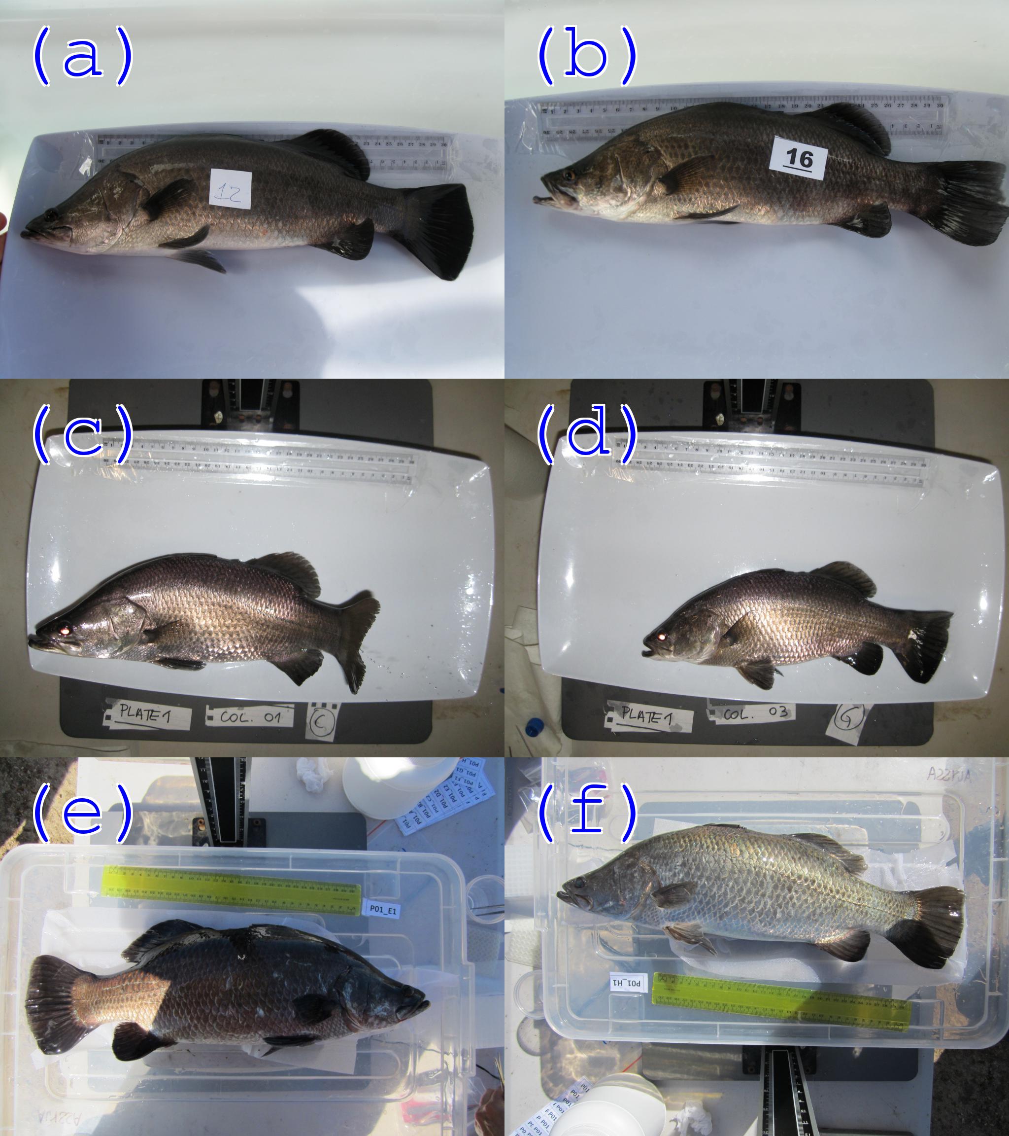
Figure 1: Samples of original images from the used datasets: BR445 (a) and (b), BW1400 (c) and (d), BA600 (e) and (f).

Figure 2: The same samples as in Fig. 1 converted to grayscale and enhanced by CLAHE [16].

The focus of this study was to continue developing methods for the automatic estimation of harvested fish weight from images. Specifically, the following practical and theoretical questions were addressed. Firstly, a practical application question: is it correct to assume (e.g. in [10]) that a model with excluded fins and tail would be more accurate compared to a model which used the whole fish silhouette? It is clearly much easier to extract the whole fish surface area than to exclude the non-exactly defined fins [6, 7]. Therefore, the additional complication of using the modern Deep Convolutional Neural Networks (CNNs) [10, 17] must be justified, for example, by a significantly more accurate mass-estimation model. The second practical question was to test how stable the Eqs. 5 and 6 models were when applied to a different set of barramundi images. From a theoretical point of view, the utilized (in [10]) semantic segmentation FCN-8s CNN [18, 19, 20] model was replaced here by the more recent LinkNet-34 [21, 22] CNN to test the stability and accuracy of the automatically segmented with-fins and without-fins fish surface areas.

The presented weight estimation pipeline was designed to be fast enough to process video frames as individual images in real time for the frame sizes up to $480\times 480$ resolution. In the aquaculture industry, a typical conveyor could be equipped with a video camera providing a video feed for the weight estimation processing. Furthermore, conveyor harvesting or transporting videos could be processed off-site, making the estimation procedure more financially viable and/or more accurate by processing the frames at higher resolutions. The required calibration could be easily achieved by sliding or placing a measuring ruler (or a known size object) on the conveyor. Note that for an actual industrial deployment it would be required to deal with tracking of individual fish and having multiple fish in the same frame, which was deemed outside the scope of this study.

II MATERIALS AND METHODS

II-A Datasets

Three datasets originated from [9] were used in this study. The Barra-Ruler-445 (BR445) dataset contained 445 images with manually measured weights in the range of $1-2.5$kg. BR445 was used in [10, 11, 12], see two typical examples in Figs. 1(a) and 1(b). The second dataset was Barra-Area-600 (BA600) containing more than 600 image-weight pairs (used in [10]), where BA600 fish weights were between 0.2 kg and 1 kg, see two examples in Figs. 1(e) and 1(f).

The third dataset (denoted BW1400) contained 1,400 harvested barramundi images with corresponding weight values from the $0.15-1.0$kg range. The BR445 and BA600 images were taken outdoors under the natural sunlight, while BW1400 images were taken indoors under artificial lighting. Note the same white holding plate (Figs 1a-d) had a blue tint in the BR445 images (Figs. 1a-b). To minimize dependency on such transient colors, in training and testing, all images were transformed to grayscale (Fig. 2).

II-B Semantic Segmentation of Images

The 200 no-fins masks from [10] together with the corresponding fish images were scaled to 1 mm-per-pixel, where 100 mask-image pairs were from BR445 and 100 from BA600, see examples in Fig. 3. In order to examine the fins/no-fins effect, additional 100 with-fins masks were manually segmented (50 from each BR445 and BA600), see example in Fig. 3(h). The lower number of the whole-fish masks (with fins) was justified by expecting the whole-fish segmentation to be a much easier problem to solve.

The most accurate Fully Convolutional Network from [18], FCN-8s, was trained on the 200 no-fins masks and applied in [10]. Even though FCN-8s was a major theoretical breakthrough when it was reported [18, 19], at the moment, FCN-8s is often less accurate than the more recent U-Net [20] type of segmentation CNNs. Furthermore, since only 200 no-fins masks out of the 1072 images in [10] were manually segmented, it was not possible to assess the actual accuracy of FCN-8s segmentations on the remaining not segmented images. Therefore, by using a different and more accurate (at least in theory) segmentation CNN in this study, we were aiming to assess the accuracy of the originally reported results obtained via FCN-8s.

A variation of U-Net [20], LinkNet-34 [21], was selected for this study, where ResNet-34 [23] was used as the feature encoder and the PyTorch implementation was from [22]. Two factors contributed to the choice of LinkNet-34. First, reproducibility of CNN results remains a challenge in many cases. This concern was mitigated by using the standard ResNet-34 CNN (available in the PyTorch distribution) together with the relatively simple LinkNet-34-style decoder, which was also available as an ”off-the-shelf” downloadable component [22]. The second deciding factor was that LinkNet-34 delivered a good balance of speed (verified during this project) and very high accuracy, which was demonstrated in the MICCAI 2017 Endoscopic Vision Sub-Challenge: Robotic Instrument Segmentation [24, 22].

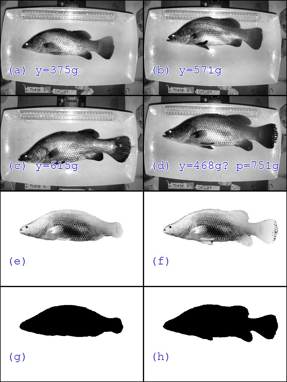
Figure 3: An example of weight measuring error in the BW1400 dataset: (a-c) the correctly measured reference images with $y$ weight values; (d) the identified recording/measuring error (predicted $p=751$g); (e) the mask without fins and tail for the fish in (d); (f) the whole fish mask for the fish in (d); (g) the mask without fins and tail; (h) the whole fish mask. Reversed grayscale was used in (e)-(h) for clarity.

II-C Training Pipeline

The training pipeline of [10] was retained as much as possible, where the following steps were similar or identical to [10]:

• The 200 no-fins masks and the 100 with-fins masks were split into training and validation sets as 80% and 20%, correspondingly.

• ResNet-34 layers were loaded with their ImageNet [25] trained weights to speed up the training process via the knowledge transfer [26]. The sigmoid activation function was used in the last output layer.

• Weight decay was set to $1\times 10^{-4}$ and applied to all trainable weights.

• All images and masks were scaled to 1 mm-per-pixel.

• To reduce overfitting for both training and validation, the image-mask pairs were randomly:

  • rotated in the range of $\pm 180$ degrees;

  • scaled in the range of [0.8, 1.2];

  • cropped to $480\times 480$ pixels;

  • flipped horizontally and/or vertically with 0.5 probability.

• Training was done in batches of 8 image-mask pairs.

• Adam [27] was used as a training optimizer.

Compared to [10], the following training steps were improved. As per [22], the loss function (Eq. 7) was replaced by (Eq. 8):

$$loss(y,\hat{y})=bc(y,\hat{y})+(1-dice(y,\hat{y}))$$ (7)

$$loss(y,\hat{y})=bc(y,\hat{y})-\ln(dice(y,\hat{y}))$$ (8)

where $y$ was a target mask, $\hat{y}$ was the corresponding LinkNet34 output, $bc(y,\hat{y})$ was the binary cross entropy, $dice(y,\hat{y})$ was the Dice coefficient [28]. For both training and testing, the input images were converted to one-channel gray images and normalized to the [0,1] range of numerical values. In order to reuse the ImageNet-trained ResNet-34 encoder, additional gray-to-color trainable conversion layer was added to the front of LinkNet-34 as per [29]. In addition to the original augmentations [10], image blurring (kernel sizes 3 or 5 pixels) or CLAHE [16] were applied with 0.5 probability each.

Use of LinkNet-34 as a more advanced segmentation CNN (compared to FCN-8s) together with grayscale images (and extensive augmentations) removed the necessity of freezing the ImageNet-trained encoder weights [10]. However, to assist in more effective re-use of the pre-trained ResNet-34, the Adam’s learning rate was reduced by factor of 10 when applied to the encoder (ResNet-34) layers. Adam’s starting learning rate ($lr$) was set to $lr=1\times 10^{-3}$ and then linearly reduced by 100 to $lr=1\times 10^{-5}$ over 100 training epochs. The blue line in Fig. 4 corresponds to the validation loss values while training over 100 epochs. With the same linear learning rate annealing schedule, if the same starting learning rate ($lr=1\times 10^{-3}$ or $lr=1\times 10^{-4}$) was applied to the ImageNet trained encoder (ResNet34) and the randomly initialized LinkNet34 decoder layers, the validation loss decreased less rapidly compared to our approach, see Fig. 4. If not frozen, lower learning rate was needed [30] for the ImageNet trained layers (e.g. ResNet-34 encoder) not to be randomized while training together with randomly initialized layers (e.g. LinkNet-34 decoder layers).

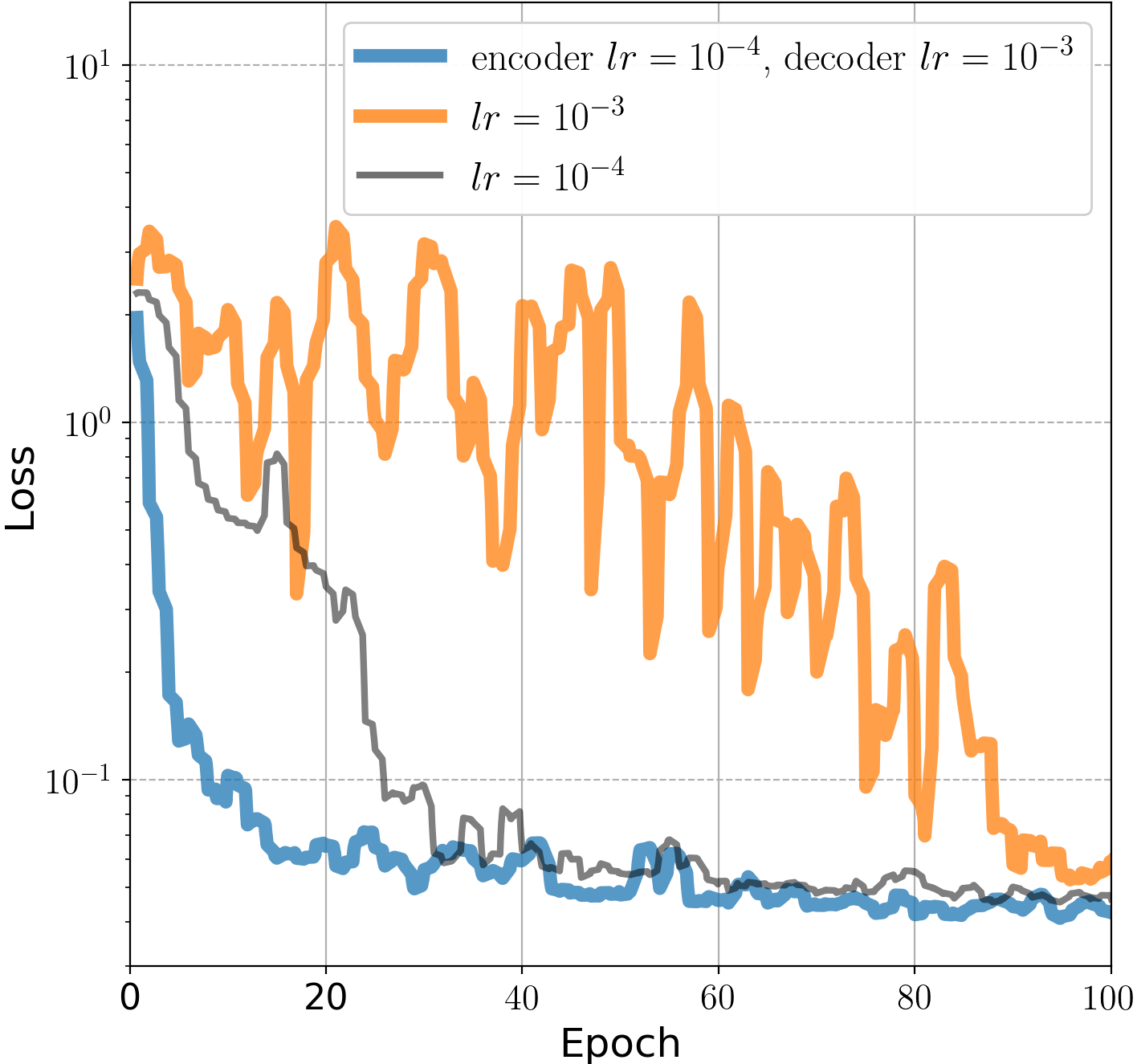
Figure 4: Effect of learning rates on validation losses

III Results and Discussion

The main goal of this study was to continue developing the best practice approaches to automatic estimation of the weight of harvested fish from images. This goal was approached via weight-from-area and weight-from-image models.

III-A Weight-from-area mathematical models

The first step was to examine whether the simple mathematical models estimating fish mass $M$ from its image surface area $S$, see Eqs. 5 and 6, were accurate and reliable for the industry. This approach was a simple (to understand and explain) way of any object weight estimation from its image surface area.

III-A1 With or without fins

We examined two mathematical models, see Eqs. 5 and 6, if they were more accurate by using only the fish body (the “no-fins“ rows of Table I) rather than the whole fish including fins and tail (the “whole” rows in Table I). The results in rows 1 and 2 (cells highlighted blue) revealed that for the one-factor model (Eq. 5), the coefficient of determination ($R^{2}$) and the mean absolute percentage error (MAPE) were indeed better for the no-fins models. Similar, the two-factor model (Eq. 6) was more accurate for the no-fins automatically segmented masks (cells highlighted orange). Here only the fitting performance of the models was considered, where the predictive accuracy was discussed in due course below.

TABLE I: Mass estimation models

Mask	Model	Fit	Fit	BW1400
type	Fitted or trained on	$R^{2}$	MAPE	MAPE
	BR445 and BA600		[%]	[%]
1. whole	$c=0.1254$	0.976	5.44	4.36
2. no-fins	$c=0.1718$	0.979	5.32	6.75
	Eq. 5, log-MSE fit
3. no-fins	$c=0.1702$	0.983	5.58	7.57
	Eq. 5, MSE fit [10]
4. whole	$a=0.0837$, $b=1.567$	0.979	4.68	6.19
5. no-fins	$a=0.1099$, $b=1.577$	0.982	4.33	10.35
	Eq. 6, log-RANSAC fit
6. no-fins	$a=0.1239$, $b=1.550$	0.983	4.53	11.51
	Eq. 6, MSE fit [10]
7. whole	LinkNet-34R		4.27	11.4
8. no-fins	LinkNet-34R		4.20	4.28

III-A2 Linear fit in logarithmic scale

Furthermore, the original fit (row 3 of Table I) was not done in logarithmic scale and therefore larger weights had disproportionately larger contribution to the fit (compare top and bottom rows in Fig. 5), which was done by minimizing the mean squared error (MSE). In this study, rows 1 and 2 were fitted (still by minimizing MSE) in logarithmic scale [7] (top row in Fig. 5) thus improving the MAPE from 5.58% to 5.32% (rows 2 and 3 of Table I). The MAPE improvement (due to the exclusion of fins and tail) was less pronounced if the MSE fitting was done directly on the area and weight values, not their logarithms. Fig. 5 illustrates how qualitatively similar the without-fins (left sub-figures) and with-fins (right sub-figures) distributions were, where higher density of data points was drawn by a lighter (yellow) color. Fig. 5 suggested a possible explanation of why some previous studies did not detect the improvement from the no-fins masks [6].

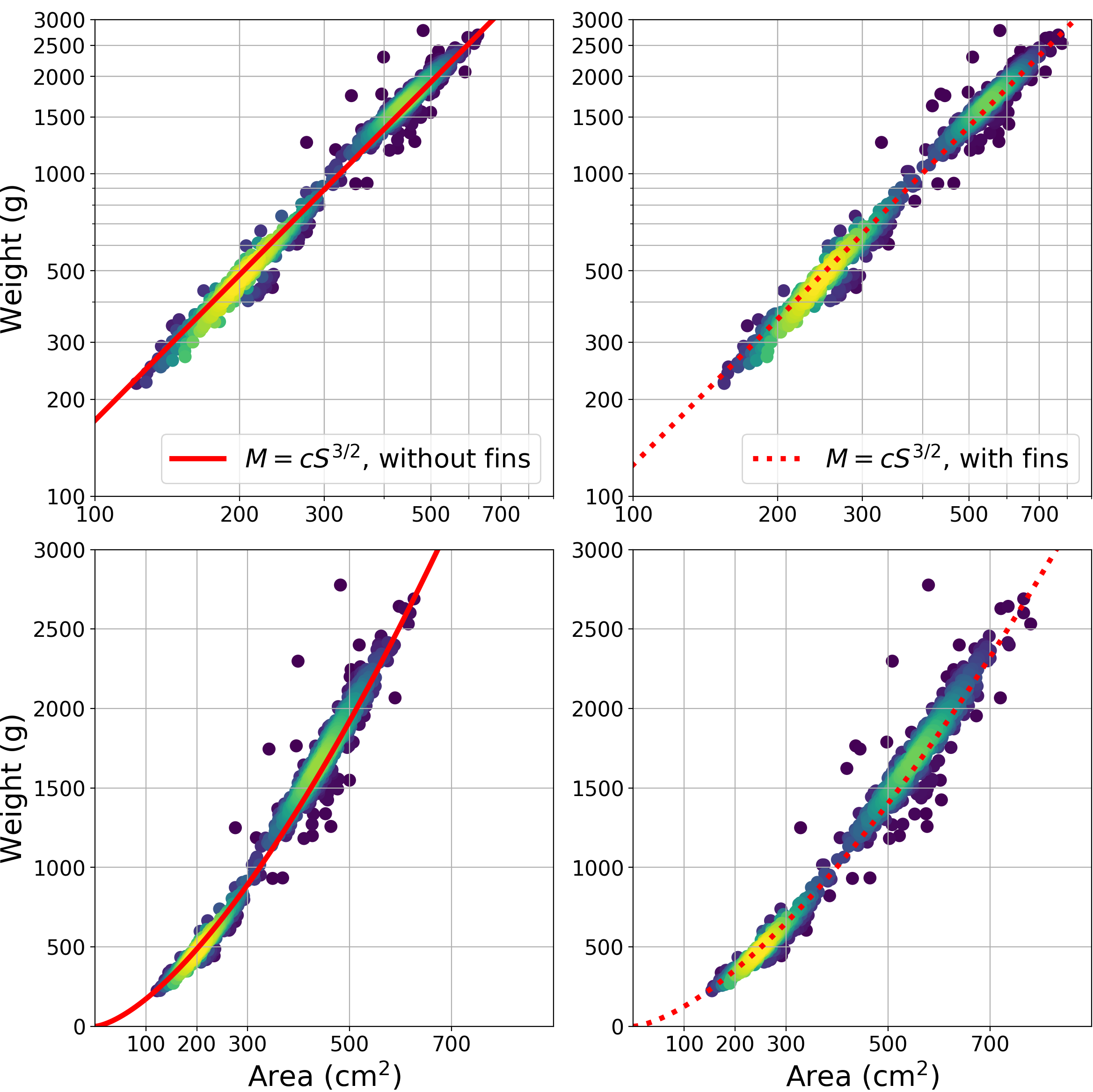
Figure 5: Relation between the measured fish weight and the automatically segmented fish area for the combined BR445 and BA600 datasets: without fins and tail (left figures), the whole fish (right figures).

III-A3 Outliers and robust fit

Fig. 5 also exposed a number of outliers. One approach dealing with the possible outliers was to use robust linear regression [31], which was adopted in this work by fitting the two-factor model (Eq. 6) via the RANSAC algorithm [32] in the logarithmic scale (top row of Fig. 5), see rows 4 and 5 in Table I. The two-factor fitting coefficient $b$ was different by less than 1% between the with-fins ($b=1.567$) and no-fins ($b=1.577$) models indirectly confirming that the RANSAC fit was indeed robust to the outliers. As expected, the robust fit of automatically segmented fish silhouettes without fins and tails achieved the best $\mbox{MAPE}=4.33\%$ of all considered mathematical models.

III-A4 Image collection procedure

Similar to the one-factor model, an improvement of about 0.35% was observed in the no-fins $\mbox{MAPE}=4.33\%$, see Table I cells highlighted orange. However, the image scales were accurate to approximately 1-2%, where the scales were taken from the rulers present in every image. The visual distortion of the ruler often yielded up to 1% different number of pixels between the top and bottom graduation markings (per ruler length). Therefore, in practical sense, a better image collection procedure could be more important than excluding fins and tail for the model building purposes.

III-B Weight-from-image estimation

In the preceding sections, a fish image was segmented into the background zero-values pixels and the value-of-one fish-mask with or without fins via the LinkNet-34 segmentation CNN. The threshold of accepting the LinkNet-34 sigmoid output as one (foreground pixels) was not fine-tuned and was left at its default 0.5 value. Then the total number of nonzero pixels were added to obtain the fish area $S$, which was fitted to the corresponding fish weight $M$ via Eqs. 5 or 6. Effectively, every foreground fish pixel was assumed to contribute equally to the total fish mass. While the simple mathematical models were easy to interpret, Standley et al. [33], in 2017, reported one of the first applications of CNNs for image-to-mass conversion achieving $\mbox{MAPE}<1\%$ on more than 1,300 test images of generic everyday-life and household objects, where the training collection had around 150,000 images. Hence, it was interesting to explore the direct conversion of the segmented mask to weight via the regression version of LinkNet-34, denoted LinkNet-34R.

The LinkNet-34R was obtained from LinkNet-34 by adding up all the LinkNet-34 sigmoid outputs without thresholding and converting the sum $y_{s}$ to the logarithmic scale:

$$y_{r}=log(y_{s}+1),$$ (9)

where 1 was added to assign a zero mass value to images without detected fish foreground masks. The automatically segmented fish images (not just masks), see examples in Fig. 3(e) and  3(f), were used as inputs to LinkNet-34R to make sure that predicted weight values from the CNN outputs were correlated to the fish image (with or without fins) versions and not anything else. The corresponding training fish weights were log scaled via the same Eq. 9 by replacing $y_{s}$ with the $M$ weight values. The LinkNet-34R training pipeline remained identical to that of LinkNet-34 with the only difference of not randomly rescaling the images, while the random scaling within 80%-120% range was used for LinkNet-34 but not for LinkNet-34R. Since the LinkNet-34 was already trained to detect the fish correctly, the LinkNet-34R version was loaded with the LinkNet-34 parameters and then trained starting from the learning rates reduced by factor of 10 in fine-tuning regime.

While running numerical experiments, large errors were examined and in approximately 1-2% of all image-weight pairs some image and/or recording/measuring errors were identified. For example, comparing identically scaled (1 mm-per-pixel) images in Fig. 3(a)-(d), the expected weight of the (d) case should be more that 615g and was predicted as 751g, while due to record-taking or measuring error it was recorded as 468g. Such obvious errors were removed from the BW1400 dataset but not from the BR445 and BA600 datasets, so that the results of this study could be directly compared to those of [10]. As per the image2mass study [33] and since quite a few outliers remained in the BR445 and BA600 datasets (Fig. 5), Mean Absolute Error (MAE) metric was used as the loss function when training the regression LinkNet-34R model. Using MSE would have resulted in fitting the outliers [31]. All 1,072 available BR445 and BA600 segmented image-weight pairs were randomly split into 80% and 20% for training and validation subsets, respectively, and the training subset was used to train the LinkNet-34R models. The validation (not training) MAPE values (4.27% and 4.20%) were reported in rows 7 and 8 of Table I.

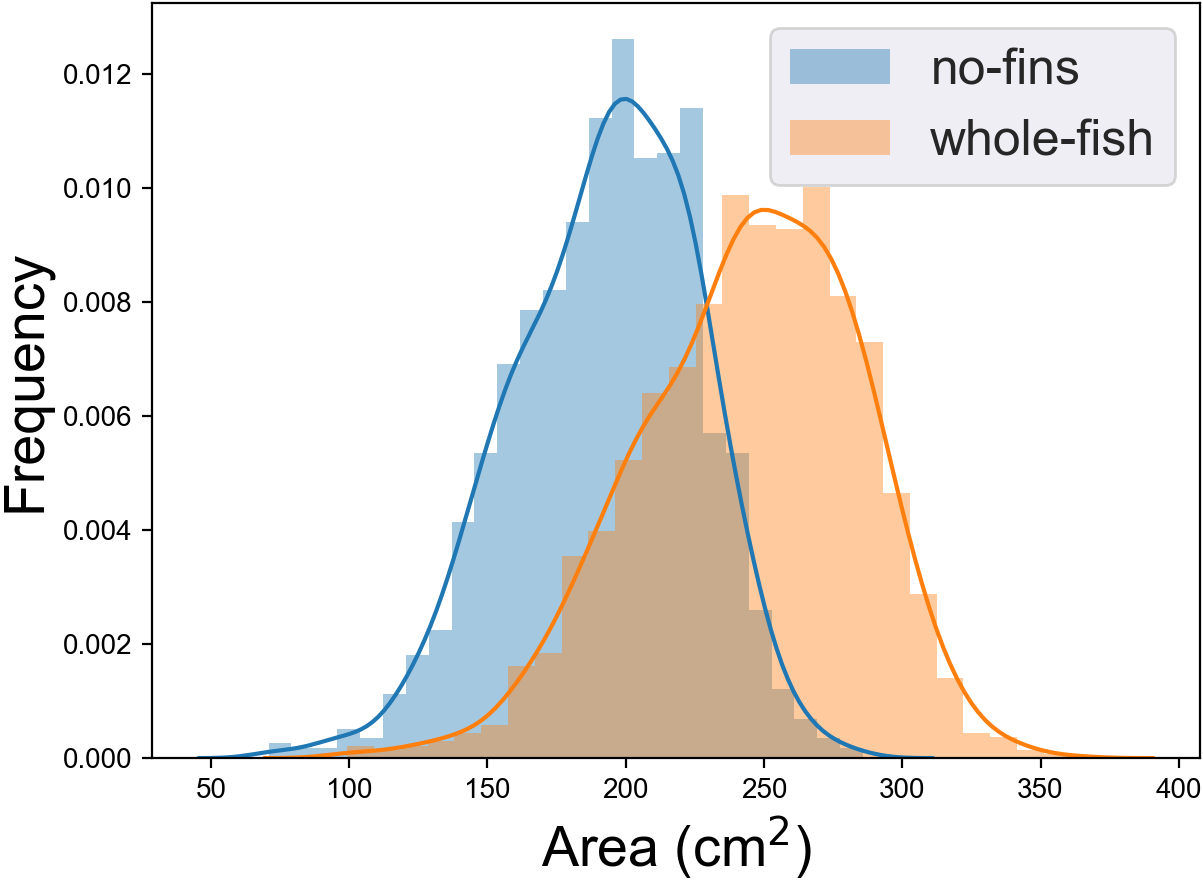
Figure 6: Normalized distributions of automatically segmented mask areas in the BW1400 images.

III-C Predictive performance of the models

As such, fitting known fish weights via a mathematical model or a neural network has little practical value unless the models could predict fish weights from new fish images. The last column of Table I examined the predictive accuracy of the models, which were fitted on BR445 and BA600 and then applied to the new BW1400 dataset. In practical industrial applications, the theoretical metrics such as $R^{2}$ becomes largely irrelevant, hence only MAPE was discussed hereafter. Our interpretation of the somewhat contradictory MAPE values were as follows.

III-C1 Whole-fish mathematical models predicted better

In row 1 of Table I, it was unrealistic to accept that the test $\mbox{MAPE}=4.36\%$ was indeed better than the fitting $\mbox{MAPE}=5.44\%$. Nevertheless, both the one- and two-factor whole-fish models achieved significantly better MAPE values (4.36% and 6.19%) for the unseen BW1400 images, compared to the corresponding no-fins models (6.75% and 10.35%). This was consistent with the no-fins models from [10], rows 3 and 6 in Table I, when applied to the new data.

III-C2 Errors in no-fins masks had larger effect

Trying to understand why the whole-fish models predicted better, it was noticed that very often the lower-front (pelvic) fins overlapped the body and were segmented out by the no-fins CNN, see examples in Figs. 2(c), 2(d) and 3(b). On average, the no-fins mask areas were 20% smaller than the corresponding whole-fish areas, see Fig. 6. Therefore, the erroneous reductions of no-fins masks (e.g. due to the overlapping pelvic fins) had larger weight error contributions than the variations of the fins in the whole-fish masks.

III-C3 Two-factor models overfitted and one-factor models predicted better

Further insight was gained by observing how the one-factor models (4.36% and 6.75% MAPEs, rows 1 and 2 in Table I) performed much better than the corresponding two-factor models (6.19% and 10.35% MAPEs, row 4 and 5). Therefore, the better fitting performance of the two-factor models (4.48% and 4.33%, rows 4 and 5) was most likely just the overfitting of the training datasets, which was consistent with the one-factor model remained more stable when refitted on all available BR445 and BA600 samples in [10].

III-C4 Direct weight-from-image CNN regression

The simple mathematical models (Eqs. 5 and 6) were based on the hypothesis that each fish pixel contributed equally to the total fish weight. The preceding results indicated that the hypothesis could be a very crude approximation, which did not perform well beyond the one-factor models. By forgoing the easy interpretability of the Eqs. 5 and 6, the LinkNet-34R CNN models performed highly non-linear conversion of the segmented fish images to weights. The no-fins version achieved nearly identical validation $\mbox{MAPE}=4.20\%$ and test $\mbox{MAPE}=4.28\%$, see row 8 in Table I. However, the whole-fish version exhibited some overfitting similar to the two-factor model: validation $\mbox{MAPE}=4.27\%$ but test $\mbox{MAPE}=11.4\%$ (row 7 in Table I).

Detailed investigation of how the CNNs arrived at the weight predictions was left for future work. In this study, we could only suggest the following speculative explanation. The no-fins fish images, see example in Fig. 3(e), had smooth contour therefore LinkNet-34R had to use other features from within the fish images to calculate the weight. The whole-fish contours, see Fig. 3(f), were more complex and therefore were more likely to be memorized for the individual training images, and hence overfitted by the LinkNet-34R’s more than 21 million parameters.

IV Conclusion

Estimation of object mass from images is an emerging area of computer vision [33] with potentially high impact industrial applications. We demonstrated how a standard “off-the-shelf” segmentation CNN like LinkNet-34 from [22] could be trained efficiently using: (i) only 100-200 training image-mask pairs; (ii) a linear learning rate annealing schedule; and (iii) reduced learning rate for the ImageNet-trained encoder (ResNet-34). With- or without-fins fish masks were automatically segmented and fitted by simple mathematical models achieving 4-10% MAPE values (mean absolute percentage errors consistent with other studies, e.g. [3, 7]) on 1,400 test images not used in the fitting procedure and from different geographical location.

The first question of this study was to assess if a fish silhouette automatically segmented by the CNNs should or should not include fish fins and tail. Remarkably, the two simple mathematical models based on the whole-fish silhouette generalized better (lower MAPEs) when applied to the unseen test images from the different geographical location. The second main question was answered by demonstrating that the simplest one-factor (one-parameter) mathematical model performed better than the two-factor model on the new test images. Furthermore, the one-factor model was highly stable achieving a lower $\mbox{MAPE}=4.36\%$ on the test images than on the training images, $\mbox{MAPE}=5.44\%$.

We successfully tested a conversion of a segmentation CNN, LinkNet-34, to weight-predicting CNN, LinkNet-34R, achieving 4-11% test MAPE valuess. To the best of our knowledge, this study presents the first practical and easily reproducible weight-from-image approach, e.g. by downloading the LinkNet-34 CNN together with the corresponding training pipeline from [22] and then following the steps explained in this study. However, only the no-fins version of the direct regression via LinkNet-34R performed well on the test images strongly indicating possible overfitting of the whole-fish version.

References

- [1] H. Hong, X. Yang, Z. You, and F. Cheng, “Visual quality detection of aquatic products using machine vision,” Aquacultural Engineering, vol. 63, pp. 62–71, 2014.
- [2] J. M. Miranda and M. Romero, “A prototype to measure rainbow trout’s length using image processing,” Aquacultural engineering, vol. 76, pp. 41–49, 2017.
- [3] G. Sanchez-Torres, A. Ceballos-Arroyo, and S. Robles-Serrano, “Automatic measurement of fish weight and size by processing underwater hatchery images,” Engineering Letters, vol. 26, 2018.
- [4] B. Zion, A. Shklyar, and I. Karplus, “In-vivo fish sorting by computer vision,” Aquacultural Engineering, vol. 22, pp. 165–179, 2000.
- [5] M. Saberioon, A. Gholizadeh, P. Cisar, A. Pautsina, and J. Urban, “Application of machine vision systems in aquaculture with emphasis on fish: state-of-the-art and key issues,” Reviews in Aquaculture, vol. 9, pp. 369–387, 2017.
- [6] M. O. Balaban, M. Chombeau, D. Cırban, and B. Gümüş, “Prediction of the weight of alaskan pollock using image analysis,” Journal of food science, vol. 75, pp. E552–E556, 2010.
- [7] S. Viazzi, S. Van Hoestenberghe, B. Goddeeris, and D. Berckmans, “Automatic mass estimation of jade perch scortum barcoo by computer vision,” Aquacultural engineering, vol. 64, pp. 42–48, 2015.
- [8] K. Zenger, M. Khatkar, D. Jerry, and H. Raadsma, “The next wave in selective breeding: implementing genomic selection in aquaculture,” in Proc. Assoc. Advmt. Anim. Breed. Genet, vol. 22, 2017, pp. 105–112. [Online]. Available: https://bit.ly/2I5gV00
- [9] J. A. Domingos, C. Smith-Keune, and D. R. Jerry, “Fate of genetic diversity within and between generations and implications for dna parentage analysis in selective breeding of mass spawners: a case study of commercially farmed barramundi, lates calcarifer,” Aquaculture, vol. 424, pp. 174–182, 2014.
- [10] D. A. Konovalov, A. Saleh, J. A. Domingos, R. D. White, and D. R. Jerry, “Estimating mass of harvested asian seabass lates calcarifer from images,” World Journal of Engineering and Technology, vol. 6, p. 15, 2018.
- [11] D. Konovalov, J. Domingos, R. White, and D. Jerry, “Automatic scaling of fish images,” in Proceedings of the 2nd International Conference on Advances in Image Processing. ACM, 2018, pp. 48–53.
- [12] D. Konovalov, J. Domingos, C. Bajema, R. White, and D. Jerry, “Ruler detection for automatic scaling of fish images,” in Proceedings of the International Conference on Advances in Image Processing. ACM, 2017, pp. 90–95.
- [13] G. G. Monkman, K. Hyder, M. J. Kaiserc, and F. P. Vidal, “Using machine vision to estimate fish length from images using regional convolutional neural networks,” Methods in Ecology and Evolution, p. in press, 2019.
- [14] J. S. Huxley, “Constant differential growth-ratios and their significance,” Nature, vol. 114, pp. 895–896, 1924.
- [15] B. Zion, “The use of computer vision technologies in aquaculture – a review,” Computers and Electronics in Agriculture, vol. 88, pp. 125 – 132, 2012.
- [16] K. Zuiderveld, “Contrast limited adaptive histogram equalization,” in Graphics gems IV. Academic Press Professional, Inc., 1994, pp. 474–485.
- [17] Y. LeCun, Y. Bengio, and G. Hinton, “Deep learning,” nature, vol. 521, p. 436, 2015.
- [18] E. Shelhamer, J. Long, and T. Darrell, “Fully convolutional networks for semantic segmentation,” IEEE Transactions on Pattern Analysis and Machine Intelligence, vol. 39, pp. 640–651, 2017.
- [19] J. Long, E. Shelhamer, and T. Darrell, “Fully convolutional networks for semantic segmentation,” in Proceedings of the IEEE conference on computer vision and pattern recognition, 2015, pp. 3431–3440.
- [20] O. Ronneberger, P. Fischer, and T. Brox, “U-net: Convolutional networks for biomedical image segmentation,” in International Conference on Medical image computing and computer-assisted intervention. Springer, 2015, pp. 234–241.
- [21] A. Chaurasia and E. Culurciello, “Linknet: Exploiting encoder representations for efficient semantic segmentation,” in 2017 IEEE Visual Communications and Image Processing (VCIP). IEEE, 2017, pp. 1–4.
- [22] A. A. Shvets, A. Rakhlin, A. A. Kalinin, and V. I. Iglovikov, “Automatic instrument segmentation in robot-assisted surgery using deep learning,” in 2018 17th IEEE International Conference on Machine Learning and Applications (ICMLA). IEEE, 2018, pp. 624–628.
- [23] K. He, X. Zhang, S. Ren, and J. Sun, “Deep residual learning for image recognition,” in Proceedings of the IEEE conference on computer vision and pattern recognition, 2016, pp. 770–778.
- [24] “MICCAI 2017 endoscopic vision challenge: Robotic instrument segmentation sub-challenge,” 2017. [Online]. Available: https://bit.ly/2jZ9Ia3
- [25] O. Russakovsky, J. Deng, H. Su, J. Krause, S. Satheesh, S. Ma, Z. Huang, A. Karpathy, A. Khosla, M. Bernstein et al., “Imagenet large scale visual recognition challenge,” International journal of computer vision, vol. 115, pp. 211–252, 2015.
- [26] M. Oquab, L. Bottou, I. Laptev, and J. Sivic, “Learning and transferring mid-level image representations using convolutional neural networks,” in Proceedings of the IEEE conference on computer vision and pattern recognition, 2014, pp. 1717–1724.
- [27] D. P. Kingma and J. Ba, “Adam: A method for stochastic optimization,” in ICLR, 2015.
- [28] L. R. Dice, “Measures of the amount of ecologic association between species,” Ecology, vol. 26, pp. 297–302, 1945.
- [29] D. A. Konovalov, S. Jahangard, and L. Schwarzkopf, “In situ cane toad recognition,” in 2018 Digital Image Computing: Techniques and Applications (DICTA). IEEE, 2018, pp. 1–7.
- [30] J. Howard, R. Thomas, and S. Gugger, “FastAI,” 2019. [Online]. Available: https://www.fast.ai
- [31] D. A. Konovalov, L. E. Llewellyn, Y. Vander Heyden, and D. Coomans, “Robust cross-validation of linear regression QSAR models,” Journal of Chemical Information and Modeling, vol. 48, pp. 2081–2094, 2008.
- [32] M. A. Fischler and R. C. Bolles, “Random sample consensus: A paradigm for model fitting with applications to image analysis and automated cartography,” Commun. ACM, vol. 24, pp. 381–395, 1981.
- [33] T. Standley, O. Sener, D. Chen, and S. Savarese, “image2mass: Estimating the mass of an object from its image,” in Conference on Robot Learning, 2017, pp. 324–333.