TESS observations of the WASP-121 b phase curve

Abstract

We study the red-optical photometry of the ultra-hot Jupiter WASP-121 b as observed by the Transiting Exoplanet Survey Satellite (TESS) and model its atmosphere through a radiative transfer simulation. Given its short orbital period of $\sim 1.275$ days, inflated state and bright host star, WASP-121 b is exceptionally favorable for detailed atmospheric characterization. Towards this purpose, we use allesfitter to characterize its full red-optical phase curve, including the planetary phase modulation and the secondary eclipse. We measure the day and nightside brightness temperatures in the TESS passband as $3012\begin{subarray}{c}+40\\ -42\end{subarray}$ K and $2022\begin{subarray}{c}+254\\ -602\end{subarray}$ K, respectively, and do not find a statistically significant phase shift between the brightest and substellar points. This is consistent with an inefficient heat recirculation on the planet. We then perform an atmospheric retrieval analysis to infer the dayside atmospheric properties of WASP-121 b such as its bulk composition, albedo and heat recirculation. We confirm the temperature inversion in the atmosphere and suggest H^-, TiO and VO as potential causes of the inversion, absorbing heat at optical wavelengths at low pressures. Future HST and JWST observations of WASP-121 b will benefit from its first full phase curve measured by TESS.

1 Introduction

A planet’s occultation as it passes behind its host star, i.e., the secondary eclipse, reveals atmospheric characteristics such as the dayside temperature and reflectivity (Agol et al., 2010; Line et al., 2013). Furthermore, changes in the brightness of a planet and star system as a function of orbital phase (i.e., the phase curve), contain information about the dynamics of the orbit as well as the thermal state on the nightside and heat recirculation on the planet (Cowan & Agol, 2008; Angerhausen et al., 2015; Shporer, 2017; Zhang et al., 2018; Shporer et al., 2019).

WASP-121 b is a transiting exoplanet with a period of $1.274928\pm 0.000011$ days discovered by Delrez et al. (2016). The host star WASP-121 has the TESS Input Catalog (TIC) number 22529346 and is a F6V type star with radius of $1.52\pm 0.06$ R_⊙, mass of $1.45\pm 0.25$ M_⊙, and effective temperature of $6776\pm 134$ K (Stassun et al., 2019). WASP-121 b belongs to a class of exoplanets known as ultra-hot Jupiters that orbit their host stars with short ($\sim 1$ day) periods and have dayside temperatures larger than 2200 K. Given its short orbital period, it is likely that WASP-121 b is locked to its host star via tidal interactions. Furthermore, WASP-121 b has various features that make it an exceptional exoplanet. First, its short orbital period and hot host star cause it to be highly irradiated, raising its dayside near-infrared brightness temperature to $\sim$2700 K (Evans et al., 2017). Second, it has a spin-orbit angle of $258^{\circ}\pm{5^{\circ}}$ (Delrez et al., 2016), indicating that the planet’s orbit is nearly anti-aligned with the stellar spin axis. Third, given its mass and radius of $\sim$1.2 and $\sim$1.9 times that of Jupiter (Delrez et al., 2016), respectively, WASP-121 b is an inflated exoplanet that nearly fills its Roche lobe. This means that it should be tidally disrupted and merge with its host star in the next few hundred million years. Furthermore, given its bright host star with a V magnitude of 10.5, aforementioned inflated state and availability of previously collected spectroscopic data, WASP-121 b is an interesting target for detailed atmospheric characterization. The James Webb Space Telescope (JWST) is expected to further characterize the atmosphere of WASP-121 b in the near and far-infrared via emission spectroscopy.

Previous work on WASP-121 b found evidence for emission and absorption features as opposed to a featureless blackbody spectrum (Mikal-Evans et al., 2020). In Evans et al. (2017), 1.4 $\mu$m infrared emission from hot H₂O molecules was detected in the emission spectrum of WASP-121 b using the Hubble Space Telescope (HST) Wide Field Camera 3 (WFC3) G102 grism. Along with the Spitzer measurements, this allowed atmospheric retrieval of WASP-121 b’s dayside. That the H₂O feature was observed in emission rather than absorption, is a potential indication that the upper layers of the atmosphere are hotter and that the temperature profile of the atmosphere is inverted. This requires the existence of a stratosphere (i.e., the layer of the atmosphere, where the temperature increases with altitude, which is significantly heated at low pressure). This temperature inversion can be realized by metal oxides such as Vanadium Oxide (VO) or Titanium Oxide (TiO) due to their strong absorption in the optical wavelengths. These molecules are commonly found in brown dwarfs and require high temperatures to be in gaseous form, such as that available on WASP-121 b. Moreover, an atmospheric transmission spectrum was observed using the Space Telescope Imaging Spectrograph (STIS) on HST, where evidence for VO was found (Evans et al., 2018). More recently, an emission spectrum for WASP-121 b in the 0.8–1.1 $\mu$m passband was collected using HST (Mikal-Evans et al., 2019). This provided evidence for the contribution of H^- to the optical opacity of WASP-121 b’s atmosphere. Furthermore in Sing et al. (2019) UV transmission spectroscopy was performed on WASP-121 b as part of the Panchromatic Comparative Exoplanet Treasury (PanCET) survey, revealing heavy ionized metals such as Mg and Fe in gas form, implying that they escape the planet instead of forming condensates.

In this work, we study the full phase curve of the WASP-121 system in the red-optical (i.e., 0.6–0.95 $\mu$m) passband as measured by the Transiting Exoplanet Survey Satellite (TESS; Ricker et al. 2014) in order to characterize the planetary modulation (i.e., thermal and reflected emission from the planet). We then discuss the implications of these measurements regarding the atmospheric properties of WASP-121 b, including optical reflectivity and heat recirculation.

The TESS data on WASP-121 b is important mainly for two reasons. First, TESS extends the wavelength coverage of the available data on the system by 0.2 $\mu$m towards shorter wavelengths as compared to the previously collected G102 data (Mikal-Evans et al., 2019). Interestingly, the TESS passband contains emission bands of TiO and VO, giving us a probe of their role in the temperature inversion. Second, the TESS data contain the full phase curve of the system, allowing inference of the nightside temperature as well as any phase shift between the bright spot (i.e., longitude of highest brightness) and the substellar point.

The rest of the paper is as follows. The data taken by TESS are presented in Section 2. Our methods of data analysis are presented in Section 3. We then present our results in Section 4 and end with a discussion and conclusion in Sections 5 and 6.

2 Data

The WASP-121 system was observed by the TESS mission at 2 minute cadence during Sector 7. The observations were carried out with camera 3 and the charge coupled device (CCD) 2, between 7 January 2019 and 2 February 2019, spanning orbits 21 and 22.

These short cadence target pixel files were analyzed by the Science Processing Operations Center (SPOC) pipeline (Jenkins et al., 2010, 2016; Smith et al., 2012; Stumpe et al., 2014) to produce simple aperture photometry (SAP) and presearch data conditioning (PDC) light curves. An alert was then issued by the TESS Objects of Interest (TOI) working group (TOI 495.01) based on the detected periodic transit signal.

In order to produce the SAP light curve, the SPOC pipeline subtracts a background photon count estimate from the total number of photons inside a given aperture, whereas the PDC data product also contains a correction for red noise as well as the decrease in the transit depth due to known nearby sources. These initial data are shown in the first (SAP) and second (PDC) panels of Figure 1, respectively. We inspected both data sets and concluded that the PDC light curve was not suitable for further analysis due to residual systematics in the data at short time scales, especially prominent in the second orbit of Sector 7. Red noise is mostly in the form of discontinuities and systematic trends introduced by instrumental effects such as changes in the thermal state of TESS and pointing instabilities. Therefore, we decided to fit a cubic spline to the SAP data collected during each individual orbit after masking out the flagged data points as well as the transits as shown in the third panel of Figure 1. This procedure filtered systematics introduced at a time scale much longer than the orbital period, while preserving the phase curve modulations.

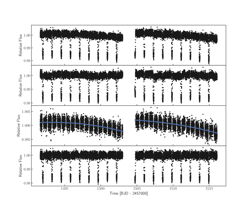
Figure 1: Top: the SAP TESS light curve of WASP-121. Second from the top: the PDC light curve of WASP-121, showing indications of excessive red noise. Third from the top: SAP light curve of WASP-121 after masking both the primary transits and the secondary eclipses of WASP-121 b (black) and the spline model (blue). Bottom: the detrended light curve on which the later analyses are based. In all panels, there is a gap in the middle of the data set due to TESS pausing data collection around perigee.

When fitting cubic splines, we increased the number of knots until the residual per degree of freedom fell below unity. The resulting coefficients and knot locations are given in Table 1 for each orbit separately. We then based the subsequent analyses on the detrended light curve obtained by removing the spline fit from the SAP light curve. The resulting detrended light curve is shown in the bottom panel of Figure 1. It is true that this leaves some red noise at short time scales in the resulting light curve, which can potentially bias our nominal fit. As a crosscheck, this detrended light curve was also modeled using a Gaussian Process (GP) in an alternative analysis, which will be described in Section 3.

	First orbit	Second orbit
$T_{i}$ [BJD]	2458491.63452417	2458503.0401359
$T_{f}$ [BJD]	2458504.83318593	2458516.08867022
$\beta_{0}$	0.00103486	1.91152409e-03
$\beta_{1}$	0.00140942	1.28100318e-03
$\beta_{2}$	0.00048103	-5.56292798e-05
$\beta_{3}$	-0.00212276	-2.75337528e-03

Table 1: Table of cubic spline coefficients, $\beta_{i}$ for $i~{}=~{}\{0,1,2,3\}$, for the first and second orbits, which begin and end at $T_{i}$ and $T_{f}$.

When extracting the light curve of a target, transits are diluted (i.e., their depths are decreased) due to light contamination from neighboring stars into the photometric aperture. Given the 21″pixel scale of TESS and the bright neighbors within $\sim$100″of WASP-121, WASP-121’s TESS light curve is expected to be diluted by $\sim$8.3%. However, the amount of dilution cannot be known precisely due to uncertainties in the point spread function. This results in an uncertainty that needs to be propagated forward during inference. Hence, in order to take into account the dilution of the transits in the (uncorrected) SAP light curves, we included a dilution parameter in the light curve model, imposing a Gaussian prior centered on the expected value of 8.3%.

The available data on WASP-121 b include: the secondary eclipse data at 3.6 $\mu$m and 4.5 $\mu$m collected by Spitzer (Garhart et al., 2019), $z^{\prime}$ photometry measured by TRAPPIST (Delrez et al., 2016), $K_{s}$ band photometry (Kovacs & Kovacs, 2019), G102 and G141 HST/WFC3 emission spectroscopy (Evans et al., 2017; Mikal-Evans et al., 2019); the transmission spectroscopy data collected during the primary transit from (Evans et al., 2018); and the TESS phase curve analyzed in this work. We utilize the secondary eclipse data to perform an atmospheric retrieval (see Section 3.3).

3 Methods

In this section, we lay out our methodology for modeling

1. the TESS light curve to infer the orbital properties and the phase curve characteristics of the WASP-121 system,

2. the resulting phase curve characteristics to infer the temperature distribution on WASP-121 b,

3. the multiband spectrum of WASP-121 b’s dayside to retrieve the atmospheric properties of the dayside of WASP-121 b.

3.1 Phase curve

The variation of the brightness of a star-exoplanet system during orbit, i.e., a phase curve, can be broken down into several components. First, the gravitational field of the star and the exoplanet tidally distorts the two bodies according to the Roche potential, causing ellipsoidal variations in the brightness of the system at a period equal to the half of the orbital period. Second, the radial velocity of the orbiting planet results in the redward and blueward shifting (i.e., Doppler boosting) of light from the star, at the orbital period. Lastly, the thermal and reflected emission from the planet change during an orbit, as a result of the changing fraction of the illuminated and heated surface of the planet. We will refer to the sum of the thermal and reflected emission from the planet as the planetary modulation component.

3.1.1 Ellipsoidal variation

Ellipsoidal variation is a measure of how the tidal gravitational field of the companion compares to the surface gravity of the host star. Its fractional amplitude can be expressed to leading order as (Morris, 1985; Morris & Naftilan, 1993)

$$D_{\rm e}=\alpha_{\rm e}\dfrac{M_{\rm p}}{M_{\star}}\sin^{2}i\Bigg{(}\dfrac{R_{\star}}{a}\Bigg{)}^{3},$$ (1)

where $\alpha_{\rm e}$ is a constant that depends on the linear limb darkening and gravity darkening coefficients, $M_{\rm p}$ and $M_{\star}$ are the mass of the planet and the star, $i$ is the orbital inclination, $R_{\star}$ is the radius of the star and $a$ is the semi-major axis.

We used the limb darkening and gravity darkening coefficients in Claret (2017) to predict the ellipsoidal variation amplitude of the WASP-121 system as $\sim$20 ppm, which justified the inclusion of ellipsoidal variations into our light curve model. Although strong ellipsoidal variations can manifest higher order terms (i.e., harmonics), we only included the first order (i.e., fundamental) term into the model and neglected higher order terms.

3.1.2 Doppler boosting

During the orbit of the companion, the line-of-sight velocity of the host star varies periodically, causing photons to be blue or red shifted. Therefore, although the bolometric flux does not change, the brightness of the host in a particular passband varies at the orbital period with the fractional amplitude of (Shporer, 2017)

$$D_{\rm b}=4\alpha_{\rm b}\frac{K}{c},$$ (2)

where

$$\alpha_{\rm b}=\int\frac{1}{4}\frac{xe^{x}}{e^{x}-1}dx,x\equiv\frac{hc}{kT\lambda}.$$ (3)

Here, $K$ is the radial velocity semi-amplitude, $c$ is the speed of light, $h$ is the Planck constant, $k$ is the Boltzmann constant, $T$ is the temperature of the star, and $\lambda$ is the wavelength. The integral is taken inside the TESS passband as shown in the top row of Figure 7. The Doppler boosting fractional amplitude we expect for this system was estimated as $\sim$1 ppm, which is much smaller than the uncertainties of the photometric data. Therefore, we did not include Doppler boosting in our light curve model.

3.1.3 Thermal and reflected planetary emission

As the planet orbits the host star, a changing fraction of its surface is illuminated. Therefore, both the reflected and thermal emission from the orbiting planet is expected to follow roughly a cosine at the orbital period whose maximum occurs near phase 0.5.

At the superior conjunction, the total secondary depth,

$$D_{\rm s}=D_{\rm t}+D_{\rm r},$$ (4)

can be generically expressed as the sum of a thermal, $D_{\rm t}$, and reflected, $D_{\rm r}$, components. Equation 4 shows that the thermal and reflected emissions are degenerate given some secondary eclipse data in a single band. Having spectral data, therefore, becomes crucial for placing an independent constraint on the thermal emission in order to break this degeneracy (Kreidberg et al., 2018; Mansfield et al., 2018).

The thermal component can further be written as (Charbonneau et al., 2005)

$$D_{\rm t}=\Bigg{(}\frac{R_{\rm p}}{R_{\star}}\Bigg{)}^{2}\times\dfrac{\int\mathcal{T}(\lambda)F_{\rm p}(\lambda,T_{\rm p})d\lambda}{\int\mathcal{T}(\lambda)F_{\star}(\lambda,T_{\star})d\lambda},$$ (5)

where $R_{\rm p}$ and $R_{\star}$ are the planetary and stellar radii, $\mathcal{T}$ is the TESS throughput and $F_{\rm p}(\lambda,T)$ and $F_{\star}(\lambda,T)$ are the planetary and stellar fluxes, which are roughly blackbodies with effective temperatures $T_{\rm p}$ and $T_{\star}$. The reflected component, on the other hand, is given by (Rodler et al., 2010)

$$D_{\rm r}=A_{\rm g}\Bigg{(}\frac{R_{\rm p}}{a}\Bigg{)}^{2},$$ (6)

where $A_{\rm g}$ is the geometric albedo in the TESS passband, which quantifies the reflectivity of a planet relative to that of a Lambertian disk and differs from the Bond albedo, $A_{\rm B}$, which is the ratio of the reflected bolometric flux to that received from the host star.

The brightness of an ultra-hot Jupiter in the infrared is dominated by its thermal emission. However, it may get an increasing contribution from reflection at shorter wavelengths, such as those probed by TESS. Reflection of incident light causes the equivalent temperature of the planet to be reduced at fixed stellar radius and orbital semi-major axis. Another process with which the dayside equivalent temperature of a planet can be reduced is heat recirculation from the dayside to the nightside, which can partially homogenize the temperature distribution across the exoplanet.

3.1.4 Light curve model

We modeled the TESS light curve using allesfitter (Günther & Daylan, 2019; Guenther & Daylan, 2020). Given the orbital phase between 0 and 1, $\phi$, we assume the primary transit and secondary eclipse to happen at phases 0 and 0.5, respectively. The resulting light curve model can be expressed as a linear combination of the following components:

• Baseline stellar emission. This component assumes a constant stellar emission, which is partially occulted during the primary transit of the planet according to our transit model (calculated via ellc),

• Constant planetary emission. This component models the planet as a constant source of emission. It is parametrized by the surface brightness ratio of the planet and the star, $J$, outside the secondary eclipse and is 0 otherwise (calculated via ellc).

• Planetary modulation. The modulation has the form of $D_{\rm p}(1-\cos 2\pi(\phi+\Delta_{\rm p}/P))/2$ outside the secondary eclipse and is 0 otherwise. Here, $P$ is the orbital period and $\Delta_{\rm p}$ allows us to model a nonzero phase shift.

• Ellipsoidal variation. The ellipsoidal variation is modeled as $D_{\rm e}(1-\cos 4\pi\phi)/2$, i.e., a sinusoidal at half of the orbital period that peaks at quadrature (0.25 and 0.75) phases.

• A constant offset to absorb any normalization bias denoted by $O$.

We model the baseline stellar emission, primary transit, and the secondary eclipse in terms of the following parameters: the planet-to-star radius ratio, $R_{\rm p}/R_{\star}$; the ratio of the sum of the stellar and planetary radius and the semi-major axis of the orbit, $(R_{\star}+R_{\rm p})/a$; the cosine of the orbital inclination, $\cos i$; the epoch, $T_{0}$; the period, $P$; the terms parametrizing the orbital eccentricity, $\sqrt{e}\cos\omega$ and $\sqrt{e}\sin\omega$, where $e$ and $\omega$ are the eccentricity and argument of periapsis; the dilution in the TESS frames, $D_{\rm TESS}$; transformed limb darkening coefficients $q_{1}$ and $q_{2}$; the logarithm of the average measurement uncertainty of the relative flux data, $\log\sigma$; and a flat baseline fitted to the light curve, $O$. We assume zero eccentricity Delrez et al. (2016). As for limb darkening, we use the transformed set of limb darkening coefficients, $q_{1}\equiv(u_{1}+u_{2})^{2}$ and $q_{2}\equiv 0.5(u_{1}+u_{2})^{-1}$ (Kipping, 2013), which allows us to efficiently sample from the posterior of the limb darkening coefficients. When fitting the relative flux data, we allow a free rescaling of the uncertainties, where we first normalize the measurement uncertainties of relative flux by dividing them by the mean uncertainty and then multiplying these normalized uncertainties by $\sigma$ defined above.

The main challenge in modeling data with systematic errors is red noise, which is the result of all instrumental and astrophysical processes that are not available in the forward-model used to fit a given data set. Thanks to their flexibility, GPs can be used to model red noise. In particular, allesfitter has a built-in GP with the Matérn 3/2 kernel with the hyperparameters $\sigma_{\rm GP}$ (amplitude) and $\rho_{\rm GP}$ (time scale). In this work, our nominal fit employs a light curve model with a flat baseline. However, as a crosscheck to our nominal fit, we performed an additional fit using a GP as the baseline model.

We note that the TESS data, being bluer than other available secondary eclipse data on the system, probe relatively higher altitudes in the atmosphere, and thus has more constraining power on the temperature inversion. It is also the case that, being bluer than other passbands, the TESS data are more susceptible to stellar variability. Our light curve model with the GP can absorb any stellar variability. Therefore, this alternative fit also brackets the range of solutions consistent with the TESS data, marginalizing over stellar variability.

Given the above-mentioned forward model and the spline-detrended TESS light curve, we sample from the posterior distribution subject to certain priors using emcee (Foreman-Mackey et al., 2013). In order to make sure that the samples taken from the posterior are fair and that the chains are converged, we collect samples until the chain length is at least 30 times that of the integrated autocorrelation time of all parameters. The definition of our parameters, the priors imposed, and the posterior are listed in Table 2.

3.2 Temperature distribution

In the absence of any heat circulation, the equilibrium temperature of the planet, $T_{\rm eq}$, is given by

$$T_{\rm eq}=T_{\star}(1-A_{\rm B})^{1/4}\sqrt{\dfrac{R_{\star}}{2a}}$$ (7)

where $T_{\star}$ is the effective temperature of the host star, $a$ is the orbital semi-major axis, $E$ is the planetary emissivity and $A_{\rm B}$ is the Bond albedo. Furthermore, when there is heat recirculation between the day and night sides of a planet, the dayside and the nightside temperatures, $T_{\rm d}$ and $T_{\rm n}$, can be parametrized as,

$$T_{\rm d} =T_{\rm eq}\Big{(}\frac{2}{3}-\frac{5}{12}\varepsilon\Big{)}^{1/4}\equiv\psi T_{d,0},$$ (8)

$$T_{\rm n} =T_{\rm eq}\Big{(}\frac{\varepsilon}{4}\Big{)}^{1/4},$$ (9)

respectively, where $\varepsilon$ parametrizes the heat recirculation efficiency (Cowan & Agol, 2011). An $\varepsilon$ of 0 indicates no heat recirculation whereas an $\varepsilon$ of 1 implies instantaneous redistribution of incident energy over the planet. Here, the dayside temperature in the case of perfect emissivity and the absence of any heat recirculation, reflection and internal heat is denoted by $T_{d,0}$. Therefore $\psi$ is a parameter that takes into account the effect of any reflection, heat recirculation and planetary internal heat. In particular, $\psi$ is equal to 1 when there is no heat recirculation, the planet does not reflect any light, and in the limit of zero internal heat.

In the absence of any heat recirculation, the point on the surface of a tidally-locked planet directly pointing to the host star, i.e., the substellar point, is expected to be the hottest point on the surface of the planet (Mazeh, 2008). However, heat recirculation in the atmosphere (e.g., via winds due to atmospheric pressure gradients) can transport energy and result in an eastward phase shift. Another potential source of phase shift is reflective clouds on the western hemisphere. Although the dayside temperature of ultra-hot Jupiters is typically too high for reflective condensates to be sustained, refractory species can still form on the nightside of the planet. Furthermore, the western terminator of a hot Jupiter is expected to be colder than the eastern one, because the super-rotating equatorial jet moves cold gas from the nightside to the western terminator of the planet. When this gas is sufficiently cool, condensates can remain stable on the western terminator. This can result in some reflected light from the western limb and cause a westward phase shift (Parmentier et al., 2016). Therefore, there can be distinct phase shifts for the thermal and reflected emissions.

In our nominal fit, we use a light curve model with a single planetary modulation component with amplitude $D_{\rm p}$ and phase shift $\Delta_{\rm p}$. This effectively accounts for the sum of the reflected and thermal components, which are largely degenerate. We do, however, perform an alternative fit, where we use two different planetary modulation components with amplitudes $D_{\rm 1}$ and $D_{\rm 2}$ and phase shifts $\Delta_{\rm 1}$ and $\Delta_{\rm 2}$. Nevertheless, we present this fit only as a crosscheck, as it potentially overfits the data, since the two components are largely degenerate.

Given an estimate of the thermal phase shift and the dayside and nightside temperatures of a planet, one can also parametrically infer the temperature distribution. Towards this purpose, we solve the kinematic differential equation (Zhang & Showman, 2017)

$$\frac{\partial T}{\partial t}+\frac{1}{\tau_{adv}}\frac{\partial T}{\partial\lambda}=\frac{1}{\tau_{rad}}(T_{eq}(\lambda)-T)$$ (10)

which describes the heat recirculation, and hence, the temperature distribution on the planet, where $T$ is the effective temperature, $\lambda$ is the longitude, $\tau_{adv}$ and $\tau_{rad}$ are the advective and radiative time scales, respectively. Their ratio, $\xi\equiv\tau_{rad}/\tau_{adv}$, is related to, but distinct from the heat recirculation efficiency $\varepsilon$ defined previously. Although they are both zero in the limit of vanishing heat recirculation, the limit $\xi\to\infty$ corresponds to $\varepsilon$ $\sim$0.95. At constant longitude, we assume that the temperature on the planet is proportional to $\cos(\theta)$ as a function latitude, $\theta$. The solution of Equation 10 yields the form

$$T(\lambda)=\begin{cases}T_{\rm n}+T_{1}\cos\lambda_{s}\cos(\lambda-\lambda_{s})+\eta T_{1}e^{-\lambda/\xi}\\ \hskip 60.00009pt\text{ for $-\pi/2<\lambda<\pi/2$}\\ T_{\rm n}+\eta T_{1}e^{-(\pi+\lambda)/\xi}\text{ for }-\pi<\lambda<-\pi/2\\ T_{\rm n}+\eta T_{1}e^{(\pi-\lambda)/\xi}\text{ for }\pi/2<\lambda<\pi,\end{cases}$$ (11)

where $T_{1}$ is the temperature difference between the anti-stellar and sub-stellar points on the planet, $T_{\rm n}$ is the temperature of the nightside, and $\eta$ and $\lambda_{s}$ are defined as

$$\eta=\frac{\xi}{1+\xi^{2}}\frac{1}{e^{\pi/2\xi}-1}\Bigg{(}e^{\frac{\pi}{2\xi}}+e^{\frac{3\pi}{2\xi}}\Bigg{)}$$ (12)

and

$$\lambda_{s}=\tan^{-1}(\xi).$$ (13)

Given a zonal jet that recirculates heat, and hence, causes a nonzero thermal phase shift, $\lambda_{m}$, $\xi$ can be calculated using

$$\sin(\lambda_{s}-\lambda_{m})e^{\lambda_{m}/\xi}=\frac{\eta}{\xi\cos\lambda_{s}}$$ (14)

using the median thermal phase shift inferred from the TESS data. This allows an estimate of the temperature distribution on the planet as shown in Figure 5, if the phase shift had originated solely from heat recirculation.

3.3 Atmospheric modeling

We model the atmosphere of WASP-121 b using a one dimensional radiative transfer model. We use ATMO (Amundsen et al., 2014; Tremblin et al., 2015, 2016, 2017; Drummond et al., 2016; Goyal et al., 2017), which solves the radiative transfer equation on a one-dimensional grid assuming hydrostatic and radiative-convective equilibrium. ATMO assumes double-gray equilibrium, where the opacity of the atmosphere is assumed to be constant in the optical and infrared bands. These two opacities are modeled as free and independent. This simplification enables analytic solutions of the radiative transfer equation, which otherwise requires a slow, numerical solution. This reduces the computational expense of forward-modeling to $\sim$1 sec as opposed to tens of minutes, enabling samples from the posterior of the generative model to be taken in a computationally efficient way.

ATMO infers the properties of an atmosphere subject to irradiation consistent with a measured emission spectrum, by sampling from a radiative transfer model with 6 free parameters. These are the irradiation efficiency, $\psi$, base-10 logarithm of the relative metallicity (i.e., abundance of all elements except hydrogen, carbon and oxygen), [M/H], infrared opacity, $\kappa_{IR}$, the optical to infrared opacity ratio, $\gamma$, base-10 logarithm of the relative carbon abundance, [C/H], and base-10 logarithm of the relative oxygen abundance, [O/H].

Given the input optical and infrared opacities, ATMO forward-models the pressure-temperature profile assuming radiative-convective equilibrium. The resulting pressure-temperature profile is used together with the input elemental abundances to solve for the atmospheric composition assuming chemical equilibrium. Finally, the emission spectrum is calculated using the spectral line lists of the molecules in the atmosphere. The latter is done via the correlated-k method, i.e., using precomputed tables of line lists to make it computationally efficient. For this retrieval, we included the opacity sources of H₂, He, H₂O, CO₂, CH₄, NH₃, Na, K, Li, Rb, Cs, TiO, VO, FeH, PH₃, H₂S, HCN, C₂H₂, SO₂, Fe, and H^-. We note that this is a one-way self-consistent method. That is, the chemistry is computed self-consistently given the pressure-temperature profile. But the pressure-temperature profile is not necessarily consistent with the resulting chemistry.

Thermal dissociation is an important process in the atmospheres of ultra-hot Jupiters, which significantly reduces the abundance of, and introduces a vertical abundance gradient for relatively loosely bound chemical species such as H₂O at high altitudes (Arcangeli et al., 2018, 2019; Parmentier et al., 2018). In particular, WASP-121 b contains a significant H₂O emission feature, indicating the H2O at it’s photosphere is not fully dissociated (Evans et al., 2017). Therefore, ATMO also takes into account thermal dissociation of chemical species. Given the potential for significant reflected light in the TESS passband, we also included isotropic scattering.

In addition to the irradiation from the host star, another source of energy for the atmosphere is that of internal heat. In this work, we fix the internal temperature to a fiducial value of 100 K, as it would be highly degenerate with other sources with the available data.

4 Results

In this section, we first discuss our results regarding the analysis of the TESS light curve of WASP-121. Then, we discuss the results of running ATMO based on the inferred characteristics of the phase curve of WASP-121 b.

4.1 Phase curve characteristics

We performed three light curve fits with different configurations. All of our results are shown in Table 2. The nominal fit incorporates a flat baseline and a single planetary modulation component (second column). An alternative fit with a GP baseline and single planetary modulation component is shown in the third column. Finally, another alternative fit with a flat baseline, but two planetary modulation components is shown in the fourth column. The table also shows our priors for each parameter.

We refer to the fit with flat baseline and single planetary modulation component as our nominal fit. This is because both the two-component fit and the GP baseline can potentially overfit the data and are only intended as crosschecks. The results with a flat baseline and a GP baseline are shown to be statistically consistent. In the two component fit, neither of the phase shifts are found to be statistically significant. In the remainder of this paper, we use the results of the nominal fit for further analyses, i.e., the inference of the temperature distribution and the atmospheric retrieval.

Table 2: Parameters, posterior quantiles, and priors of the fitted and derived parameters of the global light curve model. The short hand notations FBSC, FBDC, and GBSC refer to Flat Baseline Single planetary Component, Flat Baseline Double planetary Component, and Gaussian process baseline Single planetary Component, respectively.

Parameter		Posterior		Prior
	FBSC (Nominal fit)	FBDC (Alternate fit)	GBSC (Alternate fit)
Fitting parameters
$R_{p}/R_{\star}$	$0.12488\pm 0.00072$	$0.12488\pm 0.00072$	$0.12486\pm 0.00072$	U [0,1]
$(R_{\star}+R_{p})/a$	$0.3061\pm 0.0029$	$0.3062\pm 0.0029$	$0.3059\pm 0.0029$	U [0,1]
Cosine of orbital inclination; $\cos{i}$	$0.0825_{-0.011}^{+0.0096}$	$0.0826_{-0.011}^{+0.0097}$	$0.0818_{-0.011}^{+0.0096}$	U [0,1]
Epoch; $T_{0}$ [BJD-2458000]	$504.748003\pm 0.000064$	$504.748004\pm 0.000064$	$504.747996\pm 0.000063$	U [504,505]
Orbital period; $P$ [day]	$1.274928\pm 0.000011$	$1.274928\pm 0.000011$	$1.274929\pm 0.000011$	U [1,2]
$\sqrt{e}\cos{\omega}$	0	0	0	fixed
$\sqrt{e}\sin{\omega}$	0	0	0	fixed
Limb darkening; $q_{1}$	$0.115_{-0.035}^{+0.044}$	$0.115_{-0.035}^{+0.044}$	$0.115_{-0.035}^{+0.043}$	U [0,1]
Limb darkening; $q_{2}$	$0.42_{-0.13}^{+0.18}$	$0.42_{-0.13}^{+0.18}$	$0.42_{-0.13}^{+0.18}$	U [0,1]
Error scale factor; $\log{\sigma}$	$-6.7616\pm 0.0055$	$-6.7616\pm 0.0056$	$-6.7763\pm 0.0055$	U [-9,-3]
Surface brightness ratio; $J$	$0.0040_{-0.0022}^{+0.0025}$	$0.0032_{-0.0021}^{+0.0025}$	$0.0050_{-0.0032}^{+0.0041}$	U [0,1]
Beaming amplitude; $D_{\mathrm{b}}$	0.	0	0	fixed
EV amplitude; $D_{\mathrm{e}}$	$0.0083_{-0.0061}^{+0.012}$	$0.0080_{-0.0060}^{+0.012}$	$0.0094_{-0.0069}^{+0.014}$	U [0,10]
PM amplitude; $D_{\mathrm{p}}$	$0.418\pm 0.034$		$0.412_{-0.061}^{+0.054}$	U [0,10]
PM phase shift; $\Delta_{\mathrm{p}}$	$-0.022\pm 0.014$		$-0.018\pm 0.032$	U [-0.5,0.5]
PM amplitude (c1); $D_{\mathrm{1}}$		$0.127_{-0.091}^{+0.16}$		U [0,10]
PM phase shift (c1); $\Delta_{\mathrm{1}}$ [day]		$-0.03\pm 0.17$		U [-0.5,0.5]
PM amplitude (c2); $D_{\mathrm{2}}$		$0.326_{-0.18}^{+0.094}$		U [0,10]
PM phase shift (c2); $\Delta_{\mathrm{2}}$ [day]		$-0.018_{-0.043}^{+0.055}$		U [-0.5,0.5]
Dilution; $D_{\rm TESS}$	$0.0765\pm 0.0082$	$0.0766\pm 0.0082$	$0.0763\pm 0.0083$	G [0.083,0.0083]
Additive offset; $O$	$-0.000190\pm 0.000019$	$-0.000202_{-0.000026}^{+0.000022}$		U [-1,1]
$\log{\sigma_{\rm GP}}$			$-6.04_{-0.18}^{+0.19}$	U [-10,0]
$\log{\rho_{\rm GP}}$			$1.052_{-0.040}^{+0.089}$	U [1,2]
Derived parameters
$R_{\star}/a_{\mathrm{p}}$	$0.2722\pm 0.0025$	$0.2722\pm 0.0025$	$0.2720\pm 0.0025$
$a_{\mathrm{p}}/R_{\star}$	$3.674\pm 0.035$	$3.674\pm 0.035$	$3.677\pm 0.035$
$R_{\mathrm{p}}/a_{\mathrm{p}}$	$0.03399\pm 0.00042$	$0.03399\pm 0.00042$	$0.03396\pm 0.00042$
Planet radius; $R_{\mathrm{p}}$ [$\mathrm{R_{J}}$]	$1.772\pm 0.038$	$1.772\pm 0.038$	$1.771\pm 0.038$
Semi-major axis; $a_{\mathrm{p}}$ [AU]	$0.02491\pm 0.00057$	$0.02491\pm 0.00058$	$0.02493\pm 0.00057$
Orbital inclination; $i_{\mathrm{p}}$ [degree]	$85.26_{-0.56}^{+0.64}$	$85.26_{-0.56}^{+0.64}$	$85.31_{-0.55}^{+0.65}$
Impact parameter; $b_{\mathrm{\rm tr}}$	$0.303_{-0.038}^{+0.033}$	$0.303_{-0.039}^{+0.033}$	$0.301_{-0.039}^{+0.032}$
Total transit duration; $T_{\mathrm{t}}$ [h]	$2.9250\pm 0.0082$	$2.9249\pm 0.0082$	$2.9246\pm 0.0081$
Full transit duration; $T_{\mathrm{f}}$ [h]	$2.202\pm 0.016$	$2.202\pm 0.016$	$2.203\pm 0.016$
Planet eq. temperature; $T_{\mathrm{eq}}$ [K]	$2179\pm 49$	$2179\pm 49$	$2179\pm 48$
Transit depth; $\delta_{\rm tr}$ [ppt]	$17.12\pm 0.17$	$17.13\pm 0.17$	$17.12\pm 0.17$
Limb darkening; $u_{\mathrm{1}}$	$0.285\pm 0.058$	$0.285\pm 0.058$	$0.285\pm 0.057$
Limb darkening; $u_{\mathrm{2}}$	$0.06\pm 0.11$	$0.05\pm 0.11$	$0.05\pm 0.11$
Host density; $\rho_{\mathrm{\star}}$ [cgs]	$0.577\pm 0.016$	$0.577\pm 0.016$	$0.579_{-0.016}^{+0.017}$
Secondary eclipse depth; $\delta_{\mathrm{s}}$ [ppt]	$0.482_{-0.041}^{+0.039}$	$0.484\pm 0.039$	$0.491_{-0.039}^{+0.043}$
Nightside flux [ppt]; $D_{\mathrm{n}}$ [ppt]	$0.065_{-0.037}^{+0.040}$	$0.050_{-0.031}^{+0.041}$	$0.082_{-0.052}^{+0.061}$
Dayside temperature; $T_{\rm d}$ [K]	$3012\begin{subarray}{c}+40\\ -42\end{subarray}$	$3029\begin{subarray}{c}+46\\ -48\end{subarray}$	$3023_{+44}^{-41}$
Nightside temperature; $T_{\rm n}$ [K]	$2022\begin{subarray}{c}+254\\ -602\end{subarray}$	$1907\begin{subarray}{c}+309\\ -579\end{subarray}$	$2016_{+639}^{-344}$
Temperature contrast; $\delta_{\rm T}$	$0.33\begin{subarray}{c}+0.20\\ -0.08\end{subarray}$	$0.37\begin{subarray}{c}+0.19\\ -0.10\end{subarray}$	$0.33\begin{subarray}{c}+0.21\\ -0.12\end{subarray}$

The equilibrium temperature is reported assuming a Bond albedo of 0.3. PM stands for planetary modulation. c1 and c2 denote the two planetary modulation components with independent amplitudes and phase shifts.

We show in Figure 2 the observed TESS light curve and the posterior of our nominal model. We detect a secondary eclipse and a planetary modulation with the amplitudes of $418\pm 34$ ppm and $482_{-41}^{+39}$ ppm, respectively. The planetary modulation has a westward shift of $-0.022\pm 0.014$ days, which is consistent with zero. The secondary depth corresponds to a dayside brightness temperature of $3012\begin{subarray}{c}+40\\ -42\end{subarray}$ K in the TESS passband. We also measure an ellipsoidal variation with an amplitude of $8_{-6}^{+12}$ ppm, consistent with zero. The posterior probability distribution of several derived parameters is shown in Figure 3. We also show in Figure 4 the joint posterior probability distribution of the light curve model, indicating that the posterior chain is well converged.

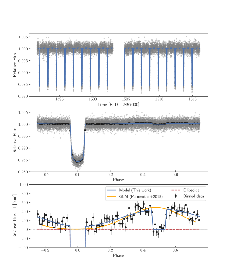
Figure 2: Top: the detrended TESS light curve of WASP-121 (grey) and the median model light curve drawn from the posterior (blue). Middle: The TESS phase curve of WASP-121 b. The grey points denote the raw light curve. Black points show the binned light curve. Blue line is the posterior median phase curve. Bottom: The TESS phase curve zoomed around unity showing the binned phase curve (black), the posterior median model (blue), ellipsoidal modulation (red dashed line), and, for comparison, a Global Circulation Model (GCM) prediction (Parmentier et al., 2018) (yellow line) (see Section 5). The grey centerline highlights zero, i.e., no emission from WASP-121 b.

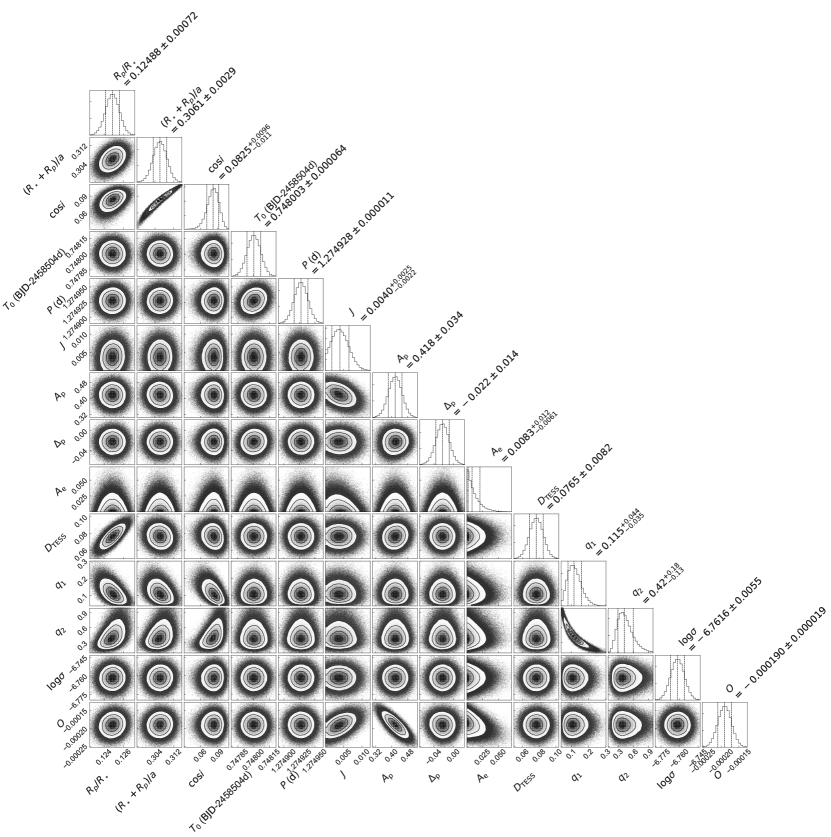
Figure 3: Posterior probability distribution of the light curve model parameters.

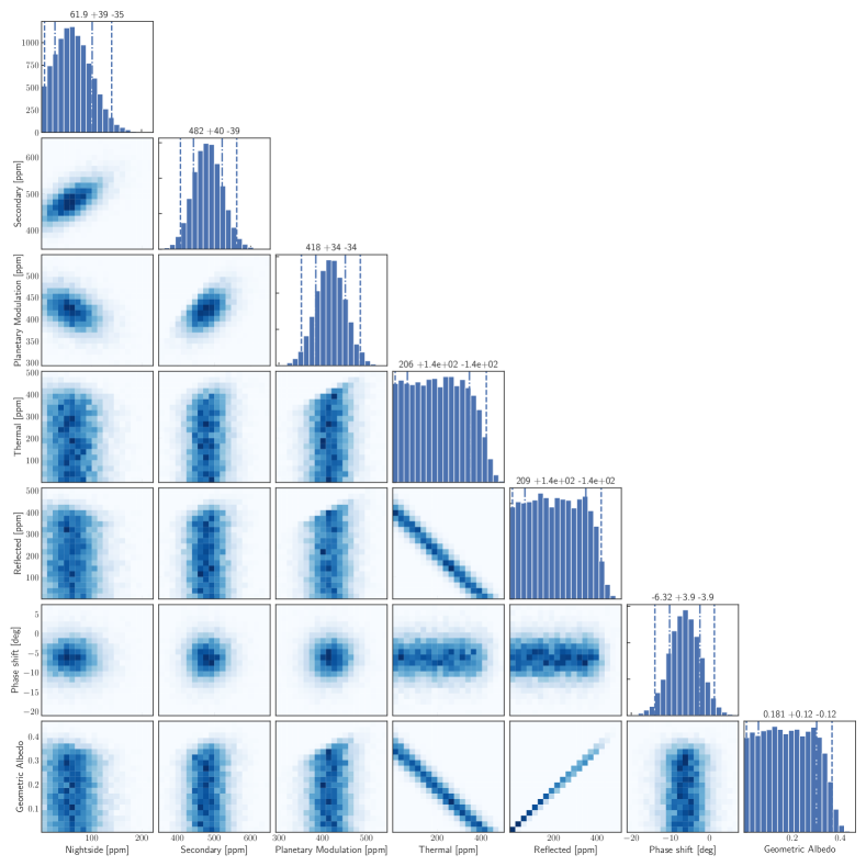
Figure 4: Joint posterior probability distribution of the derived parameters characterizing the WASP-121 b’s TESS phase curve. Dashed and dashed-dotted lines indicate 2$\sigma$ and $1\sigma$ credible intervals, respectively.

The measured red-optical secondary depth of WASP-121 b is in general agreement with the previous measurements (Delrez et al., 2016; Evans et al., 2017; Kovacs & Kovacs, 2019), as shown in Figure 7. However, based only on the retrieval analysis in Mikal-Evans et al. (2019), i.e., excluding this TESS measurement, we predict a secondary depth of $\sim$300 ppm. This implies that the TESS measurement of the secondary depth is above the expectation based on the measurements of the secondary in redder bands and that the dayside emission spectrum of WASP-121 b is inconsistent with that of a blackbody.

As for the nightside emission, we find a nightside brightness temperature of $2022\begin{subarray}{c}+254\\ -602\end{subarray}$ K for WASP-121 b and a westward phase shift of $6.3\begin{subarray}{c}+3.9\\ -3.9\end{subarray}$ degree, which is statistically consistent with zero. The measured nightside temperature implies a temperature contrast of $33\begin{subarray}{c}+20\\ -8\end{subarray}$%.

Using these inferences, we then solve for the two dimensional temperature distribution on WASP-121 b as shown in Figure 5, which illustrates the lack of the phase shift and reveals the large temperature gradient as a function of longitude. This picture is in contrast with the hot Jupiter HD 189733b, which has a thermal phase shift of $\sim 30$ degrees due to strong equatorial winds (Knutson et al., 2009).

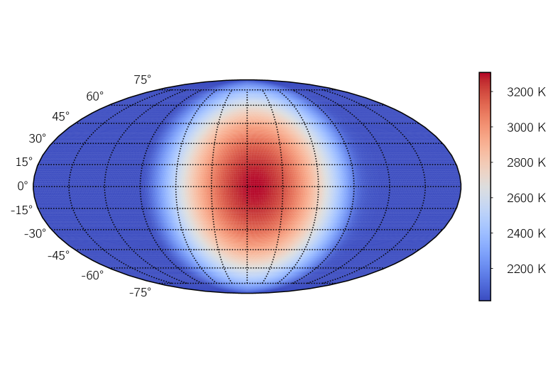
Figure 5: A two dimensional map of the temperature of WASP-121 b based on the best-fit solution to Equation 10.

4.2 Atmospheric characteristics

The posterior probability distribution of our ATMO parameters is given in Figure 6 and Table 3. With 44 degrees of freedom, we get a $\chi^{2}$ per degree of freedom of 1.05, indicating a good fit to the spectral data shown in Figure 7. We note that the discrepancy between the TESS depth and the bluest WFC3 G102 data is likely due to the fact TESS passband extends down to 0.6 $\mu$m and has contribution from species that WFC3 G102 is not sensitive to.

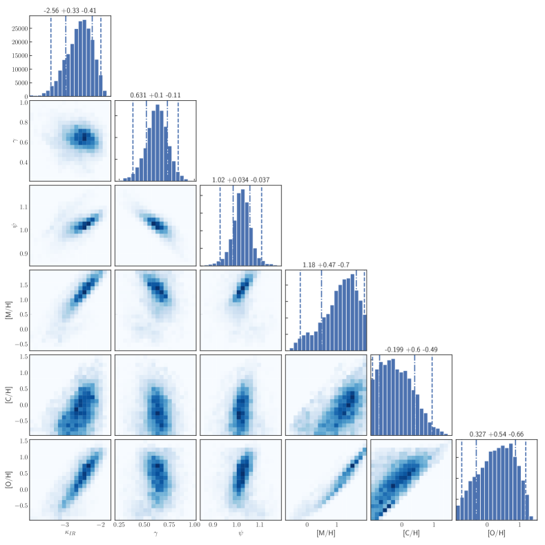
Figure 6: Joint posterior probability distribution of the ATMO parameters for the dayside atmosphere.

Name	Symbol	Value
Infrared opacity	$\kappa_{IR}$	$2.56\begin{subarray}{c}+0.33\\ -0.41\end{subarray}$
Optical to infrared opacity ratio	$\gamma$	$0.63\begin{subarray}{c}+0.10\\ -0.11\end{subarray}$
Irradiation efficiency	$\psi$	$1.02\begin{subarray}{c}+0.03\\ -0.04\end{subarray}$
Logarithm of the relative metallicity	[M/H]	$1.18\begin{subarray}{c}+0.47\\ -0.70\end{subarray}$ dex
Logarithm of the relative C abundance	[C/H]	$-0.20\begin{subarray}{c}+0.60\\ -0.49\end{subarray}$ dex
Logarithm of the relative O abundance	[O/H]	$1.33\begin{subarray}{c}+0.54\\ -0.66\end{subarray}$ dex

Table 3: Posterior median and 1$\sigma$ uncertainties of ATMO parameters.

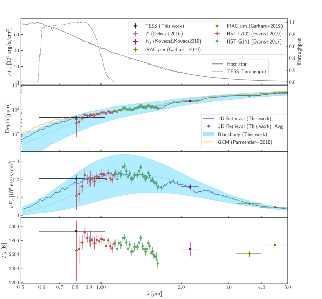
Figure 7: Top: The NextGen model spectrum of the host star, WASP-121 (continuous line) (Hauschildt et al., 1999) and the throughput of TESS (dashed line). Second from the top: The measured secondary depths of WASP-121 b including our atmospheric retrieval model (blue) and the blackbody model (light blue line and uncertainty band). For comparison, we also show the GCM prediction from Parmentier et al. (2018) (yellow). Second from the bottom: dayside emission spectrum of WASP-121 b. Bottom: inferred dayside brightness temperature.

The atmospheric retrieval indicates that the metallicity of the dayside atmosphere is $\sim$15 times that of the Sun, i.e., $1.18\begin{subarray}{c}+0.47\\ -0.7\end{subarray}$ dex. Furthermore, the abundance of carbon is not well-constrained, especially at the lower end, whereas that of oxygen is constrained to be near the Solar abundance. We note that our high metallicity constraint is not driven by the TESS data point. Indeed, as shown in (Mikal-Evans et al., 2019), atmospheric retrievals without the TESS data point also lead to high metallicities. The high metallicity is more likely driven by the red end of the HST data that have a steep downward slope reminiscent of the H^- bound-free opacity (Mikal-Evans et al., 2020).

The irradiation efficiency, $\psi$, of the dayside is also constrained near unity, indicating that the dayside atmosphere of WASP-121 b is consistent with being non-reflecting and has inefficient heat recirculation. In order to constrain the latter parameters, we use Equation 7 and Equation 9 to find the joint posterior probability distribution over the Bond albedo and the heat recirculation efficiency as shown in Figure 8.

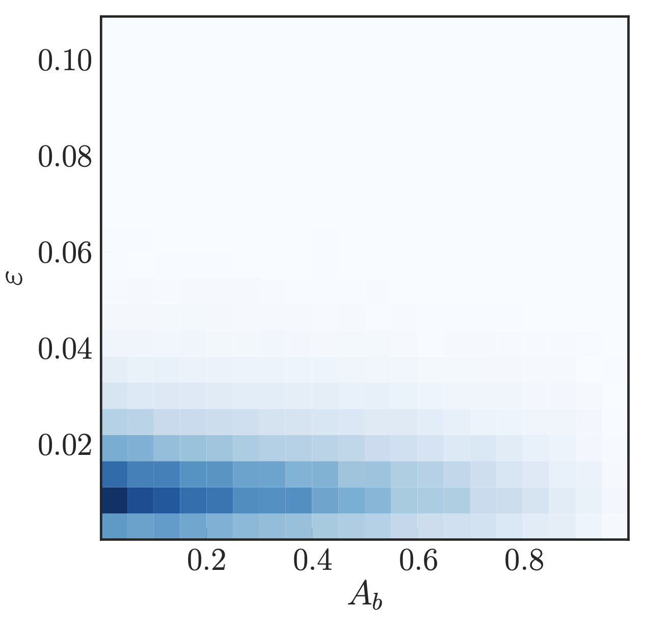
Figure 8: Joint posterior probability distribution of the Bond albedo, $A_{\rm B}$, and heat recirculation efficiency, $\varepsilon$.

Using the TESS-informed, predicted emission spectrum of WASP-121 b as shown in Figure 7, we then solve for the geometric albedo in the TESS passband. An estimate for WASP-121 b’s geometric albedo in the $z^{\prime}$ band was presented in (Mallonn et al., 2019) as $A_{\rm g}=0.16\pm 0.11$. We find a geometric albedo of $0.07\begin{subarray}{c}+0.037\\ -0.040\end{subarray}$ in the TESS band. This reveals mild (i.e., $\sim 2\sigma$) evidence that the atmosphere of WASP-121 b has non-negligible reflectivity in the TESS passband. Figure 9 compares the geometric albedo inferred based on only the TESS data and that inferred incorporating the thermal emission constraint from the atmospheric retrieval.

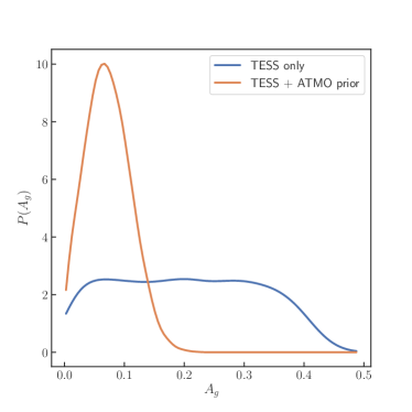
Figure 9: Posterior of the geometric albedo. The blue curve shows the albedo constraint obtained based only on the TESS phase curve. The yellow curve shows the posterior informed by the thermal emission prediction from ATMO.

The radiative transfer modeling also allows us to constrain the pressure-dependent temperature profile of the atmosphere, abundances of chemical species and the contribution function of TESS. In Figure 10, we present the pressure-temperature profile. In (Mikal-Evans et al., 2019) the atmospheric temperature was found to vary from 2500 K up to 2800 K from 30 mbar down to 5 mbar pressure. We find that the top of WASP-121 b’s atmosphere is hotter than previously thought and rises well above 3000 K.

The informativeness about the atmosphere of a given passband is encapsulated in a contribution function. This function indicates how much flux a particular wavelength interval contributes to each horizontal slice of the atmosphere.

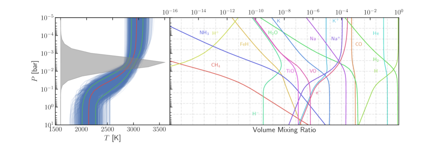
Figure 10: Left: Pressure-temperature profile of the dayside atmosphere of WASP-121 b. Blue lines are fair draws from the posterior, green lines are the 16th and 84th percentiles and the red line indicates the median. The superimposed filled grey curve shows the contribution function of TESS, revealing the altitude range for which the TESS data is informative. Right: Volume mixing ratios of various chemical species in the dayside atmosphere of WASP-121 b inferred based on the atmospheric retrieval.

We show in Figure 11 the abundance-weighted cross section of important species. We find that H^-, TiO and VO have the highest contribution to the opacity in the TESS passband at chemical equilibrium. The arrival of the TESS data raises their abundance-weighted cross section by roughly an order of magnitude and results in a dayside atmosphere with a much more pronounced temperature inversion.

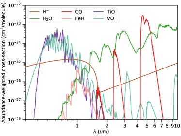
Figure 11: Cross sections of relevant species, weighted by their abundances at a pressure of 10 mbar. H^-, TiO and VO are the most important potential contributors to the opacity in the TESS passband.

5 Discussion

The TESS phase curve of WASP-121 b provides further evidence for the temperature inversion of its dayside atmosphere. The measured secondary depth also implies that the TESS secondary is deeper than expected based on previous measurements at longer wavelengths. There may be two components of this excess.

First, the planet may be reflecting some light in the TESS passband. Given that TESS passband covers shorter wavelengths, where the exoplanet-to-star contrast of thermal emission is lower, it is reasonable that this excess is due to reflected light from the exoplanet. In general, condensates such as H₂O and NH₃ on relatively cool (e.g., $\lesssim 300$ K) planets or condensates (e.g., silicates, Al₂O₃, CaTiO₃) on hotter planets (e.g., $\gtrsim 1500$ K) can make a planet reflective and result in a large albedo. However, ultra-hot Jupiters such as WASP-121 b are not expected to have a high reflectivity (Bell et al., 2017; Shporer et al., 2019) due to Mie scattering by clouds, because condensates required for this type of reflection would not form due to the high temperatures. Furthermore, cloud-free Rayleigh scattering is only effective at short wavelengths and would not be enough to increase the albedo to the inferred value in the TESS passband. However, despite the large substellar temperature of WASP-121 b, reflection can still happen from condensates on the western terminator (Parmentier et al., 2015).

Secondly, the excess may be due to additional sources of opacity in the dayside atmosphere of WASP-121 b with emission lines in the TESS passband, causing the planet to be heated at high altitudes. This would be consistent with earlier findings that there is a temperature inversion in the dayside atmosphere. This is also supported by our atmospheric retrieval, which predicts that the inversion in the pressure-temperature profile is more pronounced and that the atmosphere is hotter at high altitudes compared to Mikal-Evans et al. (2019). The potential temperature inversion is also consistent with the pressure temperature profile in Parmentier et al. (2018). Potential species that can cause this additional absorption are continuum opacity due to $H^{-}$, metals such as Fe gas (Lothringer et al., 2018), or band opacity due to TiO or VO. Although a minor effect, the internal heat of the planet might play a role in increasing the temperature as well. Finally, the presence of a spatially nonhomogeneous thermal structure on the dayside could be leading to an increase of the thermal emission at short wavelengths (Taylor et al., 2020).

The allowed range of heat recirculation can be explained as heat can be transported from the dayside to the nightside when molecular hydrogen, H₂, thermally dissociates into atomic hydrogen, H, recombines on the nightside into H₂, and releases internal energy. This process can make heat recirculation more efficient than that based on zonal jets only (Bell & Cowan, 2018; Komacek & Tan, 2018). A known trend in ultra-hot Jupiters is the increase of the day-night temperature contrast with the increase of dayside temperatures. This is due to the radiative time scale being too short in ultra-hot Jupiters (Komacek & Showman, 2016). The expected resulting dayside-to-nightside fractional temperature contrast for WASP-121 b is $\sim$30%, which is consistent with what we observe. We used Bell_EBM (Bell & Cowan, 2018) to model the energy balance of WASP-121 b including the effect of hydrogen dissociation and recombination. In this model, the predicted planetary modulation amplitude and phase shift are $\sim$600 ppm and $\sim$40 degrees eastward, respectively. The latter prediction is inconsistent with the observed phase shift and requires a non-negligible contribution from reflected light in the TESS passband, as also suggested by the fact that the secondary eclipse depth measured by TESS is larger than that predicted by ATMO based on multiband data. Our results indicate that WASP-121 b indeed has a phase shift consistent with zero. This could arise from competing phase shifts induced by the thermal and reflection processes mentioned above, which may be canceling each other.

We further compare our phase curve with the Global Circulation Models (GCMs) extensively described in Parmentier et al. (2018). The SPARC/MITgcm solves the primitive equation of hydrodynamics on a cube-sphere grid and the non-grey radiative transfer equations (Showman et al., 2009), assuming chemical equilibrium (including the thermal dissociation of molecules) and using the opacities from Freedman et al. (2014). The resulting outgoing flux is integrated over the TESS passband and compared to the observation in Figure 2. Despite its complexity the model presented here has several shortcomings: it neglects, among others, clouds, magneto-hydrodynamics effects and day/night latent heat transport through H₂ dissociation. Nonetheless, without adjusting any parameters the model predicts a reasonable phase curve amplitude in the TESS passband. In more detail, the model predicts a larger than observed phase curve offset and smaller than observed dayside flux. This could be the sign that magnetic drag is significantly slowing the winds of this planet compared to the simulation, as was proposed for WASP-18b (Arcangeli et al., 2019) and WASP-103b (Kreidberg et al., 2018). Additionally, the model underpredicts the nightside flux in the TESS passband, pointing towards the presence of an additional source of day-night heat transfer, most likely the transfer of energy through the latent heat of the dissociation/recombination of H₂.

The dayside emission spectrum predicted by the GCM also provides a good match to both the WFC3/G102 and the TESS data as shown in Figure 7. The red end of the WFC3/G121 dataset is poorly fitted by the GCM, which was already discussed in Parmentier et al. (2018) and Mikal-Evans et al. (2019). As shown by the retrievals, the WFC3/G121 datasets points toward a non-solar composition. An exploration of the parameter space with the GCM by varying the atmospheric metallicity and elemental abundance ratio would probably allow us to find a better match to the data, but is out of the scope of this paper.

The ellipsoidal variation was not measured to be statistically significant in the WASP-121 system. This amplitude of the ellipsoidal variation likely gets contributions from the tidal distortion of both the host star and WASP-121 b. The cross-sectional area for WASP-121 b should vary by $\sim$10% over the course of its orbit, implying that a large fraction of the ellipsoidal variation can be due to the tidal distortions of the planet (e.g., Kreidberg et al., 2018).

Future work on this system can potentially characterize the atmospheric temperature distribution to a greater detail (i.e., perform eclipse mapping) using GCMs. Magnetohydrodynamical (MHD) effects can also be investigated (Rogers & Showman, 2014), as WASP-121 b’s high substellar temperature causes a large amount of ionization as shown in the right panel of Figure 10.

6 Conclusion

In this work, we present the first analysis of the full phase curve of the ultra-hot Jupiter WASP-121 b as measured by TESS. We characterize the phase curve and the dayside atmospheric properties of WASP-121 b and find further evidence for its temperature inversion. We find that TESS observes excess emission from the dayside of WASP-121 b in the red-optical passband, which could be attributed to higher-than-expected reflected light or additional optically-thick absorbers in the red-optical band. We also measure the night-side emission, the temperature contrast, and the phase shift between the substellar point and the hot spot, finding that the heat transport on WASP-121 b must be inefficient.

References

- Agol et al. (2010) Agol, E., Cowan, N. B., Knutson, H. A., et al. 2010, The Astrophysical Journal, 721, 1861
- Amundsen et al. (2014) Amundsen, D. S., Baraffe, I., Tremblin, P., et al. 2014, A&A, 564, A59
- Angerhausen et al. (2015) Angerhausen, D., DeLarme, E., & Morse, J. A. 2015, Publications of the Astronomical Society of the Pacific, 127, 1113
- Arcangeli et al. (2018) Arcangeli, J., Désert, J.-M., Line, M. R., et al. 2018, ApJ, 855, L30
- Arcangeli et al. (2019) Arcangeli, J., Désert, J.-M., Parmentier, V., et al. 2019, A&A, 625, A136
- Bell & Cowan (2018) Bell, T. J., & Cowan, N. B. 2018, ApJ, 857, L20
- Bell et al. (2017) Bell, T. J., Nikolov, N., Cowan, N. B., et al. 2017, ApJ, 847, L2
- Charbonneau et al. (2005) Charbonneau, D., Allen, L. E., Megeath, S. T., et al. 2005, ApJ, 626, 523
- Claret (2017) Claret, A. 2017, A&A, 600, A30
- Cowan & Agol (2008) Cowan, N. B., & Agol, E. 2008, The Astrophysical Journal, 678, L129
- Cowan & Agol (2011) —. 2011, ApJ, 729, 54
- Delrez et al. (2016) Delrez, L., Santerne, A., Almenara, J.-M., et al. 2016, MNRAS, 458, 4025
- Drummond et al. (2016) Drummond, B., Tremblin, P., Baraffe, I., et al. 2016, A&A, 594, A69
- Evans et al. (2017) Evans, T. M., Sing, D. K., Kataria, T., et al. 2017, Nature, 548, 58
- Evans et al. (2018) Evans, T. M., Sing, D. K., Goyal, J. M., et al. 2018, AJ, 156, 283
- Foreman-Mackey (2016) Foreman-Mackey, D. 2016, The Journal of Open Source Software, 24, doi:10.21105/joss.00024
- Foreman-Mackey et al. (2017) Foreman-Mackey, D., Agol, E., Ambikasaran, S., & Angus, R. 2017, celerite: Scalable 1D Gaussian Processes in C++, Python, and Julia, Astrophysics Source Code Library, , , ascl:1709.008
- Foreman-Mackey et al. (2013) Foreman-Mackey, D., Hogg, D. W., Lang, D., & Goodman, J. 2013, PASP, 125, 306
- Freedman et al. (2014) Freedman, R. S., Lustig-Yaeger, J., Fortney, J. J., et al. 2014, ApJS, 214, 25
- Garhart et al. (2019) Garhart, E., Deming, D., Mandell, A., et al. 2019, arXiv e-prints, arXiv:1901.07040
- Goyal et al. (2017) Goyal, J. M., Mayne, N., Sing, D. K., et al. 2017, Monthly Notices of the Royal Astronomical Society, 474, 5158
- Guenther & Daylan (2020) Guenther, M. N., & Daylan, T. 2020, arXiv e-prints, arXiv:2003.14371
- Günther & Daylan (2019) Günther, M. N., & Daylan, T. 2019, allesfitter: Flexible star and exoplanet inference from photometry and radial velocity, Astrophysics Source Code Library, , , ascl:1903.003
- Hauschildt et al. (1999) Hauschildt, P. H., Allard, F., & Baron, E. 1999, ApJ, 512, 377
- Hunter (2007) Hunter, J. D. 2007, Computing in Science & Engineering, 9, 90
- Jenkins et al. (2010) Jenkins, J. M., Caldwell, D. A., Chandrasekaran, H., et al. 2010, ApJ, 713, L87
- Jenkins et al. (2016) Jenkins, J. M., Twicken, J. D., McCauliff, S., et al. 2016, in Proc. SPIE, Vol. 9913, Software and Cyberinfrastructure for Astronomy IV, 99133E
- Jones et al. (2001) Jones, E., Oliphant, T., Peterson, P., et al. 2001, SciPy: Open source scientific tools for Python, , , [Online; accessed 2017-02-07]
- Kipping (2013) Kipping, D. M. 2013, MNRAS, 435, 2152
- Knutson et al. (2009) Knutson, H. A., Charbonneau, D., Cowan, N. B., et al. 2009, ApJ, 690, 822
- Komacek & Showman (2016) Komacek, T. D., & Showman, A. P. 2016, ApJ, 821, 16
- Komacek & Tan (2018) Komacek, T. D., & Tan, X. 2018, Research Notes of the American Astronomical Society, 2, 36
- Kovacs & Kovacs (2019) Kovacs, G., & Kovacs, T. 2019, arXiv e-prints, arXiv:1901.02383
- Kreidberg et al. (2018) Kreidberg, L., Line, M. R., Parmentier, V., et al. 2018, AJ, 156, 17
- Line et al. (2013) Line, M. R., Wolf, A. S., Zhang, X., et al. 2013, ApJ, 775, 137
- Lothringer et al. (2018) Lothringer, J. D., Barman, T., & Koskinen, T. 2018, ApJ, 866, 27
- Mallonn et al. (2019) Mallonn, M., Köhler, J., Alexoudi, X., et al. 2019, A&A, 624, A62
- Mansfield et al. (2018) Mansfield, M., Bean, J. L., Line, M. R., et al. 2018, AJ, 156, 10
- Maxted (2016) Maxted, P. F. L. 2016, A&A, 591, A111
- Mazeh (2008) Mazeh, T. 2008, in EAS Publications Series, Vol. 29, EAS Publications Series, ed. M.-J. Goupil & J.-P. Zahn, 1–65
- Mikal-Evans et al. (2020) Mikal-Evans, T., Sing, D. K., Kataria, T., et al. 2020, MNRAS, 496, 1638
- Mikal-Evans et al. (2019) Mikal-Evans, T., Sing, D. K., Goyal, J., et al. 2019, MNRAS, 1700
- Morris (1985) Morris, S. L. 1985, ApJ, 295, 143
- Morris & Naftilan (1993) Morris, S. L., & Naftilan, S. A. 1993, ApJ, 419, 344
- Parmentier et al. (2016) Parmentier, V., Fortney, J. J., Showman, A. P., Morley, C., & Marley, M. S. 2016, ApJ, 828, 22
- Parmentier et al. (2015) Parmentier, V., Guillot, T., Fortney, J. J., & Marley, M. S. 2015, A&A, 574, A35
- Parmentier et al. (2018) Parmentier, V., Line, M. R., Bean, J. L., et al. 2018, A&A, 617, A110
- Ricker et al. (2014) Ricker, G. R., Winn, J. N., Vanderspek, R., et al. 2014, in SPIE Conf. Series, Vol. 9143, 20
- Rodler et al. (2010) Rodler, F., Kürster, M., & Henning, T. 2010, A&A, 514, A23
- Rogers & Showman (2014) Rogers, T. M., & Showman, A. P. 2014, ApJ, 782, L4
- Showman et al. (2009) Showman, A. P., Fortney, J. J., Lian, Y., et al. 2009, ApJ, 699, 564
- Shporer (2017) Shporer, A. 2017, PASP, 129, 072001
- Shporer et al. (2019) Shporer, A., Wong, I., Huang, C. X., et al. 2019, AJ, 157, 178
- Sing et al. (2019) Sing, D. K., Lavvas, P., Ballester, G. E., et al. 2019, The Astronomical Journal, 158, 91
- Smith et al. (2012) Smith, J. C., Stumpe, M. C., Van Cleve, J. E., et al. 2012, Publications of the Astronomical Society of the Pacific, 124, 1000
- Speagle (2019) Speagle, J. S. 2019, arXiv e-prints, 1904.02180
- Stassun et al. (2019) Stassun, K. G., Oelkers, R. J., Paegert, M., et al. 2019, AJ, 158, 138
- Stumpe et al. (2014) Stumpe, M. C., Smith, J. C., Catanzarite, J. H., et al. 2014, PASP, 126, 100
- Taylor et al. (2020) Taylor, J., Parmentier, V., Irwin, P. G. J., et al. 2020, MNRAS, 493, 4342
- Tremblin et al. (2016) Tremblin, P., Amundsen, D. S., Chabrier, G., et al. 2016, ApJ, 817, L19
- Tremblin et al. (2015) Tremblin, P., Amundsen, D. S., Mourier, P., et al. 2015, ApJ, 804, L17
- Tremblin et al. (2017) Tremblin, P., Chabrier, G., Mayne, N. J., et al. 2017, ApJ, 841, 30
- van der Walt et al. (2011) van der Walt, S., Colbert, S. C., & Varoquaux, G. 2011, Computing in Science & Engineering, 13, 22
- van Rossum (1995) van Rossum, G. 1995, Python tutorial, Tech. Rep. CS-R9526, Centrum voor Wiskunde en Informatica (CWI), Amsterdam
- Zhang et al. (2018) Zhang, M., Knutson, H. A., Kataria, T., et al. 2018, The Astronomical Journal, 155, 83
- Zhang & Showman (2017) Zhang, X., & Showman, A. P. 2017, ApJ, 836, 73