Evaluation of Automated Fermi GBM Localizations of Gamma-ray Bursts

Abstract

The capability of the Fermi Gamma-ray Burst Monitor (GBM) to localize gamma-ray bursts (GRBs) is evaluated for two different automated algorithms: the GBM Team’s RoboBA algorithm and the independently developed BALROG algorithm. Through a systematic study utilizing over 500 GRBs with known locations from instruments like Swift and the Fermi LAT, we directly compare the effectiveness of, and accurately estimate the systematic uncertainty for, both algorithms. We show simple adjustments to the GBM Team’s RoboBA, in operation since early 2016, yields significant improvement in the systematic uncertainty, removing the long tail identified in the systematic, and improves the overall accuracy. The systematic uncertainty for the updated RoboBA localizations is $1.8^{\circ}$ for 52% of GRBs and $4.1^{\circ}$ for the remaining 48%. Both from public reporting by BALROG and our systematic study, we find the systematic uncertainty of $1-2^{\circ}$ quoted in circulars for bright GRBs is an underestimate of the true magnitude of the systematic, which we find to be $2.7^{\circ}$ for 74% of GRBs and $33^{\circ}$ for the remaining 26%. We show that, once the systematic uncertainty is considered, the RoboBA 90% localization confidence regions can be more than an order of magnitude smaller in area than those produced by BALROG.

1 Introduction

To date, the Fermi Gamma-ray Burst Monitor (GBM; Meegan et al., 2009) is one of the most prolific instruments for the prompt detection of gamma-ray bursts (GRBs). Its onboard trigger algorithms detect $\sim 240$ GRBs per year, and for each of those, the Fermi GBM team sends public alerts within seconds of detection and transfers quicklook trigger data with a latency of $\sim 10$ minutes. This prompt public delivery of data has enabled community scientists rapid access to GBM data for triggered GRBs and has lead to several follow-up campaigns of GBM-detected GRBs as well as prompt correlation analysis between GBM triggers and triggers by other GRB-detecting instruments. Additionally, the full science data from GBM, both for onboard triggers and continuous data, is downlinked to the ground every few hours and is available publicly promptly after processing of the raw data into calibrated files. A top priority of the GBM Team is to provide such a rapid delivery of all data (typically $\ll 1$ day), enabling and encouraging community scientists to use GBM data for all manner of investigations, especially in the realm of time-critical observations and analysis.

In addition to the delivery of data for public use, one of the primary tasks of the Fermi GBM Team is to provide prompt localizations of GRBs detected by the GBM flight software. Unlike the Fermi Large Area Telescope (LAT) or the Neil Gehrels Swift Observatory, GBM does not have the capability of imaging or of reconstructing arrival directions of individual photons, and therefore it cannot consistently localize a signal on the sky to sub-degree precision. Instead, the localization method uses the relative rates of scintillation detectors oriented in different directions to estimate the source location, as pioneered by the KONUS experiments (Mazets et al., 1981). The GBM localization algorithm is based on that used for BATSE on the Compton Gamma-ray Observatory (Pendleton et al., 1999) and provides localizations for GBM with a statistical precision down to 1 degree and a typical localization region of several degrees in radius (Connaughton et al., 2015). What GBM lacks in precise localization power, however, it makes up with its all-sky monitoring capability, fine-time resolution, broad energy coverage, and fine spectral discrimination.

Localization of GRBs and other transients observed by GBM are of prime importance in the era of multi-messenger and time-domain astronomy. The benchmark example is the joint detection of GW170817 and GRB 170817A by LIGO/Virgo and Fermi GBM (Abbott et al., 2017a; Goldstein et al., 2017). These two detections of a binary neutron star merger in gravitational waves and gamma rays were entirely independent detections of the same event, and the consistent localization from both detections were an important piece in determining the high confidence of the connection between the two. Other examples include serendipitous observations of the sky or follow-up by other instruments. GRB 161228B was found by the intermediate Palomar Transient Factory (iPTF) to be a GRB counterpart to a Type IC broad-line Supernova, as discovered due to the localization agreement between the GRB and the supernova location (Corsi et al., 2017). iPTF and now its upgrade, the Zwicky Transient Facility, has followed-up GBM GRBs and discovered optical counterparts by utilizing only the GBM localizations (Singer et al., 2013, 2015; Coughlin et al., 2019). Other wide-field telescopes have begun follow-up as well, including MASTER (Lipunov et al., 2016), and GOTO (e.g. Mong et al., 2019; Ulaczyk et al., 2019). Finally, searches for counterparts to detections in other instruments, from radio to gamma-ray and including gravitational-wave and neutrino instruments, utilize GBM GRB localizations (Abbott et al., 2017b; Cunningham et al., 2019; Ho et al., 2019; Abbott et al., 2019).

To ensure that these and future efforts are productive, an accurate estimate of the GBM localization systematic uncertainty is a requirement to prevent reporting over-confident localizations that may result in false associations or lead to ruling out real associations. To that end, we determine with high fidelity the systematic uncertainty for two GBM localization algorithms: the GBM Team’s official automated system, termed the RoboBA, and the localization algorithm it uses, the DoL (Connaughton et al., 2015); and the independently developed BALROG algorithm (Burgess et al., 2017). Both of these algorithms use the real-time trigger data (TRIGDAT) provided by the onboard GBM flight software. The GBM flight software monitors the detector rates, and when it detects a statistically significant rate increase, it “triggers,” entering a mode that includes the production of special data. The trigger data includes onboard calculated localizations, which are constrained by using only a pre-burst background average and the severely limited onboard computational resources, and thus are less accurate but useful in the onboard classification of triggers. The TRIGDAT data also contains lightcurve data for quick look analysis. The TRIGDAT time history data extends from $\sim$130 s before the trigger to $\sim$470 s after the trigger, and is provided on timescales ranging from 64 ms to 8.192 s, with the shorter timescales concentrated around the trigger time. To transmit the TRIGDAT data in real time, the Fermi spacecraft initiates an unscheduled transmission with a NASA Tracking and Data Relay (TDRS) using the TDRS Demand Access Service. This service allows on-demand access, but provides only very low bandwidth. Collecting 470 s of data post-trigger, and transmitting the TRIGDAT takes 10 minutes – this dominates the latency of the RoboBA. The post-trigger data allows ground software to create background models using pre- and post-GRB data, which can result in significantly improved background estimates and thus improved localizations.

We first describe the RoboBA and BALROG algorithms in Sections 2 and 3, respectively, and then we discuss the methodology and samples of known GRB locations used to estimate the systematic uncertainty in Section 4. Finally, we discuss the overall results and implications in Section 5.

2 The Fermi GBM RoboBA

The RoboBA, operational since early 2016, is a set of algorithms developed to run autonomously to replace the Human-in-the-Loop (HitL) processing for most GBM GRB triggers. HitL processing requires burst advocates (BAs) to be on-call at all times and ready to promptly handle the processing of GBM triggers. Due to the increasing interest and importance in GBM-detected GRBs, localizations of GRBs are desirable as soon as possible. HitL processing had a median 1–2 hour delay in sending out final localizations, so the fully-automated RoboBA was developed to provide localizations for GRBs with accuracy on the order of human BA processing and a latency within 10 minutes after trigger (within seconds after complete receipt of TRIGDAT) and also reports in the GCN notice whether the GRB is likely to be a short or long duration GRB. The RoboBA has an automatic processing success rate of $\gtrsim 85\%$, with most failures due to dropped data packets in the real-time communication stream from the spacecraft. Since the first implementation in early 2016, there have been a few updates to the RoboBA, namely an update in early 2018 to provide localizations in full-sky HEALPix (Górski, et al., 2005) FITS files and an update in May 2019 to automatically send a GCN circular in addition to the machine-readable GCN notice (Fermi GBM, 2019a). We present here another update, implemented in September 2019, that further optimizes the performance of the RoboBA, resulting in overall improved localization accuracy and a smaller systematic uncertainty (Fermi GBM, 2019b). We first provide an overview of the RoboBA algorithm and then detail the most recent improvement in Section 2.5.

2.1 Background Estimation

The RoboBA, implemented in the GBM Burst Alert Pipeline (BAP), receives the real-time data as it arrives, sequences the data in the correct time order, and constructs the lightcurve. If the real-time trigger data is sufficiently complete, the RoboBA performs a series of background fits, utilizing a two-pass recursive non-parameteric regression. The non-parametric regression can accommodate a variety of non-stationary background conditions that are exhibited in GBM data, and it can handle the very limited amount of trigger data (usually $\sim 170$ time bins total). Since GRB lighcurves exhibit a wide variety of durations and morphologies, the regression is performed recursively, first fitting the full set of data, then removing bins from the background that exceed a predefined S/N threshold. The regression is repeated on the remaining time bins and those above the S/N threshold are removed until the recursive process converges, typically within 4 iterations. The first pass of this fit is performed on the sum of all energy channels for each detector to boost signal statistics. The second pass then performs the fitting process on each individual energy channel with the bins exceeding the S/N threshold already removed. Potential failures in the background fitting process are identified and reported to the human BA for inspection and manual localization. Failures in the background fitting typically only occur during extreme background variations and TRIGDAT truncation, which can occur when GBM triggers on a GRB as Fermi is entering or exiting the South Atlantic Anomaly.

2.2 Signal Identification

Once the background has been estimated, the signal needs to be identified. Because the primary goal is to perform a localization, and because the current GBM localization algorithm uses the signal in 50–300 keV energy range, we perform the following procedure utilizing only the data in that energy range. First, only considering the longer timescales in the TRIGDAT (8.192 s and 1.024 s), a calculation of each bin containing signal is performed assuming a mixture model of background+signal, with the signal model represented as an exponential function of signal counts during the trigger data window. This effectively assumes the background model is correct. Ideally, both background model and signal model would be simultaneously estimated, however the small number of time bins in TRIGDAT does not permit reliable convergence of such estimation for most GRBs. The prior assumption used in calculating the probability that a bin contains signal is approximately the fraction of bins above a predefined S/N threshold. The probability is calculated for each time bin in each detector and then the probabilities are combined across detectors such that incoherent background fluctuations in different detectors produce lower probabilities and coherent signal across detectors produce higher probabilities. Bins with a final probability $>0.89$ are considered as bins containing significant signal useful for localization. If the duration of the bins with significant signal is less than 2.1 s in duration, or if there is no identifiable signal on the longer timescales, then the shorter duration (64 ms and 256 ms) bins are considered and analyzed for the presence of a signal. If there is still no identifiable signal, then the RoboBA cannot proceed and the human BA is notified for a manual localization. This type of failure typically only occurs for extremely weak triggers or trigger with durations $<64$ ms (the GBM flight software can trigger on shorter timescales than are delivered in the TRIGDAT).

2.3 Signal Selection

Once the bins with likely signal presence have been identified, a selection can be determined for localization purposes. The GBM localization method is best performed when a contiguous segment of data has been identified and that segment is no longer than 30 s in duration. Signal selections longer than 30 s will typically result in a larger localization uncertainty due to the fact that the spacecraft is moving significantly relative to the GRB location, and the localization calculation is performed in the spacecraft frame. The RoboBA identifies the segment of the signal that contains the largest number of counts in order to minimize the statistical uncertainty of the localization, but will truncate the segment if it extends beyond 30 s in duration. The truncation is performed at either end of the segment, choosing to truncate the end that contains the fewest counts.

2.4 Localization and BAP Processing

Once the RoboBA has estimated the background and identified the signal for localization, the inputs are sent to the GBM localization algorithm called the DoL (Daughter of LOCBURST), which is an updated version of the localization code used by the BATSE Team to localize GRBs (Pendleton et al., 1999). The DoL assumes three spectral templates, selected to span the range of GRB spectra, and folds these template spectra through the NaI detector responses over a grid of points on the sky in the spacecraft frame. This produces model counts in each detector that is compared to the observed counts above background in each detector, which is done specifically in the 50–300 keV range for GRBs. Ultimately, the directional nature of the NaI responses and the blockage by the spacecraft body enable the localization of GRBs, since a specific region of the sky will produce a ratio of counts in the different detectors that match the observed ratio of counts. Connaughton et al. (2015) provides the full description of the algorithm and the initial estimate of the GBM localization systematic uncertainty related to this algorithm.

Once the DoL has provided the localization based on the inputs from the RoboBA, the BAP submits the GCN Notice and Circular for the RoboBA localization, and localization products, including the full-sky HEALPix map of the localization incorporating the estimated systematic uncertainty model, are uploaded to the HEASARC. The entire process of the RoboBA from receipt of the initial trigger packet to the sending of the GCN notice and circular takes 10 minutes, with virtually all of that time devoted to waiting for complete receipt of the data. Once the TRIGDAT packets have been received, the RoboBA completes its operations on the order of 1 second, and the DoL operates in $<10$ s on a single CPU. In addition to the public notices and maps, diagnostic lightcurves are produced for the human BA to verify the processing by the RoboBA, and examples are shown in Figure 1.

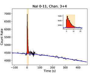
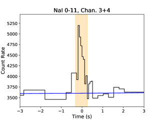
Figure 1: RoboBA processing of [Left] Fermi GBM long GRB 190222537 and [Right] short GRB 170817A. Shown is the sum of the data from all NaI detectors in the 50–300 keV energy range. The blue line is the background estimate, and the red filled region for the long GRB is identified as containing significant signal. The orange selection shows the segment of data chosen to perform the localization analysis.

2.5 Algorithm Improvements

The RoboBA algorithm was formulated and began operation prior to the production of the full-sky HEALPix maps, which provide a complete evaluation of the localization accuracy, precision, and systematics. Here we detail small improvements made to the RoboBA algorithm in order to make it more accurate and robust, and the evaluation of the systematic for these improvements are detailed in Section 4.3. One concern to be addressed by improving the RoboBA is the increased systematic uncertainty compared to the HitL, which the GBM Team accepted as a trade-off for the gain of prompt reporting (10 minutes instead of 1–2 hours). However, the most important property of the localization posterior is the total area once the systematic is incorporated, therefore only comparing the systematic uncertainty between the HitL and RoboBA localizations does not provide an accurate representation of the capability of the RoboBA. Therefore, we have undergone some review of the RoboBA algorithm, testing small changes to the parameters controlling its operation and testing changes to the three spectral templates used in the DoL, to provide an improvement in both accuracy and reliability.

The DoL, since beginning of GBM operations, has used three spectral templates for localization, all of the form of a Band function (Band et al., 1993). These are termed as ‘hard’, ‘normal,’ and ‘soft.’ Initially, testing focused on replacing the hard template, which has an unphysically hard high-energy power law, since it does not represent any known GRB spectrum. Testing on variations of the Band function yielded some improvement, however the most obvious improvement in localization accuracy resulted from replacing all Band function templates with cut-off power laws (commonly referred to as a Comptonized function, parameterized with $E_{\rm peak}$). The Comptonized parameters were then selected so that a majority of the GRB spectra would be represented by the normal spectrum, and the hard and soft spectra would represent the tails of the GRB spectral distribution. The parameters for the old Band function templates and the new Comptonized function templates are shown in Table 1.

Templates	Low-energy Index	High-energy Index	$E_{\rm peak}$ (keV)
Old Hard	0.0	-1.5	1000
Old Normal	-1.0	-2.3	230
Old Soft	-2.0	-3.4	70
New Hard	-0.25	-	1000
New Normal	-1.15	-	350
New Soft	-1.95	-	50

Table 1: The parameters of the old and new spectral templates used in the DoL for localization. The old templates were Band functions, and the new templates are Comptonized functions.

The RoboBA adjustments included improvements to the background fitting stability and robustness, allowing for a larger number of missing packets in the realtime TRIGDAT. The threshold to allow bins to be considered for localization was lowered from 89% to 75%, and the maximum duration of localization signal was shortened from 30 s to 15 s. Finally, the signal threshold for the short timescales was lowered from $3\sigma$ to $1.5\sigma$, reducing the failure rate for localizing weak short GRBs. All of these changes were relatively minor—an adjustment of a parameter in most cases—and included no additional complexity. The changes were tested on a sub-sample of GRBs with known locations (see Section 4.2) and validated on the remaining sample to ascertain an improvement in both localization accuracy and robustness. Indeed, after implementing these changes in the RoboBA and DoL, the localization accuracy and posterior sky area are now improved over even that of the HitL processing, with no added complexity or run-time. Additionally, the estimated failure rate is $<5\%$, reduced from $\sim 15\%$, largely due to ability to handle an increased number of dropped data packets. A few failures result from the misclassification of the GRB as ‘long’ or ‘short’ which determines the timescales of the TRIGDAT that are used for localization. By a simple comparison of the classification provided by the RoboBA to the final $\rm T_{90}=2$ s split, the RoboBA correctly classifies long GRBs 95% of the time and correctly classifies short GRBs 92% of the time. Not all misclassifications result in a localization failure, but they may require human follow-up to provide a more accurate localization. The remaining failures are dominated by severe TRIGDAT truncation and extreme background variability around entry and exit of the SAA. We detail the result of the improvements on the localizations in Section 4.3.

3 The BALROG algorithm

The BALROG algorithm (Burgess et al., 2017) is designed to provide a significant improvement for the GBM localization of GRBs by jointly fitting the GRB spectrum and position on the sky. In principle, fitting the spectrum allows a closer match to the true spectrum of the GRB and therefore should provide more accurate localizations with smaller systematic uncertainties. In practice, the BALROG algorithm performs a Monte Carlo sampling both on the sky and in spectral parameter space, using a parameterized spectral function. Per guidance from Berlato et al. (2019), three different spectral functions are tried (a power law, an exponentially cut-off power law, and a Band function), and the localization using the best-fit spectrum is selected. Unlike the RoboBA, which can run and produce a localization in $<10$ s on a single modern CPU, the BALROG algorithm requires the GBM detector responses to be generated for each Monte Carlo sample and therefore takes anywhere from an hour to a few hours to run using the three spectral functions on similar hardware. This implies the need for significant computing resources, such as a computing cluster, to produce localizations with a latency of several minutes.

For validation, the BALROG algorithm was tested specifically on bright GRBs with known locations, while weaker GRBs were not studied due to the assumption that systematic uncertainty is only a dominant contribution to the total uncertainty when the GRB is bright. Based on a subset of 69 localizations of bright GRBs originally presented in Connaughton et al. (2015), BALROG was shown to produce localizations with smaller angular offsets and significantly reduce the localization uncertainty, thereby making GBM localizations of GRBs both more accurate and more precise for most GRBs (Berlato et al., 2019). A slightly larger sample of GRBs (105) was used to estimate any remaining systematic uncertainty for BALROG. Berlato et al. (2019) determined that the remaining systematic was between $1-2^{\circ}$, with GRBs arriving along the direction of the Fermi solar panels tending to have the larger systematic than those arriving on the sides of the spacecraft where the GBM detectors were oriented. This remaining systematic was not rigorously or statistically estimated, but instead it was inferred visually and was intended only for an approximate comparison with the official GBM team localizations, not for use in assessing the true systematic. However, beginning on March 12, 2019, BALROG localizations relying on the GBM Team’s production of TRIGDAT began to be produced shortly after the trigger data became public (Greiner et al., 2019), utilizing the $1-2^{\circ}$ systematic.

3.1 Public Reporting

Since the beginning of public reporting of BALROG localizations through August 2019, there have been 23 GRBs with precise or well-constrained localizations from other instruments for which BALROG produced a public localization. While GCN circulars were not sent for all BALROG localizations, the localizations are available publicly on the MPE website and are accessible through the links provided in the GCN circulars (Greiner et al., 2019). The fact that the BALROG localizations are now produced with a small latency after the GBM Team localization allows for a near-realtime, blind, and unbiased comparison of how the localization algorithms fare. For the GBM Team localizations, GCN notices are sent for every localization and the localization files are hosted through the Fermi Science Support Center, and therefore the localizations have a public record. For the BALROG localizations, a record is available for those that have corresponding GCN circulars. In Table 2, we show the comparison between the RoboBA and BALROG localizations for these 23 GRBs. When GCN circulars are available for BALROG localizations, we use the information contained within, including the link to the HEALPix sky maps, while for the remaining GRBs we use the information publicly reported on their website. To establish a public record of the localization at, or near, the time that they were produced, we have archived the relevant BALROG webpages and to prevent confusion in case there are future updates to the localization. We note that care must be taken when retrieving the BALROG HEALPix sky map from the link in the GCN Notice, since it may retrieve the localization using TTE data instead of the TRIGDAT. In addition to the properties reported in Table 2, we include in the Appendix a sky map comparison of the RoboBA and BALROG localizations for this sample.

GRB	BALROG		GBM Team		Localizing Instrument
	Offset (deg)	Confidence Level	Offset (deg)	Confidence Level	(GCN)
190320A	2.47	0.04	7.90	0.79	Swift XRT (23977)
190324A	6.92∗	$1-(2\times 10^{-16})$	1.10	0.08	Swift UVOT (24014)
190331A	2.84	0.41	10.8	0.61	Swift BAT (24030)
190415A	4.25∗	0.994	2.81	0.44	IPN box† (24128)
190422A	18.95	1.00	3.34	0.43	Swift XRT (24151)
190427A	48.73	0.58	4.62	0.45	Swift BAT (24261)
190511A	7.12	0.84	4.71	0.76	Swift UVOT (24494)
190512A	36.63	0.98	3.71	0.24	Swift BAT (24520)
190515A	130.9	$1-(3.5\times 10^{-5})$	10.0	0.68	Fermi LAT (24560)
190519A	5.78	0.94	3.29	0.56	Swift XRT (24597)
190530A	0.64∗	0.45	3.34	0.46	Swift UVOT (24703)
190531B	2.94∗	0.66	4.05	0.52	Swift XRT (24706)
190606A	66.85	0.995	6.74	0.93	IPN box† (24765)
190613A	6.98∗	0.04	3.44	0.43	Swift UVOT (24815)
190613B	4.41∗	0.73	6.99	0.71	Swift UVOT (24817)
190719C	2.93	0.23	9.17	0.88	Swift XRT (25125)
190727B	1.97∗	0.83	4.65	0.76	Swift BAT (25211)
190731A	4.12	$1-(4\times 10^{-4})$	2.79	0.37	Swift XRT (25244)
190805B	4.33∗	$0.75$	2.44	0.26	IPN box† (25316)
190821A	12.1	0.98	5.60	0.31	Swift XRT (25436)
190824A	2.65	0.40	5.76	0.76	Swift XRT (25466)
190828B	12.6	0.21	5.41	0.80	Swift XRT (25521)
190829A	2.32	0.92	2.13	0.40	Swift XRT (25567)

Table 2: The list of GRBs with known or well-constrained locations for which the BALROG localization has been performed in near-real-time. The angular offset is calculated from the peak posterior density, and the confidence level is where the true location of the GRB is relative to the give localization posterior, including the prescribed systematic.
^∗ Reported in GCN: 190324A (23994), 190415A (24123), 190530A (24677), 190531B (24696), 190613A (24800), 190613B (24808), 190727B (25178), 190805B (25272)
^† Calculated from center of box

Table 2 lists the angular offsets of the peak probability density of each localization compared to the known location and the confidence level at which the true location lies, based on the posterior contained in the HEALPix files. Note that for both RoboBA and BALROG, the systematic uncertainty has already been incorporated, and in the case of BALROG, we use the systematic quoted in the GCN circular or the corresponding webpage. Of note is that the RoboBA localizations have a smaller offset from the true location for 15 out of the 23 GRBs, which is displayed in Figure 2, and that the BALROG excludes the true location at $\gtrsim 3\sigma$ for several GRBs, even though we include the prescribed systematic uncertainty. Figure 2 also shows the probability–probability plot comparing the calibrations of the RoboBA and BALROG localizations to expectations. For perfectly calibrated statistical and systematic uncertainties, the cumulative distribution of true locations within the GBM localization posterior confidence levels should approach that of a uniform distribution. That is, there should be a one-to-one relationship between the number of true locations that lie within a given confidence interval and the value of that confidence interval. For a finite sample size, especially a small sample size of 23, statistical fluctuations can cause significant deviation of the calibrated distribution away from the perfect assumption. Therefore, we sample from a uniform distribution of size 23 and empirically determine the 1, 2, and 3$\sigma$ (Gaussian equivalent) confidence intervals. We show the cumulative distributions for RoboBA and BALROG in comparison to these confidence intervals. While the localizations produced by the RoboBA keeps within $2\sigma$ of a well-calibrated uncertainty, the BALROG localizations deviate significantly beyond $3\sigma$, and in fact are inconsistent with a well-calibrated uncertainty at $>5\sigma$, indicating that the $1-2^{\circ}$ systematic claimed for BALROG is an underestimate of the true remaining systematic uncertainty. This underestimate is potentially problematic because any follow-up undertaken utilizing BALROG localizations has a good chance at searching an incorrect part of the sky.

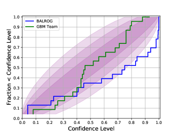
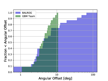
Figure 2: [Left] Cumulative distribution of the confidence level at which each of the known locations exist for the BALROG and RoboBA localizations. The purple bands represent the 1, 2, and 3$\sigma$ confidence regions for the expected equivalence of a perfectly calibrated localization uncertainty given a sample size of 23 GRBs. [Right] The cumulative distribution of angular offsets between the true location and the maximum density of the posteriors for RoboBA and BALROG.

3.2 Archival Testing

Due to the small sample size of known locations since BALROG began public reporting, we installed and ran the BALROG algorithm on a larger sample of archival GRBs with known locations. Following the BALROG tutorial and the steps and best practices outlined in Berlato et al. (2019), and with the desire to replicate the operational parameters of the real-time BALROG, we created a script to automatically process the necessary BALROG functions to localize a large number of GRBs with known locations. The entire process was performed blindly with respect to the true location for each GRB, as is done for the RoboBA. However, we note that initialization of the BALROG algorithm requires two additional pieces of information beyond what are available to RoboBA: a determination of the signal timescale and a selection for the set of detectors which are most likely to provide the best localization.

Unlike the RoboBA, which provides a classification on the type of GRB and therefore determines the timescale of data to use, the BALROG does not provide any automated identification of signal or signal timescale. This implies that either several selections must be attempted and evaluated based on some criteria, or that visual inspection is required to evaluate the appropriate duration of signal to choose. Due to computational considerations, we chose to identify the difference between long and short GRBs visually and select a signal interval of 8 s for long GRBs and a signal interval of 1–2 s for short GRBs. Once the signal selection had been performed, the background was then fit with a polynomial using a range of 100 seconds starting 20 seconds before the peak time bin and 50 seconds after, excluding the signal, to minimize source contamination in the background fit.

The guidance provided in Berlato et al. (2019) indicates that not all GBM detectors should be used by BALROG for localization in most cases, but instead only detectors within a certain angle from the true location should be used, or detectors from the side that is consistent with the arrival direction of the GRB should be used. Since, in a blind test, we cannot know a priori the true arrival direction of the GRB, we choose to use the 6 NaI detectors and BGO detector that are on the same side of the spacecraft as the detector with the highest count rate. We note that there are cases when the brightest detector does not necessarily indicate the general arrival direction of the GRB, such as in a case of high atmospheric scattering, but we choose this as our method so as to keep as close as possible to the operation of BALROG as outlined in Berlato et al. (2019).

Once the signal had been identified, the background fit, and the appropriate detectors selected, we initialized BALROG with a set of reasonable initialization parameters, and it performed the localization of the signal using three spectral forms: a Band function, Comptonized function, and a power law. As outlined in Burgess et al. (2017), the spectrum with the lowest $log(z)$ (the marginal log-likelihood) was chosen as the preferred spectrum, and the resulting RA and Dec chains from BALROG were formatted into a HEALPix FITS map. Several BALROG localizations failed to converge, at a rate consistent with what is produced by the automated BALROG pipeline (see Appendix 1 for some examples). In additional testing of the algorithm, we compared our results to those in Berlato et al. (2019), and while for many GRBs we could reproduce their results, there were several GRBs for which we could not reproduce their results unless manual selections of the signal were made until the localizations were consistent.

4 Localization Systematics Estimation

4.1 Methodology

The initial systematic uncertainty estimation for GBM localizations was described in detail in Connaughton et al. (2015). The method for evaluating the systematic uncertainty assumed that the localization statistical uncertainty was a von Mises-Fisher distribution (Gaussian distribution on a sphere). A Gaussian-equivalent 1$\sigma$ radius was calculated by determining the area of the $1\sigma$ region defined by the $\chi^{2}$ statistic produced from evaluating the localization fitness over a $1^{\circ}$ resolution grid on the sky. Various models for the systematic uncertainty were compared with a Bayesian technique, optimizing the parameters of each model using the log-likelihood and comparing models by odds ratios. The probability of each localization was determined, and included in the likelihood, by using the distance of the GBM localization from a point source localization from another instrument or distance from an IPN (Hurley et al., 2013) localization annulus. This technique was originally developed to estimate the systematic uncertainty of BATSE GRB localizations (Briggs et al., 1999). This method found that there was evidence for a two-component systematic, termed a ‘core+tail’ model, which is a sum of two von Mises-Fisher distributions. There was also evidence that the systematic was different for two distinct slices in spacecraft azimuth, indicating directions in the spacecraft frame where there is a smaller systematic uncertainty. In general Connaughton et al. (2015) found that the ‘core’ contribution to the model ($\sim$88–92% contribution) has a systematic defined by a 1$\sigma$ radius of 2.3–4.2 degrees and the ‘tail’ contribution has a radius of 13.2–15.3 degrees. Note that since the core+tail model is an empirical estimation of the systematic that is not motivated by known contributors, one cannot predict a priori which GRB localization will be represented by the ‘core’ component of the systematic or the ‘tail.’ Therefore, the systematic uncertainty is a mixture of the two components and is convolved with the statistical uncertainty to produce the final calibrated uncertainty.

The assumed circular approximation for the localization uncertainty, however, is not accurate in many cases. In practice, the statistical uncertainty of the localization can be quite complex, affected by the blockage of the detector fields by parts of the spacecraft, scattering of photons from the spacecraft, and backscattering of photons from the atmosphere. Imperfect knowledge of the spacecraft mass model, the atmospheric scattering model, and the true spectrum of the source (as well as its inherent spectral evolution) all contribute to the systematic uncertainty, and each of these contributions are difficult to isolate, deconvolve, and correct. We can evaluate the overall effectiveness of the systematic model, and thereby the Gaussian assumption, by performing a convolution of the systematic model with the statistical uncertainty and producing a probability-probability (P–P) plot, as was shown in Figure 2.

The P–P plot is a widely-used tool to investigate the similarity of two cumulative distributions. In the context of measuring the contribution of systematic uncertainty to the estimation of a set of random variables, the P–P plot is useful in comparing the ensemble of proposed posteriors to the expected fraction of true values within specified confidence levels in the frequentist interpretation. For example, if we calculate the localization posterior for a sample of GRBs of which we know the true location, the P–P plot allows us to determine if 50% of the true locations fall inside the 50% confidence region, 90% of the true locations fall inside the 90% confidence region, etc. A unity line is often shown to establish the expected comparison, and a deficit in comparison to that line indicates that the posterior, on average, underestimates the uncertainty, while an excess over that line indicates an overestimate of the uncertainty. In short, the P–P plot indicates the integrity of an uncertainty calibration.

Since the P–P plot is a measure of the calibration of the posterior, continuous along all confidence values, it can be used to estimate a systematic component of the posterior when a statistical estimate of the posterior underestimates the true uncertainty. This is useful whether or not the sources of systematic uncertainty are known, and whether or not several sources can be easily disentangled and modeled. Generally, if one has a model for the systematic which has some free parameters, to calibrate the systematic against the P–P plot, the binomial likelihood function must be maximized:

$$L(p|n,y)\propto p^{y}(1-p)^{(n-y)},$$ (1)

where $p$ is the binomial probability, $n$ is the number of trials in a given experiment, and $y$ is the number of “successes” in that experiment. The binomial log-likelihood of $n$ events with a given “success rate” and expected probability along the P-P plot is:

$$\ln{L}\propto\sum_{i=0}^{n}y_{i}\ln{p_{i}}+(n-y_{i})\ln(1-p_{i}),$$ (2)

and in this context we define success rate as the number of true locations within a given confidence level. In terms of the P–P plot, at any point along the cumulative distribution, one is measuring the number of “successes” given the data and comparing it to the expected number of successes from the model of the uncertainty. To estimate the parameters of a systematic uncertainty model, we maximize the binomial log-likelihood, which cannot be solved analytically in this situation. Since the statistical uncertainty for a GBM localization can have a wide variety of morphologies without a standard analytical description, we must choose an optimization algorithm that will determine the parameter values that maximize the likelihood.

We choose to use the Nelder-Mead simplex algorithm (Nelder & Mead, 1965) to minimize the negative log-likelihood by convolving a candidate systematic model with the statistical posterior for each GRB in the sample. The fitting process proceeds as:

1. Initialize the systematic model with a guess parameter vector;

2. Convolve each GRB localization posterior with the systematic model;

3. Construct the cumulative distribution of the fraction of true locations within the confidence regions;

4. Calculate the negative binomial log-likelihood and evaluate the Nelder-Mead stopping criteria;

5. If the Nelder-Mead stopping criteria hasn’t been satisfied, the Nelder-Mead algorithm formulates a new parameter vector and steps 2–4 are repeated until convergence.

Once the fitting process has concluded, the minimum of the negative log-likelihood has been found. By assuming that likelihood surface in the region local to the minimum is approximately Gaussian, the covariance matrix of the fit can be estimated by calculating the inverse of the Fisher Information Matrix, $I(\theta)$, for the log-likelihood, which is the negative Hessian of the log-likelihood as a function of the systematic model parameters, $\theta$:

$$\Sigma=[I(\theta)_{i,j}]^{-1}=E\biggl{[}-\frac{\partial^{2}}{\partial\theta_{i}\partial\theta_{j}}\ln{L(X;\theta)}\biggr{|}\theta\biggr{]}^{-1}.$$ (3)

In the case of the GBM localization posteriors, since the likelihood depends on the statistical uncertainty, which has no analytical form, we use finite differences to estimate the elements of the Hessian.

4.2 Sample

To evaluate the efficacy of the current and updated RoboBA localization systematic and the BALROG systematic, we use a sample of 516 GRBs with locations known to a 1-$\sigma$ precision of $\leq 1^{\circ}$ as determined by other instruments. This sample represents a selection of GRBs spanning from the beginning of GBM operations in July 2008 through March 2019, and was gathered from the online GBM GRB catalog. This represents a factor $>2.5$ larger sample compared to the constrained locations used in Connaughton et al. (2015) and a factor $\sim 5$ larger sample compared to Berlato et al. (2019), and combined with our improvements in methodology, we can create an increasingly robust estimation of the localization systematic uncertainty for both algorithms.

For both the RoboBA and the BALROG  we ran this sample of GRBs through automated processing blindly, without considering the known location. In the case of the RoboBA, the algorithm as implemented in the BAP was run on a desktop computer over all GRBs in the sample, meanwhile, we utilized the Alabama Supercomputer to run the BALROG algorithm so that the localizations could be performed in a tractable amount of time. In both cases there were a few failures of the algorithms to identify and localize signals. The RoboBA identified 11 failures out of the sample of 516, therefore we exclude those failures from consideration. For BALROG, 17 failures were immediately identified that prevented the algorithm from completing, therefore we exclude those GRBs from the BALROG sample. Additionally, several BALROG localizations would not converge, and no identifiable cause was found other than sensitivity to initial conditions. We exclude these 103 GRBs from consideration for BALROG, leaving a sample of 396 GRBs. We use the full sample of successful localizations to estimate the systematic for each algorithm, and we use the sub-sample of joint successes for the head-to-head comparisons.

4.3 RoboBA Results

The RoboBA localizations were fit using the prescribed methods, first starting with a single Gaussian representing the systematic for all GRBs, and then with the ‘core+tail’ model. In all cases, the single Gaussian systematic is not sufficient to accurately describe the systematic, therefore the preferred model for the systematic is the ‘core+tail’ model. For the original RoboBA algorithm, the systematic was calibrated with a smaller sample of GRBs under the Gaussian assumption used in Connaughton et al. (2015). In initial testing of the RoboBA, it was determined that the systematic was noticeably larger for short GRBs than for long GRBs, and since the majority of GRBs detected by GBM are long, the systematic underestimated the true uncertainty for localizations of short GRBs. Therefore, we estimated the systematic for long and short GRBs (as classified by RoboBA) separately, and show those models in Table 3 in comparison to the HitL systematic. While the RoboBA localizations do not exhibit a $>10^{\circ}$ tail for long GRBs as was estimated for the HitL localization, the short GRBs localizations are contaminated with a small fraction of very bad localizations, producing a tail that extends out to $\sim 30^{\circ}$. Improvements to the RoboBA were specifically targeted at solving this tail, along with generally reducing the overall systematic.

Model	Sample	Core (∘)	Core %	Tail (∘)
HitL	All GRBs	$3.7\pm 0.2$	$90\pm 4$	$14\pm 3$
	Az: $292.5-67.5^{\circ}$ & $112.5-247.5^{\circ}$	$4.2\pm 0.3$	$92\pm 4$	$15\pm 4$
	Az: $67.5-112.5^{\circ}$ & $247.5-292.5^{\circ}$	$2.3\pm 0.4$	$88\pm 6$	$13\pm 4$
Original RoboBA	Long GRBs	$2.6\pm 0.1$	$65\pm 4$	$6.0\pm 1.0$
	Short GRBs	$3.6\pm 0.1$	$98\pm 1$	$29.6\pm 15.6$
Updated RoboBA	All GRBs	$1.81\pm 0.02$	$51.7\pm 1.2$	$4.07\pm 0.05$
	Long GRBs	$1.86\pm 0.02$	$57.9\pm 1.2$	$4.14\pm 0.06$
	Short GRBs	$2.55\pm 0.08$	$39.0\pm 1.2$	$4.43\pm 0.16$
	Hard Spectrum	$2.38\pm 0.07$	$52.8\pm 0.9$	$4.97\pm 0.12$
	Normal Spectrum	$1.94\pm 0.04$	$62.4\pm 0.6$	$3.44\pm 0.09$
	Soft Spectrum	$1.40\pm 0.03$	$40.4\pm 0.6$	$4.05\pm 0.06$

Table 3: The systematic uncertainty models for the HitL, original, and updated RoboBA.

Considering the updated RoboBA, we are afforded the opportunity to test different hypotheses on the sources of the systematic with such a large sample of GRBs. As was shown in Connaughton et al. (2015) and later in Berlato et al. (2019), there is evidence for an azimuthal dependence of the systematic in spacecraft coordinates, which would imply an angular-dependent systematic in the GBM detector responses. Since identifying and correcting a putative systematic in the response is outside the scope of this work, and since the arrival direction of a GRB is not known a priori in useful circumstances, modeling the systematic as a function of arrival direction provides a poor predictive solution. Instead, we aim to further model the systematic based on the characteristics of the RoboBA so that those characteristics can be used to leverage a more accurate and optimal estimate of the systematic on a per-GRB basis. Specifically, we investigate the systematic resulting from the different preferred spectral templates, since a source of systematic can be the imperfect assumption of the spectrum for the GRB (Burgess et al., 2017; Berlato et al., 2019). We also investigate the systematic for what the RoboBA algorithm determines are long and short GRBs, as was done for the original RoboBA. Since the RoboBA makes a classification of the GRB, and the signal identification and selection methodology is somewhat different between what the RoboBA determines is a long or short GRB, there can be different contributions of systematic uncertainty due to the methodology.

For estimating the systematic between RoboBA-identified long and short GRBs, we divide the sample and fit each separately: 431 long GRBs and 74 short GRBs. The resulting best-fit systematic models are shown in Table 3. Similar to the overall systematic uncertainty estimation, the ratio of GRBs in the core and tail are $\sim$1:1, and the long GRBs overall have a smaller systematic uncertainty compared the short GRBs. The reason for this could be due to the difference in methodology, or it could be due to the fact that long and short GRBs have different spectra and short GRBs will tend to have a larger systematic if the hard spectrum results in a larger systematic. Addressing the latter hypothesis, we divide the complete sample based on which spectral template was identified as most appropriate for localization. This results in 145 GRBs with the hard template, 236 GRBs with the normal template, and 124 with the soft template. We fit each of these separately and find good fits with the ‘core+tail’ model for each. Indeed, the hard template has the largest associated systematic, likely due to the fact that the atmospheric scattering component has a larger contribution to the response for harder spectra, thereby making the localization more sensitive to the assumed spectral shape. All three systematic calibrations are approximately equivalent and are shown in Figure 3. As a matter of convenience, we choose to use the long/short systematic model for the new RoboBA throughout the rest of this work as well as in our implementation of the updates, since our RoboBA data pipeline is already configured to handle a short/long systematic model. We may consider refining this decision in the future to further improve the estimate of the systematic on an individual GRB basis.

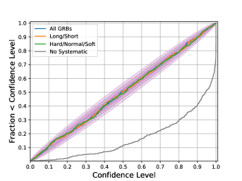
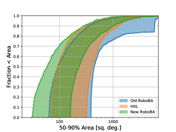
Figure 3: [Left] The calibration of the RoboBA systematic as evaluated over 505 GRBs, splitting into long and short GRB samples, and splitting into hard, normal, and soft spectra. The distribution with no systematic is shown for comparison. The purple contours denote the empirical 1, 2, and 3$\sigma$ confidence levels for the calibration. [Right] Cumulative distributions of the 50% (dashed line) credible area and 90% (solid line) credible area for the old and new RoboBA and the HitL localizations.

While the systematic uncertainty we estimate here is smaller for the new version of the RoboBA compared to the original RoboBA and the HitL localization, a more important metric of localization improvement is the total area of the localization posterior once the systematic component is included. We show in Figure 3 the comparison of the 50% and 90% credible region areas on the sky between the original and updated RoboBA and the HitL. Note that the HitL localizations are not precisely of the same GRBs, since HitL localizations are rarely performed since 2016, but they were chosen randomly from the pre-2016 set of GRBs. Immediately obvious is the reduction in area on the sky with the new version of the RoboBA. The median improvement in the 50% credible region area is from $\sim 80\ \rm deg^{2}$ to $\sim 50\ \rm deg^{2}$, while the median improvement in the 90% credible region area is from $\sim 400\ \rm deg^{2}$ to $\sim 200\ \rm deg^{2}$. This improvement in the new RoboBA is not only due to resolving the long tail in the systematic, but is a result of an overall improvement in the accuracy of the RoboBA and DoL to localize GRBs.

4.4 BALROG Results

For BALROG, we can first use this method to estimate the systematic on the public automated localizations performed by BALROG since March 2019. Performing the maximum likelihood estimation, we find that the systematic is likely represented by a mixture of Gaussians, similar to the ‘core+tail’ model discussed earlier. The core Gaussian has $\sim 2.4^{\circ}$ radius, representing $\sim 82\%$ of the localizations and the remaining 18% of localizations exhibit a $\sim 32^{\circ}$ tail. The fit results, including testing a single Gaussian fit is shown in Table 4, while the calibration including this systematic model is shown in Figure 4.

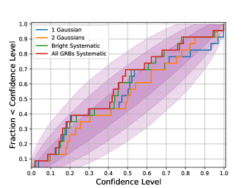
Figure 4: The probability plot for the publicly reported BALROG localizations using an estimated systematic models incorporating a single Gaussian and a mixture of two Gaussians. The two Gaussian ‘core+tail‘ model appears to be favored. The systematic models estimated for the bright sample and complete sample of GRBs are consistent with that observed for the publicly reported sample within 2$\sigma$.

Sample (# GRBs)	Model	Core (∘)	Core %	Tail (∘)	Log-Like
Realtime (23)	Single Gaussian	$3.5\pm 0.1$	–	–	–285
	Core+Tail	$2.4\pm 0.1$	$82\pm 4$	$32\pm 6$	–267
All GRBs (396)	Single Gaussian	$6.58\pm 0.01$	–	–	–87516
	Core+Tail	$3.08\pm 0.03$	$74.9\pm 0.3$	$33.3\pm 0.6$	–78911
Bright GRBs (230)	Single Gaussian	$5.60\pm 0.02$	–	–	–32051
	Core+Tail	$2.68\pm 0.03$	$73.6\pm 0.5$	$32.9\pm 1.2$	–26716
Weak GRBs (166)	Single Gaussian	$8.22\pm 0.09$	–	–	–14246
	Core+Tail	$5.44\pm 0.29$	$83.7\pm 1.7$	$37.5\pm 0.9$	–13800

Table 4: The estimated systematic uncertainty for BALROG with different samples

Similarly, this analysis can be performed on a larger sample of GRBs to provide a better constraint on the systematic and to check consistency with the real-time sample. Since Berlato et al. (2019) defined a ‘bright’ GRB threshold and compiled a sub-sample of GRBs that satisfied that threshold to perform the comparison against the GBM Team’s localizations, we use the same definition for the bright sample:

$$F_{\rm peak}>(6\ {\rm ph\ cm^{-2}\ s^{-1}})-(0.857\times 10^{5}\ {\rm erg^{-1}\ s^{-1}})\ S,$$ (4)

where $F_{\rm peak}$ is the 1-s peak photon flux and $S$ is the energy fluence in 10-1000 keV. This results in 230 GRBs from the sample described in Section 4.2. It is important to note that this brightness cut over-samples long GRBs relative to short GRBs as there are only 14 short GRBs in this sample that satisfy the bright criteria. As a first check of accuracy, we show the head-to-head comparison of the angular offsets of the peak posterior density from the true location between RoboBA and BALROG in Figure 5. For all but a few percent of the bright GRBs, RoboBA has a small angular offset, with a median offset of $\sim 3^{\circ}$ and a maximum of $\sim 20^{\circ}$. BALROG, however, has a median offset of $\sim 6^{\circ}$ and a long tail of very large offsets out to $\sim 120^{\circ}$. Note that this long tail is not a consequence of failed convergence, as those have been removed from the sample; the tail appears to be due to localizations that converged to a completely incorrect part of the sky.

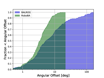
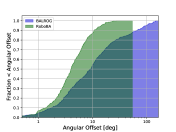
Figure 5: Comparison of the angular offsets from the known location between RoboBA and BALROG for the [Left] bright sample and [Right] complete sample of GRBs. The long tail in the BALROG distribution is from localizations that converged to a completely incorrect part of the sky.

While the angular offset distribution is consistent with that observed by the real-time localizations shown in Figure 2, we can also check consistency of the systematic uncertainty for this larger sample. We fit the ‘core+tail’ model to these GRBs and find that 74% of the bright GRBs have a $2.7^{\circ}$ systematic and the remaining 26% have a $33^{\circ}$ systematic. This systematic model is broadly consistent with that found for the real-time localizations, as shown in Figure 4. It is not immediately obvious what causes the long tail in the systematic for BALROG, since Burgess et al. (2017) and Berlato et al. (2019) stated that simultaneously fitting the spectrum and location should solve the long tail for previous GBM localizations, however there is strong evidence that this tail is present both in our study as well as the localizations produced in near real-time and distributed publicly. By applying this more constrained systematic model to the localization posteriors, when can compute the localization area, which is one of the most important figures of merit for GBM localizations. We show in Figure 6 the comparison of the RoboBA and BALROG 50% and 90% credible region areas for both the real-time GRBs and the bright sample.

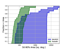
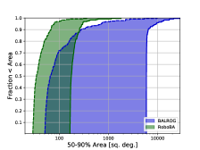
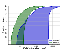
Figure 6: Cumulative distributions of the area for the 50%–90% confidence region for the public automated localizations [Left] for the RoboBA and BALROG, the bright sample [Middle], and the full sample [Right] by applying the corresponding systematics.

We also estimate the systematic for the full sample of GRBs described in Section 4.2. While bright GRBs are considered to be the most affected by systematics, we find that the systematic uncertainty is slightly larger when considering the full sample. This is likely due to the fact that background modeling and signal selection are increasingly important for weak GRBs and are of lesser consequence for very bright GRBs, thereby causing different sources of systematic to arise based on the observed brightness of the GRB. This systematic is still broadly consistent with the real-time localizations, but it is a slightly less favorable match than the bright systematic. The cause of the increased systematic appears to be due to the converse of the bright sample, the ‘weak’ sample of GRBs as the fit parameters show in Table 4. Indeed, BALROG appears to perform systematically worse for weaker GRBs, possibly a consequence of imprecisely modeling the background, and not carefully minimizing background contamination in the signal selection. Nominally, for statistically-limited signals, the statistical uncertainty should be larger than bright signals, however, it appears that BALROG is relatively more overconfident for weaker signals than for bright signals.

5 Discussion

Through a quantitative estimation of the systematic uncertainty for the RoboBA and BALROG localizations, we compared the robustness and accuracy of the two algorithms. Compiled in Table 5 are a number of summary values for the two methods. The RoboBA is found to be more accurate at localizing GRBs, and is even more accurate with the newest updates detailed in Section 2.5. Theoretically, it is reasonable to expect that simultaneously estimating the source spectrum and localization would solve some of the systematic uncertainty in GBM localizations, and we find that the different spectral templates the DoL uses do indeed produce different systematics. Clearly if the assumed spectrum is enormously different from the true spectrum, inaccuracies in the localization can be produced, however it is not clear how close the proposed spectrum needs to be to the true spectrum to eliminate this systematic. Burgess et al. (2017) discusses the fact that the simultaneous fitting of the spectrum and location can lead to an increase in the area of the statistical uncertainty because it is a more accurate representation of the true uncertainty. There is evidence that this increase in the statistical uncertainty occurs for most BALROG localizations, however, there is still a considerable systematic uncertainty that exists, a larger systematic than even for the localizations produced by the RoboBA. In Figure 7 we show an example of what the localization posteriors look like for an average GRB in the bright sample, once the appropriate systematics are considered.

	Original RoboBA	Updated RoboBA	BALROG
Systematic Model	long (short)	long (short)	all (bright)
Core (deg.)	2.6 (3.6)	1.86 (2.55)	3.1 (2.7)
Core Fraction (%)	65 (98)	57.9 (39.0)	74.9 (73.6)
Tail (deg.)	6.0 (29.6)	4.14 (4.43)	33.3 (32.9)
Angular Offset	all (bright)	all (bright)	all (bright)
Median	$4.3^{\circ}$ ($3.7^{\circ}$)	$4.1^{\circ}$ ($3.5^{\circ}$)	$9.7^{\circ}$ ($5.4^{\circ}$)
90% Range	$1.3-15^{\circ}$ ($1.1-11^{\circ}$)	$1.0-15^{\circ}$ ($0.9-10^{\circ}$)	$1.2-99^{\circ}$ ($1.0-90^{\circ}$)
50% Area (sq. deg.)	all (bright)	all (bright)	all (bright)
Median	83 (69)	49 (34)	151 (66)
90% Range	64–461 (64–140)	29–330 (29-78)	65–2228 (51–717)
90% Area (sq. deg.)	all (bright)	all (bright)	all (bright)
Median	423 (395)	209 (175)	5834 (5936)
90% Range	386–5982 (386–5867)	166–1138 (165–299)	5756–13507 (5925–9494)
Failure Rate	$\lesssim 15\%$	$\lesssim 5\%$	$\sim 15-20\%$
CPU Time	$\lesssim 10$ s	$\lesssim 10$ s	O(hours)

Table 5: Summary statistics of the old RoboBA, updated RoboBA, and BALROG localizations. The 90% range represents the range of values spanning 5%–95% of the cumulative distribution.

It is beyond the scope of this work to pinpoint the sources of this additional systematic within BALROG, but it is worth noting the convergence and sensitivity issues that can arise with the BALROG algorithm. For a number of GRBs, the convergence of the localization to the true location is sensitive to the initial conditions, either the initial parameters of Monte Carlo chains or the background fit and signal selection. Indeed, by studying the results from the online version of BALROG, similar issues with convergence appears as well, particularly for weaker and/or short GRBs. While this can be diagnosed and amended for GRBs with known locations, BALROG is only of use for localization if one doesn’t know the location a priori. Our failure rate of $\sim 23\%$ in running BALROG may be higher than that of the online version ($\sim 15-20\%$) even though we followed the guidance and tutorials and attempted to replicate the process of the online algorithm. Potential sources of the differences may lie in our methodology in selecting the detectors to use for each GRB. If that is the case, then the online version of BALROG may be utilizing additional information, such as the location provided by the GBM Team as was suggested in Berlato et al. (2019). Nevertheless, the fact that our study of BALROG localizations finds a systematic consistent with what is being produced by the online version suggests that these failures do not significantly affect our determination of the overall accuracy of BALROG. Both the automated localizations produced by BALROG and our larger study disagree quite strongly with the $1-2^{\circ}$ systematic quote for BALROG. This appears to indicate a difference in methodology between the study performed by Berlato et al. (2019) and what is currently implemented for BALROG. It may be possible to produce a much better localization with BALROG if the background, signal selection, and detectors can be tuned for a given GRB, however, that requires considerable input by a human.

Considering that valuable telescope time will be used to follow up GBM GRB localizations, it is important that the community have the best information on the accuracy of the available algorithms. Our results show that the GBM Team’s current localizations, primarily those from RoboBA, are more accurate on average than BALROG, require a smaller systematic uncertainty, have a considerably smaller area covered by the localization posterior, are more robust against failure, and are more computationally efficient leading to a smaller reporting latency. Furthermore, given that the systematic uncertainty provided publicly for BALROG considerably underestimates the uncertainty achieved, there is risk of follow-up observations tiling incorrect regions of the sky. Similarly, spatially correlative studies are at risk of finding false correlations, or missing real correlations, due to the underestimated systematic. Implementation of improvements to RoboBA have significantly improved its accuracy and have reduced the sky area for follow-up searches, and we will continue to investigate additional improvements to the RoboBA and DoL algorithms.

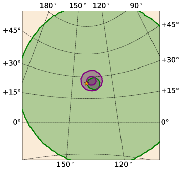
Figure 7: An example comparison of localization posteriors for RoboBA (purple) and BALROG (green) once the appropriate systematic models are considered. The 50% and 90% regions are shown, and the true location, determined by the Fermi LAT, is marked with the gold star. This localization, of GRB 170522A, is slightly worse than the median angular offset for RoboBA, and is slightly better than the median angular offset for BALROG.

6 Appendix

The following figures are sky maps comparing the localizations from the original RoboBA and BALROG algorithms for each of the 23 GRBs contained in Table 2. The BALROG localizations shown here are from the BALROG webpage reporting their near-realtime results, and we incorporate the prescribed systematic as determined on the corresponding webpage or GCN notice. The 50% and 90% confidence regions are shown for both algorithms, the GBM RoboBA localizations are represented by the purple filled contours, and the BALROG localizations are represented by green contours. The known location of each GRB is marked by a black star. As can be seen, 9–10 of the known locations exist outside the BALROG 90% confidence region, while only one of the known locations exists outside the RoboBA 90% confidence region (GRB 190606A). Additionally, it appears there are 2 non-convergent localizations produced by BALROG: GRBs 190515A and 190606A, and another poorly-converged localization: GRB 190828B.

References

- Abbott et al. (2017a) Abbott, B, P., et al. 2017, ApJ, 848, L13
- Abbott et al. (2017b) Abbott, B, P., et al. 2017, ApJ, 841, 89
- Abbott et al. (2019) Abbott, B, P., et al. 2019, arXiv:1907.01443
- Band et al. (1993) Band, D., Matteson J., Ford, L., et al. 1993, ApJ, 413, 281
- Berlato et al. (2019) Berlato, F., Greiner, J., & Burgess, J. M. 2019, ApJ, 873, 16
- Briggs et al. (1999) Briggs M. S., Pendleton G. N., Kippen R. M., Brainerd J. J., Hurley K., Connaughton V., Meegan C. A., ApJS, 122, 503
- Burgess et al. (2017) Burgess, J. M., Yu, H.-F., Greiner J., & Mortlock, D. J. 2017, MNRAS, 476, 1427
- Connaughton et al. (2015) Connaughton, V. C., Briggs, M. S., Goldstein, A., et al. 2015, ApJS, 216, 32
- Corsi et al. (2017) Corsi A., Cenko, S. B., Kasliwal, M. M., et al. 2017, ApJ, 847, 54
- Coughlin et al. (2019) Coughlin, M. W., Ahumada, T., Cenko, S. B., et al. 2019, PASP, 131, 048001
- Cunningham et al. (2019) Cunningham, V., Cenko, S. B., Burns E. et al. 2019, ApJ, 879, 40
- Fermi GBM (2019a) Fermi GBM 2019, GCN Circ 24408
- Fermi GBM (2019b) Fermi GBM 2019, GCN Circ 25726
- Goldstein et al. (2017) Goldstein, A., Veres, P., Burns, E., et al. 2017, ApJ, 848, L14
- Górski, et al. (2005) Górski, K. M., Hivon, E., Banday A. J., et al. 2005, ApJ, 622, 759
- Greiner et al. (2019) Greiner J., Biltzinger, B., Kunzweiler, F., Berlato F., & Burgess, J. M. 2019, GCN Circ 23956
- Ho et al. (2019) Ho A. Y. Q., Goldstein D. A., Schulze, S. et al. 2019, arXiv:1904.11009
- Hurley et al. (2013) Hurley, K., Pal’shin, V. D., Aptekar, R. L., et al. 2013, ApJS, 207, 39
- Lipunov et al. (2016) Lipunov V. M., Gorosabel J., Pruzhinskaya M. V., et al. 2016, MNRAS, 455, 712
- Mazets et al. (1981) Mazets E. P., Golenetskii S. V., 1981, Astrophysics and Space Science, 75, 47
- Meegan et al. (2009) Meegan, C., Lichti, G., Bhat, P. N., et al. 2009, ApJ, 702, 791
- Mong et al. (2019) Mong Y. L., Ackley, K., Kennedy, M. et al. 2019, GCN Circ 24425
- Nelder & Mead (1965) Nelder, J. A. & Mead, R. 1965, Computer Journal, 7, 308
- Pendleton et al. (1999) Pendleton, G. N., Briggs, M. S., Kippen, R. M., Paciesas, W. S., Stollberg, M. & Woods, P. 1999, ApJ, 512, 362
- Singer et al. (2013) Singer, L. P., Cenko, S. B., Kasliwal, M. M., et al. 2013, ApJ, 776, L34
- Singer et al. (2015) Singer, L. P., Kasliwal, M. M., Cenko, S. B., 2015, ApJ, 806, 52
- Ulaczyk et al. (2019) Ulaczyk K., Lyman, J., Steeghs, D. et al. 2019, GCN Circ 24432
- Vianello et al. (2015) Vianello. G., Lauer, R. J., Younk, P. et al. 2015, arXiv:1507.08343