Reality as a simulation of reality: robot illusions,
fundamental limits, and a physical demonstration

Abstract

We consider problems in which robots conspire to present a view of the world that differs from reality. The inquiry is motivated by the problem of validating robot behavior physically despite there being a discrepancy between the robots we have at hand and those we wish to study, or the environment for testing that is available versus that which is desired, or other potential mismatches in this vein. After formulating the concept of a convincing illusion, essentially a notion of system simulation that takes place in the real world, we examine the implications of this type of simulability in terms of infrastructure requirements. Time is one important resource: some robots may be able to simulate some others but, perhaps, only at a rate that is slower than real-time. This difference gives a way of relating the simulating and the simulated systems in a form that is relative. We establish some theorems, including one with the flavor of an impossibility result, and providing several examples throughout. Finally, we present data from a simple multi-robot experiment based on this theory, with a robot navigating amid an unbounded field of obstacles.

“Truth is beautiful, without doubt; but so are lies.”— Ralph Waldo Emerson

I Motivation and Overview

Robotics papers usually include evidence of algorithms or controllers that have been executed or evaluated on some kind of system, typically comprising either physical robots or a substitute. But what constitutes a robot demonstration, exactly? One division is generally drawn between software simulation and real robots. This is, at best, a rather rough distinction for there is a spectrum of simulators spanning a wide range of fidelities. Actually, the same might be said for physical robots: data and conclusions from robots using, say, a sophisticated external motion capture system, or cameras with visual markers, might be representative of robots operating in the field with GPS. Or, on the other hand, depending on what you’re trying to do, they might not.

What is certain is that there are more choices, between full software simulation and full physical implementation, than are generally recognized or garner attention (see Figure 1). Inasmuch as this is critical for robotics as a scientific enterprise, it is perhaps curious that there has been little formal treatment of representativeness or verisimilitude beyond the complete hardware and software extremes, and their consideration. This paper’s raison d’être is to initiate a close, systematic examination of these other options.

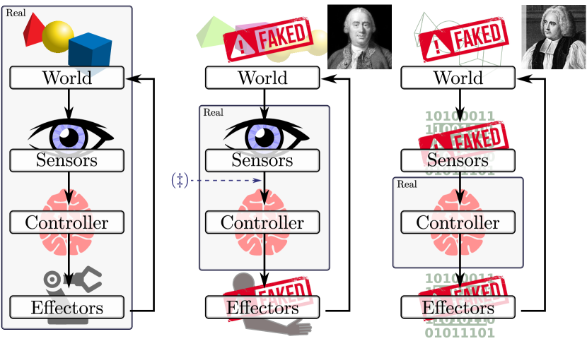
Figure 1: An illustration of different modes of fakery matched with appropriate intellectual positions: the orthodox view (left) and two forms of philosophical skepticism (center and right). The left column represents an end-to-end physical robot experiment with every part being real. The middle column, bearing the bust of David Hume, involves real sensors but also reason to doubt the veracity of the world they report. The rightmost column, headed by Bishop Berkeley, has a real controller but all other elements are mere software—it represents a robot experiment conducted in simulation (for the commonplace use of that term) where information is injected directly into the robot’s cortex. Hume’s column is the case studied in the paper: robots perceive a world mediated by sensors that are grounded in the real world, but it is a world of “nothing but sophistry and illusion.”

We want to understand how one physical system may be used to mimic the behavior of another. By system, we are considering a setting where observations are made (via sensors) and used to choose actions that are effected (via actuators) and this unfolds over time. We begin with a simplified discrete-time setting (Definition 1) where we can contemplate exact emulation (Definition 2), rather than considering approximate or imprecise imitation. The central features which distinguish the approach from other formalisms of emulation between robot systems (see Section II) are the possibility of variable time expansion (somewhat akin to Milner’s weak bisimulation [21]) and a narrow focus on mimickry only up to the perceptual capabilities of the system under emulation.

We then formulate some particular questions, such as: “What are the resources involved, how do we quantify resource requirements, and relate them?” (Definition 3, Theorem 4), “How do we compose or nest such systems?” (Theorem 2), “What happens to these things when systems are modified (Theorem 3)”, etc. Even this simple setting is replete with possibilities, some of which are both exciting and enticing (Section VII).

In terms of immediate utility for the practitioner, the present paper shows how to conduct a novel sort of emulation with real hardware where sensors, rather than being faked out of whole cloth—as is usually done with computational or mathematical models that are highly idealized coarse approximations—provide real signals. As the instances we study herein show, there may be considerable freedom in choosing different ways to emulate one system with another, with implications for future robotic laboratory infrastructure.

II Related work

II-A Animal studies: The inspiration for the present work

For decades, biologists have sought to chart the perceptual limits of organisms and to understand how informational mismatches affect behavior [39, 9]. Recent years have seen virtual and augmented reality technologies being used in this quest with considerable enthusiasm. The animals studied range from small mammals [12] down to insects [36], being studied both while walking [35] and flying [10, 11, 18]. The journal Current Zoology recently devoted a special issue to the topic [40]. As a concrete example, Takalo et al. constructed a laboratory apparatus comprising a spherical projection surface and a track ball that enables the detailed study of the walking behavior of the cockroach (periplaneta americana) by providing it with synthetic visual stimuli, ultimately to give a systems-level understanding of the organism [35].

II-B Practical simulation in software

Software simulations are an inescapable part of the current robotics research landscape, with the community devoting much time and attention to related questions, including through the biennial simpar conference. The software traces out some element of a robot’s execution in a virtual, rather than physical world, generating artificial sensor readings (or sometimes state information), and evolving the robot system forward in time.

Center to most discussions about software simulation are considerations of fidelity: How closely does the simulator mimic the real world? High-fidelity simulation software like Gazebo [14] has been developed to account for many of the complications experienced by the complex robots native to many research labs. But fidelity may be traded for other features as some efforts strike a “useful balance between fidelity and abstraction” [38]. Other simulators, designed for specific robot types [13, 6, 30, 27, 7, 32], optimization/control schemes [37], and application domains [2, 23, 31], exist.

This work is partly a generalization of the traditional notion of robot simulation, but with elements of the simulation conducted physically rather than virtually. Closely related work includes endeavors that alter aspects of the physical world using mixed or augmented reality techniques [1, 33, 4, 3]. The distinguishing here is that modifications of the world are made by robots and for robots, not human developers or operators, and not via additional display technologies.

II-C Simulation as theoretical concept

Relating systems by the fact that they can simulate each other, for some definition of simulation, is a recurring theoretical theme. The symmetric notion, where two systems are each able to match the other, yields the concept of bisimulation, which is an equivalence relation. Bisimilarity was identified independently in modeling concurrent systems [20] and in modal logic [26]; it also has a game theoretic interpretation [34].

Closer to home in robotics, invariants among sensori-computation circuits of Donald [8], and the dominance relation between robot systems introduced by O’Kane and LaValle [25], bear parallels to the notion of illusion we introduce here, particularly in the use of one system, or re-arrangements of the resources contained therein, to emulate certain properties of another. In this paper, the emphasis on perceptual equivalence for the robots participating in the illusion is fresh.

III Preliminary definitions

III-A Systems

We wish to talk about relationships between pairs of systems of robots. First, then, we need to define the notion of a system. Because henceforward we shall consider systems consisting of possibly many robots, we jump directly into definitions that consider (potentially) multiple robots. Superscripts in parentheses denote robot indices; subscripts are time indices.

Definition 1.

A deterministic multi-robot transition system is a $7$-tuple $(n,X,U,f,Y,h,x_{0})$, in which

1. $n$ is a positive integer identifying the number of robots,

2. $X=X^{(1)}\times\cdots\times X^{(n)}$ denotes a state space, composed of individual state spaces for each robot,

3. $U=U^{(1)}\times\cdots\times U^{(n)}$ denotes an action space, composed of individual action spaces for each robot,

4. $f:X\times U\to X$ is a state transition function, defined in terms of transition functions $f^{(1)},\ldots,f^{(n)}$ for each robot, so that

   $$f \left((x^{(1)},\ldots,x^{(n)}),(u^{(1)},\ldots,u^{(n)})\right)$$

   $$=\left(f^{(1)}(x,u^{(1)}),\ldots,f^{(n)}(x,u^{(n)})\right).$$

5. $Y=Y^{(1)}\times\cdots\times Y^{(n)}$ denotes an observation space, composed of individual observation spaces,

6. $h:X\to Y$ is an observation function, defined in terms of observation functions $h^{(1)},\ldots,h^{(n)}$ for each robot, so that $h\left(x\right)=\left(h^{(1)}(x),\ldots,h^{(n)}(x)\right)$,

7. $x_{0}\in X$ is the system’s initial state.

Such a system evolves, in a series of discrete time steps, subject to the following pair of equations:

$$X\hskip 11.0pt \hskip 22.0ptX\hskip 9.0ptU$$

$$x_{k+1} =f(x_{k},u_{k}),$$

$$y_{k} =h(x_{k}).$$

$$Y\hskip 1.0pt \hskip 22.0ptX$$

Figure 2: An example of the sort of system in Example 1, with $n=4$. At each time step $k$, each robot is at some point $x^{(i)}_{k}$ along the roadway moving with velocity $u^{(i)}_{k}$, and measures the distances $y^{(i)}_{k}$ to the adjacent robots.

A few simple examples, to be revisited later, illustrate the idea.

Example 1.

Consider a caravan of $n$ autonomous vehicles —that is, robots— moving down a long single-lane roadway. Suppose each robot can control its own velocity, subject to some upper and lower bounds, and can also measure the distance to the other robots immediately in front of and immediately behind itself. See Figure 2. We might describe this scenario as a deterministic multi-robot transition system

$$S_{n,v_{\rm min},v_{\rm max}}=(n,\mathbb{R}^{n},[v_{\rm min},v_{\rm max}]^{n},f,\mathbb{R}^{+}\times\mathbb{R}^{+},h,x_{0}),\vspace*{-2pt}$$ (1)

for which we’ll give the state transition function $f$ and observation $h$ shortly. Here elements of the state space $X=\mathbb{R}^{n}$ encode the position, along the one-dimensional roadway, of each of the $n$ robots. At each time step $k$, the action $u^{(i)}_{k}\in[v_{\rm min},v_{\rm max}]$ of robot $i$ denotes the velocity of that robot at that time. Thus, we may define $f(x,u)=x+u$. We assume that $v_{\rm min}<v_{\rm max}$. Each observation $y^{(i)}_{k}\in\mathbb{R}^{+}\times\mathbb{R}^{+}$ is a pair of integers indicating the distance to the closest other robot, if any, in each direction:

$$y^{(i)}_{k}\!=\!h^{(i)}(x_{k})\!=\!\bigg{(}\!\! \min\left(\!\left\{|x^{(j)}_{k}-x^{(i)}_{k}|\middle|x^{(j)}_{k}<x^{(i)}_{k}\right\}\cup\{\infty\}\right),$$

$$\min\left(\!\left\{|x^{(j)}_{k}-x^{(i)}_{k}|\middle|x^{(j)}_{k}>x^{(i)}_{k}\right\}\cup\{\infty\}\right)\!\!\bigg{)}.\vspace*{-2pt}$$

To refer to the individual measurements in a single observation, we use the symbols $b$ and $a$ for the distances behind and ahead, so that $y^{(i)}_{k}=(b^{(i)}_{k},a^{(i)}_{k})$. Finally, the initial state $x_{0}$ is some known but arbitrary state.

Notice that (1) is, in fact, defining an infinite family of systems, parameterized by the number of vehicles in the system and the ranges of allowable velocities.

This is, of course, a heavily idealized model of caravaning autonomous vehicles, crafted as an elementary illustration of Definition 1. Richer models might, for example, expand $X$ to model multi-lane roadways or the robots’ lateral positions within the lanes, enrich $U$ and $f$ to model the dynamics of some physical system more faithfully, or modify $Y$ and $h$ to model, say, a lidar sensor with greater fidelity.

Example 2.

Consider a system in which many small disk-shaped differential drive robots move in a shared, bounded, planar workspace, with each robot aware of the relative positions of the other robots within some small sensor range. Refer to Figure 3[left]. One might realize this kind of system using, for example, Khepera [22], r-one [19], or GRITSbot [28] robots. We can model such a system by choosing the number of robots $n$, the rectangular workspace $W\subseteq\mathbb{R}^{2}$, the maximum wheel velocity $v_{\rm max}$, and the sensor range $r$. We then define

$$S_{\text{disks}}=\left(n,X_{\text{disks}},U_{\text{disks}},f_{\text{disks}},Y_{\text{disks}},h_{\text{disks}},x_{0}\right),\vspace*{-4pt}$$ (2)

in which the states in $X_{\rm disks}=(W\times S^{1})^{n}$, the actions in $U_{\rm disks}=[-v_{\rm max},v_{\rm max}]^{2}$ denote the left and right wheel velocities for each robots, the state transition function $f_{\text{disks}}$ encodes the well-known kinematics for differential drive robots, the observations in $Y_{\text{disks}}=\cup_{i=0}^{n-1}(\mathbb{R}^{2})^{n}$ are lists of between $0$ and $n-1$ planar positions, the observation function $h^{(i)}_{\text{disks}}$ for each robot $i$ returns a list of the relative positions of any other robots within distance $r$ of robot $i$, and the initial state $x_{0}\in X_{\text{disks}}$ is a known but arbitrary state.

Example 3.

Definition 1 is also suitable for describing single-robot systems as a particular case with $n=1$. For example, a velocity-controlled robot moving in a very large field of nearly-identical static obstacles, with a sensor to detect those obstacles when they are nearby, might be modelled as

$$S_{\text{single}}=\left(1,X_{\text{single}},U_{\text{single}},f_{\text{single}},Y_{\text{single}},h_{\text{single}},x_{0}\right),\vspace*{-2pt}$$ (3)

with $X_{\text{single}}=\mathbb{R}^{2}$, $U_{\text{single}}=[-v_{\rm max},v_{\rm max}]$, and $f_{\text{single}}(x,u)=x+u$. The observation space $Y_{\text{single}}$ and $h_{\text{single}}$ may be defined to return the locations of the center points of each obstacle. See Figure 3[right].

\begin{picture}(1919.0,1197.0)(3038.0,-3298.0)\end{picture}

\begin{picture}(1881.0,1054.0)(3078.0,-3408.0)\end{picture}

Figure 3: [left] A team of simple robots in a bounded environment, as in Example 2. [right] A single robot moving in a unbounded field of obstacles, as in Example 3.

III-B Policies

In the model, a robot operates by choosing actions to execute, a concept detailed via a policy. The essential question in formalizing policies is to determine what information is used by the robot in considering its action. Now, to define the policy concept, we adopt the style of LaValle’s book [16].

We begin, first, with something simple that will turn out to be inadequate for our needs. If robot $i$, at time step $k$, has sufficient information that it can determine its state, i.e., it is a fully observable problem, then its policy $\pi^{(i)}$ might be defined as a function of that state:

$$X^{(i)} \hskip 26.0ptU^{(i)}$$

$$x^{(i)}_{k} \xmapsto{\pi^{(i)}}u^{(i)}_{k}.\vspace*{-4pt}$$ (4)

More likely, the robot will only have access to its history of actions and observations to select its action

$$U^{(i)}\hskip 18.0ptU^{(i)}\hskip 6.0ptY^{(i)}\hskip 16.0ptY^{(i)} \hskip 26.0ptU^{(i)}$$

$$u^{(i)}_{0},\dots,u^{(i)}_{k},y^{(i)}_{0},\dots,y^{(i)}_{k} \xmapsto{\pi^{(i)}}u^{(i)}_{k}.$$ (5)

In what follows, one robot system will seek to present some view of the world to match a description as will be seen by some other, secondary system. This primary system must know some aspects of that other system to fool it effectively. That is, the primary system must be aware of the ‘fourth wall’ and know some of the expectations and qualities on the other side of it. Throughout, we use a notational convention: we distinguish the primary system (initially best thought of as the physical system) by placing a hat over its variables; all variables for the secondary are bare. Now, returning to our formalization of the policy concept, we must generalize the notation so far in order for it to present information about the primary system and a secondary one, partitioned like such

$$\widehat{U}^{(i)}\hskip 18.0pt\widehat{U}^{(i)}\hskip 6.0pt\widehat{Y}^{(i)}\hskip 18.0pt\widehat{Y}^{(i)}\hskip 3.0ptX\hskip 22.0ptX\hskip 2.0pt \hskip 24.0pt\widehat{U}^{(i)}$$

$$\widehat{u}^{(i)}_{0},\dots,\widehat{u}^{(i)}_{k},\widehat{y}^{(i)}_{0},\dots,\widehat{y}^{(i)}_{k},x_{0},\dots,x_{\ell} \xmapsto{\widehat{\pi}^{(i)}}\widehat{u}^{(i)}_{k}.$$ (6)

$$\underset{\begin{subarray}{c}i\text{'s action}\\[1.5pt] \text{history}\end{subarray}}{\underbrace{\hskip 50.0pt}}\hskip 8.0pt\underset{\begin{subarray}{c}i\text{'s observation}\\[1.5pt] \text{history}\end{subarray}}{\underbrace{\hskip 48.0pt}}\hskip 8.0pt\underset{\begin{subarray}{c}\text{Whole other}\\[1.25pt] \text{system's state}\\ \text{history}\end{subarray}}{\underbrace{\hskip 42.0pt}}$$

Note that the hatted variables in the domain are labelled from $0$ to $k$, while the naked variables extend to $\ell$. This models the fact that the primary and second systems may operate at different time scales. Immediately, one sees other variations that are possible, such as instances when $\widehat{\pi}^{(i)}$ uses only the last element ($x_{\ell}$) of the secondary system’s state. Or, when the primary robots may communicate, the $(i)$ superscripts may be dropped when we consider the multi-robot system globally. For simplicity, we restrict our attention in this paper only to the basic case. In what follows, the term robot policy refers to a function of the form in (6).

III-C Illusions

Definition 2.

For deterministic multi-robot transition systems $S=(n,X,U,f,Y,h,x_{0})$, and $\widehat{S}=(\widehat{n},\widehat{X},\widehat{U},\widehat{f},\widehat{Y},\widehat{h},\widehat{x}_{0})$, and integer $0<m\leq n$, we say that $\widehat{S}$ is an $m$-illusion of $S$ if there exist

1. robot policies $\widehat{\pi}^{(1)},\ldots,\widehat{\pi}^{(\widehat{n})}$ in $\widehat{S}$,

2. a strictly increasing function $z:\mathbb{Z}^{+}\to\mathbb{Z}^{+}$, and

3. an infinite series of functions $\rho_{k}:\mathbb{Z}_{m}\to\mathbb{Z}_{\widehat{n}}$,

for any robot policies $\pi^{(1)},\ldots,\pi^{(n)}$ in $S$, such that for all $k\geq 0$ and all $1\leq i\leq m$, we have

$$h^{(i)}(x_{k})=\widehat{h}^{(\rho_{k}(i))}\left(\widehat{x}_{z(k)}\right).$$

Further, if $\widehat{S}$ is an $m$-illusion of $S$, then a tuple of robot policies, mapping functions, and a time scaling function $(\widehat{\pi},(\rho_{1},\rho_{2},\ldots),z)$ that ratifies the definition of illusion is called a witness to that illusion.

The preceding definition warrants some dissection.

• We understand the system $S$ to be the secondary one, i.e., the one that we intend to emulate. The system $\widehat{S}$ is the physical system whose execution will be orchestrated to appear, in the perception of some of its robots, to operate in the same manner as $S$.

• The positive integer parameter $m$ is the number of robots in $S$ that are recipients of the illusion, whom we dub the participant robots. To simplify the notation, we will assume without loss of generality that the first $m$ robots in $S$, according to their indices, are the participants. (One might also expect for $m\leq\bar{n}$ always, as it seems that the number of participant robots cannot exceed the number of robots in the system; in fact, this need not be so, cf. Example LABEL:ex:loads_of_bumper.)

• The $\widehat{S}$ robot policies $\widehat{\pi}^{(i)}$ described in condition (i) govern the movements of the robots in that system.

• The function $z$ from condition (ii) establishes the relationship between the time scales of the two systems, so that $z(k)$ defines the physical time step in $\widehat{S}$ corresponding to time step $k$ in $S$.

• The functions $\rho_{k}$ from condition (iii) indicate, for each time step $k$ of the execution in $S$, which robots of $\widehat{S}$ play the roles of each of the participant robots in $S$.

Pulling these elements together, the constraint marked (2) requires, at each time step in $S$, that every participant robot is mapped, via the $\rho$ function for that time step, to a robot in $\widehat{S}$ that experiences the same observation in that system as the mapped robot should experience in $S$. A few examples follow.

Example 4.

Recall the autonomous caravan systems introduced in Example 1. For any such system $S=S_{n,v_{\rm min},v_{\rm min}}$, we can form a $1$-illusion from any system of the form $\widehat{S}=S_{3,\widehat{v}_{\rm min},\widehat{v}_{\rm max}}$. This holds regardless of the number $n$ of robots in $S$ and of the range of actions $[\widehat{v}_{\rm min},\widehat{v}_{\rm max}]$ available to each robot in $\widehat{S}$.

One way to construct such an illusion is to select a policy $\widehat{\pi}$ in which robot 1 moves at a constant speed $(\widehat{v}_{\rm min}+\widehat{v}_{\rm max})/2$. The other two robots, knowing the desired observation $y^{(1)}_{k}=(a^{(1)}_{k},b^{(1)}_{k})$ from $S$, position themselves on opposite sides of robot 1, moving as fast as possible at each stage in $\widehat{S}$ toward positions where $\widehat{x}_{\widehat{k}}^{(1)}-\widehat{x}_{\widehat{k}}^{(2)}=b^{(1)}_{k}$ and $\widehat{x}_{\widehat{k}}^{(3)}=\widehat{x}_{\widehat{k}}^{(1)}=a^{(1)}_{k}$. To satisfy the remaining conditions of Definition 2, define $z$ to return the time when robots 2 and 3 in $\widehat{S}$ have reached their target positions, and the sequence of mapping functions $\rho_{k}:\{1\}\to\{1,2,3\}$ as a constant series of functions, under which $1\xmapsto{\rho_{k}}1$ for all $k$. See Figure 4.

Figure 4: An illustration of Example 4. A system of three vehicles reproduces the observations expected in a system with potentially many more robots.

Example 5.

Recall the system $S_{\text{single}}$ introduced in Example 3. Suppose there exists an upper bound $m$ on the number of obstacles visible from —that is, within distance $r$ of— any position that the robot might reach. Then $S_{\text{disks}}$, from Example 2, is a $1$-illusion for $S_{\text{single}}$, provided that it has at least $m+1$ robots, its workspace $W$ is large enough to contain a circle of radius $r$, and the sensing range in $S_{\text{disks}}$ is no smaller than the sensing range in $S_{\text{single}}$.

One way to achieve this illusion is to select robot 1 in $S_{\text{disks}}$ to act as the recipient of the observations as required by (2). This robot remains motionless at the center of the physical workspace $W$. At each stage $k$ in $S_{\text{single}}$, the desired observation $y^{(1)}_{k}$ is a list of positions at which robot 1 should perceive obstacles. We choose a policy $\widehat{\pi}$ that directs the some of the remaining $\widehat{n}-1$ robots to those positions relative to robot 1, and directs the remaining robots to positions beyond its sensing range. See Figure 5. Many different policies, with varying degrees of time efficiency, can achieve this.

\begin{picture}(3899.0,1982.0)(1620.0,-3763.0)\end{picture}

Figure 5: A $1$-illusion of $S_{\text{single}}$ using $S_{\text{disks}}$.

Next, we consider the execution time in the primary system as a resource cost in which we are interested.

Definition 3.

If $\widehat{S}$ is an $m$-illusion of $S$ with witness $(\widehat{\pi},(\rho_{1},\rho_{2},\ldots),z)$, then the illusion is an $(m,\tau)$-illusion if the sequence

$$z(2)-z(1),z(3)-z(2),z(4)-z(3),\ldots\vspace*{-4pt}$$

is bounded above by $\tau$. The constant $\tau$, which we can take to be an integer owing to the definition of $z$, is called the slowdown of the illusion.

In broad terms, we may then consider $\frac{1}{\tau}$, the inverse slowdown, to be time efficiency of an illusion.

Example 6.

Recall Example 4. That illusion has slowdown $\left\lceil 2(v_{\rm max}-v_{\rm min})/(\widehat{v}_{\rm max}-\widehat{v}_{\rm min})\right\rceil$.

IV Basic Properties of Illusions

Definition 2 provides a foundation for understanding the notion of one system presenting an illusion of another. Next, we present some results that follow from that definition. As an initial sanity check, we show that a system does indeed present a faithful and efficient illusion of itself.

Theorem 1 (identity).

A deterministic multi-robot transition system $S=(n,X,U,f,Y,h,x_{0})$ is an ($n$,$1$)-illusion of $S$.

Proof.

We observe that, if $z$ and $\rho_{k}$ are taken as identity functions, then (2) holds when $\widehat{\pi}^{(i)}=\pi^{(i)}$. ∎

Considering the preceding theorem, one might wonder whether a stronger statement ought to be made, to the effect that every $S$ can provide an $m$-illusion of itself for any $m<n$. That statement is absent because it is false. Supposing $m+p=n$ with $p>0$, then there are $p$ robots that may show up under $h$. Additional properties of $h$ are needed to ensure that the $p$ robots can be made invisible.

With additional assumptions on the dynamics of $S$, i.e., if the system can be made to either loiter or affect state changes more slowly, then an ($n$,$j$)-illusion with $j>1$ is also possible.

Rather more interesting is the nesting of systems: one system presenting an illusion to another, that it itself presenting an illusion to a third.

Theorem 2 (composition).

If $\widehat{\vphantom{\rule{1.0pt}{5.71527pt}}\smash{\widehat{\mbox{$S$}}}}=(\widehat{\vphantom{\rule{1.0pt}{5.71527pt}}\smash{\widehat{n}}},\widehat{\vphantom{\rule{1.0pt}{5.71527pt}}\smash{\widehat{\mbox{$X$}}}},\widehat{\vphantom{\rule{1.0pt}{5.71527pt}}\smash{\widehat{\mbox{$U$}}}},\widehat{\vphantom{\rule{1.0pt}{5.71527pt}}\smash{\widehat{\mbox{$f$}}}},\widehat{\vphantom{\rule{1.0pt}{5.71527pt}}\smash{\widehat{Y}}},\widehat{\vphantom{\rule{1.0pt}{5.71527pt}}\smash{\widehat{\mbox{$h$}}}},\widehat{\vphantom{\rule{1.0pt}{5.71527pt}}\smash{\widehat{\mbox{$x$}}}}_{0})$, is an $(\widehat{n},\widehat{\tau})$-illusion of $\widehat{S}=(\widehat{n},\widehat{X},\widehat{U},\widehat{f},\widehat{Y},\widehat{h},\widehat{x}_{0})$, and $\widehat{S}$ is an $(m,\tau)$-illusion of $S=(n,X,U,f,Y,h,x_{0})$, then $\widehat{\vphantom{\rule{1.0pt}{5.71527pt}}\smash{\widehat{\mbox{$S$}}}}$ is an $(m,(\tau\cdot\widehat{\tau}))$-illusion of $S$.

Proof.

Assume $(\widehat{\pi},(\rho_{1},\rho_{2},\ldots),z)$ is a witness for $\widehat{S}$’s illusion for $S$, and $(\widehat{\vphantom{\rule{1.0pt}{5.71527pt}}\smash{\widehat{\pi}}},(\widehat{\rho}_{1},\widehat{\rho}_{2},\ldots),\widehat{z})$ is a witness for $\widehat{\vphantom{\rule{1.0pt}{5.71527pt}}\smash{\widehat{\mbox{$S$}}}}$’s illusion for $\widehat{S}$. To show $\widehat{\vphantom{\rule{1.0pt}{5.71527pt}}\smash{\widehat{\mbox{$S$}}}}$ to be an $m$-illusion of $S$:

1. take policies $\widehat{\vphantom{\rule{1.0pt}{5.71527pt}}\smash{\widehat{\pi}}}$ in $\widehat{\vphantom{\rule{1.0pt}{5.71527pt}}\smash{\widehat{\mbox{$S$}}}}$ because, since they must suffice for any policies in $\widehat{S}$, they must suffice for $\widehat{\pi}$ in particular;

2. take the function $\widehat{\vphantom{\rule{1.0pt}{5.71527pt}}\smash{\widehat{\mbox{$z$}}}}=\widehat{z}\mathbin{\mathchoice{\vbox{\hbox{$\scriptstyle\circ$}}}{\vbox{\hbox{$\scriptstyle\circ$}}}{\vbox{\hbox{$\scriptscriptstyle\circ$}}}{\vbox{\hbox{$\scriptscriptstyle\circ$}}}}z$ is an increasing function, from $\mathbb{Z}^{+}$ to $\mathbb{Z}^{+}$, being the composition of two such functions; and

3. the infinite series of functions $\widehat{\vphantom{\rule{1.0pt}{5.71527pt}}\smash{\widehat{\mbox{$\rho$}}}}_{k}:\mathbb{Z}_{m}\to\mathbb{Z}_{\footnotesize\mbox{$\widehat{\vphantom{\rule{1.0pt}{6.01666pt}}\smash{\widehat{n}}}$}}$, with $\widehat{\vphantom{\rule{1.0pt}{5.71527pt}}\smash{\widehat{\mbox{$\rho$}}}}_{k}=\widehat{\rho}_{z(k)}\mathbin{\mathchoice{\vbox{\hbox{$\scriptstyle\circ$}}}{\vbox{\hbox{$\scriptstyle\circ$}}}{\vbox{\hbox{$\scriptscriptstyle\circ$}}}{\vbox{\hbox{$\scriptscriptstyle\circ$}}}}\rho_{k}$.

The definition of $\widehat{\vphantom{\rule{1.0pt}{5.71527pt}}\smash{\widehat{\mbox{$z$}}}}$ means that, for all $k$, $\widehat{\vphantom{\rule{1.0pt}{5.71527pt}}\smash{\widehat{\mbox{$z$}}}}(k+1)-\widehat{\vphantom{\rule{1.0pt}{5.71527pt}}\smash{\widehat{\mbox{$z$}}}}(k)=\widehat{z}(z(k+1))-\widehat{z}(z(k))=\widehat{z}(z(k)+\tau-\Delta_{k})-\widehat{z}(z(k))$, for some $\Delta_{k}\geq 0$. Since $\widehat{z}(k)$ is increasing, $\widehat{z}(z(k)+\tau-\Delta_{k})-\widehat{z}(z(k))\leq\widehat{z}(z(k)+\tau)-\widehat{z}(z(k)).$ But, since $\tau\in\mathbb{Z}^{+}$, telescope the series: $\widehat{\vphantom{\rule{1.0pt}{5.71527pt}}\smash{\widehat{\mbox{$z$}}}}(k+1)-\widehat{\vphantom{\rule{1.0pt}{5.71527pt}}\smash{\widehat{\mbox{$z$}}}}(k)\leq\widehat{z}(z(k)+\tau)-\widehat{z}(z(k))=[\widehat{z}(z(k)+\tau)-\widehat{z}(z(k)+\tau-1)]+[\widehat{z}(z(k)+\tau-1)-\widehat{z}(z(k)+\tau-2)]+\cdots+[\widehat{z}(z(k)+1)-\widehat{z}(z(k))]\leq\tau^{\prime}+\cdots+\tau^{\prime}=\tau\cdot\tau^{\prime}$. ∎

Note that, in (iii), function composition requires that $\widehat{\vphantom{\rule{1.0pt}{5.71527pt}}\smash{\widehat{\mbox{$S$}}}}$ be an $\widehat{n}$-illusion of $\widehat{S}$ in order for the types to agree. If $\widehat{\vphantom{\rule{1.0pt}{5.71527pt}}\smash{\widehat{\mbox{$S$}}}}$ were only an $\widehat{m}$-illusion of $\widehat{S}$ with $\widehat{m}<\widehat{n}$, then the $\widehat{n}-\widehat{m}$ extra robots are needed to create an illusion for $S$. This arises because we do not talk of some subset of robots in one system sufficing to provide an illusion of another system, since all the primary robots need to participate to ensure the illusion succeeds, even if participating constitutes moving to ensure they’re unobserved, ruining the illusion otherwise.

Illusions hold up to the set of observations made in the secondary system. One might expect that $Y\subseteq\widehat{Y}$ but, in fact, $Y$ may be larger or smaller, though the pair cannot be disjoint. It is not the range but the image which matters:

Definition 4.

The perceptual occurrence of deterministic system $S=(n,X,U,f,Y,h,x_{0})$, is the subset of $Y$, denoted $Y^{\text{occ}}$, that is produced under $h$ via states reachable by some robot policies $\pi^{(1)},\ldots,\pi^{(n)}$.

In Definition 2, requirement (2) implies that if $(\widehat{n},\widehat{X},\widehat{U},\widehat{f},\widehat{Y},\widehat{h},\widehat{x}_{0})$ is an illusion of $(n,X,U,f,Y,h,x_{0})$, then $Y^{\text{occ}}\subseteq\widehat{Y}^{\text{occ}}$.

Now we might inquire as to the implications for illusions under alteration of the robots’ sensors. We model potential degradation, or preimage coarsening, of sensors via a function in the observation space, where non-injective transformations will conflate things that were distinguishable formerly.

Theorem 3 (coarser observations).

If $(\widehat{n},\widehat{X},\widehat{U},\widehat{f},\widehat{Y},\widehat{h},\widehat{x}_{0})$ is an illusion of $(n,X,U,f,Y,h,x_{0})$, then, for any function $\kappa:Y\cup\widehat{Y}\to Z$, we have that $(\widehat{n},\widehat{X},\widehat{U},\widehat{f},Z,\kappa\mathbin{\mathchoice{\vbox{\hbox{$\scriptstyle\circ$}}}{\vbox{\hbox{$\scriptstyle\circ$}}}{\vbox{\hbox{$\scriptscriptstyle\circ$}}}{\vbox{\hbox{$\scriptscriptstyle\circ$}}}}\widehat{h},\widehat{x}_{0})$ is an illusion of $(n,X,U,f,Z,\kappa\mathbin{\mathchoice{\vbox{\hbox{$\scriptstyle\circ$}}}{\vbox{\hbox{$\scriptstyle\circ$}}}{\vbox{\hbox{$\scriptscriptstyle\circ$}}}{\vbox{\hbox{$\scriptscriptstyle\circ$}}}}h,x_{0})$.

Proof.

The original witness ratifies the new illusion, since

$$h^{(i)}(x_{k})=\widehat{h}^{(\rho_{k}(i))}\left(\widehat{x}_{z(k)}\right)\implies\kappa\mathbin{\mathchoice{\vbox{\hbox{$\scriptstyle\circ$}}}{\vbox{\hbox{$\scriptstyle\circ$}}}{\vbox{\hbox{$\scriptscriptstyle\circ$}}}{\vbox{\hbox{$\scriptscriptstyle\circ$}}}}h^{(i)}(x_{k})=\kappa\mathbin{\mathchoice{\vbox{\hbox{$\scriptstyle\circ$}}}{\vbox{\hbox{$\scriptstyle\circ$}}}{\vbox{\hbox{$\scriptscriptstyle\circ$}}}{\vbox{\hbox{$\scriptscriptstyle\circ$}}}}\widehat{h}^{(\rho_{k}(i))}\left(\widehat{x}_{z(k)}\right),\vspace*{-4pt}$$

in which the left equality needs to hold over $Y^{\text{occ}}$ only. ∎

It may seem, intuitively, that if $S$’s sensors are weakened, then that should only make illusionability more feasible. But for an illusion to be passable, the definition requires that it appear identical to $S$, which thus prohibits the robot’s sensors from operating with implausibly high fidelity. We note that, though beyond the scope of this work, if one may alter the secondary robot system, then the story changes. One could apply $\kappa(\cdot)$ computationally, degrading after the sensor’s signals ex post facto, by introducing a small software shim in the position indicated with the $(\ddagger)$ in Figure 1.

V The limits of illusion

Why have two definitions (Definition 2 and 3) to separate $m$-illusions from ($m$, $\tau$)-illusions? The next result establishes that pairs of systems exist where the primary system is sufficiently powerful to conjure an illusion of the second, but the gap in relative speeds has no limit. Put another way, for any execution in the one, the other can create a faithful illusion, but no bound exists on the illusion’s slowdown (i.e., there is no finite $\tau$ such that it is an $(m,\tau)$-illusion). The result is that it is impossible for the primary system to present any illusion of the secondary system satisfying Definition 3.

Theorem 4 (Illusions with no bounded $\tau$).

There exist deterministic multi-robot transition systems $S$ and $\widehat{S}$ where the latter is an $m$-illusion of the former, but for which no $\tau$ exists such that it is an $(m,\tau)$-illusion.

Proof roadmap

We give constructions for both $S$ and $\widehat{S}$, then show that $\widehat{S}$ is indeed a $1$-illusion of $S$ (Lemma 1); and also, that any desired bound placed on the slowdown will be surpassed (Lemma 2).

Figure 6: A visual representation of the two systems in Constructions 1 and 2. The green robot at the top of the figure is $S_{\text{thirds}}$, the red robot below is $\widehat{S}_{\text{binary}}$. Both measure the environment with $h_{\text{sqz}}$, yielding a sensor whose preimage information is diagrammed in blue.

Construction 1 ($S_{\text{thirds}}$).

We define the following deterministic multi-robot transition system

$$S_{\text{thirds}}=\left(1,\mathbb{R}^{+},\left\{-\tfrac{1}{3},0,\tfrac{1}{3}\right\},f_{\text{add}},\{\bot\}\cup\mathbb{Z}^{+},h_{\text{sqz}},x_{0}=0\right),\vspace*{-2pt}$$

where $f_{\text{add}}(x,u)=f_{\text{add}}^{(1)}(x,u)=x+u$, and, dubbed squeeze,

$$h_{\text{sqz}}(x)=\left\{\begin{array}[]{ll}q&\text{if }\exists q\in\mathbb{Z}^{+}\text{ s.t. }-\frac{1}{4\cdot 2^{q}}\leq x-\frac{q}{3}\leq\frac{1}{4\cdot 2^{q}},\\ &\vspace*{-8pt}\\ \bot&\text{otherwise.}\end{array}\right.\vspace*{-2pt}$$

This describes a robot that lives on the positive $x$-axis and which moves along in discrete steps, each with size $\frac{1}{3}$ units. This is shown as the green robot in the top diagram in Figure 6. The robot is equipped with a stylized range sensor that measures a quantized distance to an obstacle at the origin (the blue information in the diagram). The sensor’s precision increases (geometrically) with increasing $x$, with readings outside stripes of increasing precision return a generic reading, $\bot$. (The sensor’s behavior here is essentially arbitrary for the construction, the symbol emphasizes its insignificance.)

Construction 2 ($\widehat{S}_{\text{binary}}$).

Next, consider deterministic multi-robot transition system

$$\widehat{S}_{\text{binary}}=\left(1,\mathbb{R}^{+},\left\{\tfrac{1}{2^{p}}\mid p\in\mathbb{Z}\right\},f_{\text{add}},\{\bot\}\cup\mathbb{Z}^{+},h_{\text{sqz}},\widehat{x}_{0}=0\right),\vspace*{-2pt}$$

where $f_{\text{add}}$ and $h_{\text{sqz}}$ are as in the preceding construction.

This robot also lives on the positive $x$-axis and moves in steps. It has rather more options for its movement, it moves in either direction with steps that are negative powers of two. This is shown as the red robot in the bottom part of Figure 6, where the arrows show ‘hops’ of length $-\frac{1}{4},-\frac{1}{8},\frac{1}{2},\frac{1}{4},\frac{1}{8},\frac{1}{16}$, these being a sample of some actions available to the robot.

Lemma 1.

$\widehat{S}_{\text{binary}}$ is a $1$-illusion of $S_{\text{thirds}}$.

Proof.

Function $\rho_{k}$ is determined because the systems have only one robot each. Since the systems share the same state space and observation function, the approach is to have the robot in $\widehat{S}_{\text{binary}}$ navigate toward the position that the robot in $S_{\text{thirds}}$ would appear in. Given the other system’s previous state $x_{\ell}$ and the action it wishes executed $u_{\ell}$, the hatted robot computes the target position $x_{\text{tgt}}=x_{\ell}+u_{\ell}$. It then compares this with its current position (computed from, $\widehat{u}_{0},\dots,\widehat{u}_{k}$, integrating forward from $x_{0}$). If the positions are equal, which can happen at integral positions, there is nothing that needs doing and the $z$ function causes $S$ to continue. Otherwise, the comparison indicates whether the movement will be in the positive $x$ direction, or the reverse—which involves selecting the appropriate sign. Next, enumerate $1,\frac{1}{2},\frac{1}{2^{2}},\frac{1}{2^{3}},\frac{1}{2^{4}},\dots$ until a step size is found that is sufficiently small to ensure the robot will not overshoot the target position. The hatted robot then takes this action. If the resulting position is still more than $\frac{1}{4\cdot 2^{3\cdot x_{\text{tgt}}}}$ units away from $x_{\text{tgt}}$, this last step is repeated: first computing the largest step size that doesn’t jump over the target, then taking that step. This process converges on $x_{\text{tgt}}$, and terminates when close enough.

Generally, the hatted robot takes multiple steps to get into a position close enough to appear in the right region under $h_{\text{sqz}}$. These multiple steps are plateaus in $z$. With more precision being needed the further the robots are from the origin, the number of steps in the plateaus will depend on the $x$ coordinate. Nevertheless, for any position the $S_{\text{thirds}}$ robot wishes to occupy, there are a finite number of steps that the $\widehat{S}_{\text{binary}}$ one needs to take as the target region is an interval with distinct endpoints and, therefore, contains some finite binary fraction. ∎

Lemma 2.

For any $1$-illusion of $S_{\text{thirds}}$ by $\widehat{S}_{\text{binary}}$, and any finite $T$, the constant policy $u_{k}=\frac{1}{3}$ for the robot in $S_{\text{thirds}}$ implies that some $0<N_{T}$ exists where

$$T<\max_{k\in\{1,\dots,N_{T}\}}\left\{z(k+1)-z(k)\right\}.$$

Proof.

Suppose a $1$-illusion of $S_{\text{thirds}}$ by $\widehat{S}_{\text{binary}}$ is given. Now consider the constant policy $u_{k}=\frac{1}{3}$ with the robot in $S_{\text{thirds}}$ moving to the right. For every time $t$, the robot in $S_{\text{thirds}}$ wishes to have reached reached state $x_{t}=\frac{1}{3}t$. Consider a time $t=3h+1$ for some $h\in\mathbb{Z}^{+}$. At that point, the robot in $\widehat{S}_{\text{binary}}$ must be in $h_{\text{sqz}}^{-1}(h+\frac{1}{3})$, that is, the preimage corresponding to the observation to be seen by the robot in $S_{\text{thirds}}$. But that means that $|x_{3h+1}-\widehat{x}_{z(3h+1)}|\leq\frac{1}{2^{3+3h}}$, or $2^{3h}8|x_{3h+1}-\widehat{x}_{z(3h+1)}|\leq 1$. This means that, at time $3h+1$, if the states of robots in the respective systems are written in binary form, they will certainly agree up to the first $3h$ digits after the point.

At time step $3h+1$, the binary representation of the state is $x_{3h+1}=\cdots b_{3}b_{2}b_{1}b_{0}.0101010101\cdots$, where the bits to the left of the point represent $3h$. At the next time step, the state is $x_{3h+2}=\cdots b_{3}b_{2}b_{1}b_{0}.1010101010\cdots$. At step $3h+1$, $\widehat{x}_{3h+1}$ agrees on the first $3h$ digits. The robot in $\widehat{S}_{\text{binary}}$ must move to a $\widehat{x}_{3h+2}$ that will have to agree on at least the first $3h$ digits—but those bits have all flipped. The motion model of system $\widehat{S}_{\text{binary}}$ permits it to to add or subtract numbers that, when expressed in binary, comprise only a single $1$ bit to the right of the point. This is the only way it permits state to change, no matter the mechanism employed by the illusion. Either addition or subtraction of such numbers can trigger an effect of altering a chain of bits through the carry mechanism (either a string of $1$s for addition, or a string of $0$s for subtraction). Because we start with $0$s and $1$s alternating in the first $3h$ digits, an amortized analysis shows that even those steps which seem to trigger long bit changes, must have been paid for before to set them up. (See, for example, Section 17.1 of Cormen et al. [5], for details of this particular amortized analysis.) The most efficient means to flip the bits of $\widehat{x}$ takes at least $\left\lfloor\frac{3h}{2}\right\rfloor$ steps. As time evolves, $h$ increases and the robot in $S_{\text{thirds}}$ moves steadily to the right, but the steps needed by the robot $\widehat{S}_{\text{binary}}$ to maintain a plausible illusion between times $3h+1$ and $3h+2$ is not constant but costs at least $\left\lfloor\frac{3h}{2}\right\rfloor$, i.e., $\frac{3h}{2}-1<\left\lfloor\frac{3h}{2}\right\rfloor\leq z(3h+2)-z(3h+1)$. Taking $N_{T}=\frac{2}{3}T+3$ thus ensures that the condition is met. ∎

Proof.

The preceding two Lemmas prove Theorem 4. ∎

VI Physical demonstration in the Robotarium

As a proof-of-concept, we implemented the illusion described in Example 5 both in simulation and on a physical robot testbed. Simulations were conducted using an implementation in Python; physical experiments were conducted in the Robotarium [29]. Figure 7 shows a snapshot of the execution. Refer also to the supplemental video.

Figure 7: A collection of 10 robots performing the illusion of Example 5. Robot 1 (center) remains motionless. Eight other robots play the roles of eight nearby obstacles. A tenth robot (far right) remains out of view.

Note that Example 5 calls for the complicit robots to assume certain positions, but does not prescribe which robots should take which roles. We implemented three distinct strategies:

1. A naïve matching strategy, in which robots are assigned to roles from left to right, in order of their indices.

2. The Hungarian algorithm [15, 24] for optimal task assignment, wherein some robots are assigned to obstacle roles and the remaining robots travel to the nearest location outside of the sensor range. The matching is selected to minimize the total travel time.

3. An enhancement of the Hungarian strategy with a heuristic that directs the offstage robots to the locations of the nearest obstacles that are not yet visible.

One might expect, in this context, that the time efficiency of the illusion might be impacted both by the number of robots employed in the physical system and by the policy used in that system to carry out the illusion. To test this hypothesis, we performed a series of simulations of the policies described above. We conducted 10 trials, each using a distinct randomly-generated path for the robot in $S$. For each, we executed each of the three illusions described above and measured the amount of real time in $\widehat{S}$ needed to execute the policy in $S$.

Several notable trends appear in the results, which are shown in Figure 8. Most plainly, the relative efficiency between the three algorithms matches what one might expect: Better use of more information leads to a more time-efficient illusion. For the two methods based on Hungarian matching, opposite trends appear as the number of robots increases: the basic Hungarian approach loses efficiency as robots are added, presumably due to interference from avoiding collisions between the robots. In contrast, the heursitic that positions robots near locations where new obstacles are likely to appear in the future is better able to take advantage of additional robots waiting ‘in the wings’ to take on roles when needed, leading to improvements in efficiency as the number of robots increases.

Figure 8: Simulation results showing the impact of the number of robots and the policy on time efficiency.

VII Outlook and conclusions: So now what?

There can be an immense variety of very different means to realize the same illusion. The single lesson that emerges most clearly from our demonstration implementation —both the more thorough simulation trials and the physical instance on the robotarium, where a time cut-off is imposed— is that distinct approaches may have time efficiencies that differ considerably. Even the more efficient curve in Figure 8 has a slowdown factor of about 9, which is likely an impediment when producing an illusion of robots that one has direct access to. But consider an illusion for the system in Example 3 where the field of obstacles is unbounded: it simply can’t be achieved physically. Moreover, if the $1$-illusion has both the participant and the obstacles moving, it is possible to present an illusion for a robot that is faster than any we own. Judging the value of the idea by an early implementation is probably unwise, though an order of magnitude gap is not always fatal (compare, for instance, software simulation of vlsi circuits versus hardware).

Several research directions remain, some more pressing than others. We lead with those we deem most important:

• Extensions to address uncertainty and non-determinism would be most valuable. Some basic questions are still unresolved: is $\widehat{S}$ permitted structure interactions so that only some of the outcomes arise, or must all be possible? If a probabilistic perspective is adopted, do illusions have to present events with representative statistics?

• A richer theory of efficient illusions is needed to empower reasoning about resource trade-offs with regards to illusions. For instance, Theorem 3 says nothing about efficiency. Can sensor preimage coarsening reduce the slowdown? How can one understand the trade-offs between actuator capabilities and the illusions that can be produced?

• Another weaker condition for the ability to produce illusions might impose a notion of distance (or at least some topology) on the observation space $Y$ so that almost-illusions or probably-approximately-illusions might be formalized. If $S$ cannot be produced via $\widehat{S}$, we might settle for less: the $S^{\prime}$ that is ‘closest’ to $S$.

• Though this paper has not addressed it head-on, some modeling considerations can be subtle. For example, whether velocity, or other aspects tied to physical time, are part of the state space, $X$, or not is tricky. This is, at least somewhat, partly anticipated in [17].

• How to best model a system $\widehat{S}$ producing two illusions simultaneously? This would allow one to develop a notion of multiprogramming for timeshared physical robot resources, like the Robotarium. Scheduling need not occur at the level of whole experiments, instead robots are more like virtual memory, where more fine-grained concurrency is possible.

• Can one consider, systematically, what is gained by having greater influence over the robot? The software shim mentioned at the very end of Section 3 is but one instance. Another alluring possibility, if we can permit per-robot delays in receipt of sensor signals, or even caching of them, is to weaken the requirement of temporal linearity. Doing so could lead to a sort of ‘out-of-order emulation’ for robots and a concomitant acceleration of the execution.

References

- Amstutz and Fagg [2002] Peter Amstutz and Andrew H. Fagg. Real time visualization of robot state with mobile virtual reality. In Proceedings of the IEEE International Conference on Robotics and Automation, Washington, DC., USA, May 2002.
- Carpin et al. [2007] Stefano Carpin, Mike Lewis, Jijun Wang, Stephen Balakirsky, and Chris Scrapper. Usarsim: a robot simulator for research and education. In Proceedings of the IEEE International Conference on Robotics and Automation, pages 1400–1405, 2007.
- Chen et al. [2009] Ian Yen-Hung Chen, Bruce Macdonald, and Burkhard Wünsche. Mixed reality simulation for mobile robots. In Proceedings of the IEEE International Conference on Robotics and Automation, Kobe, Japan, May 2009.
- Collett and Macdonald [2006] Toby H. J. Collett and Bruce Macdonald. Augmented reality visualisation for player. In Proceedings of the IEEE International Conference on Robotics and Automation, Orlando, FL., USA, May 2006.
- Cormen et al. [2001] Thomas H. Cormen, Charles E. Leiserson, Ronald L. Rivest, and Clifford Stein. Introduction to Algorithms. MIT Press, third edition, 2001.
- Craighead et al. [2007] Jeff Craighead, Robin Murphy, Jenny Burke, and Brian Goldiez. A survey of commercial & open source unmanned vehicle simulators. In Proceedings of the IEEE International Conference on Robotics and Automation, pages 852–857, 2007.
- Curet et al. [2010] Oscar M. Curet, Ibrahim K. AlAli, Malcolm A. MacIver, and Neelesh A. Patankar. A versatile implicit iterative approach for fully resolved simulation of self-propulsion. Computer Methods in Applied Mechanics and Engineering, 199(37-40):2417–2424, 2010.
- Donald [1995] Bruce Randall Donald. On Information Invariants in Robotics. Artificial Intelligence — Special Volume on Computational Research on Interaction and Agency, Part 1, 72(1–2):217–304, January 1995.
- Dusenbery [1992] David B. Dusenbery. Sensory Ecology: How Organisms Acquire and Respond to Information. W. H. Freeman, 1992.
- Fry et al. [2004] Steven N. Fry, Pie Müller, H.-J Baumann, Andrew D. Straw, Martin Bichsel, and Daniel Robert. Context-dependent stimulus presentation to freely moving animals in 3D. Journal of Neuroscience Methods, 135(1):149–157, May 2004. doi: 10.1016/j.jneumeth.2003.12.012.
- Fry et al. [2008] Steven N. Fry, Nicola Rohrseitz, Andrew D. Straw, and Michael H. Dickinson. Trackfly: Virtual reality for a behavioral system analysis in free-flying fruit flies. Journal of Neuroscience Methods, 171(1):110–117, June 2008. doi: 10.1016/j.jneumeth.2008.02.016.
- Hölscher et al. [2005] Christian Hölscher, Alexander Schnee, Hansjuergen Dahmen, Lokesh Setia, and Hanspeter A. Mallot. Rats are able to navigate in virtual environments. Journal of Experimental Biology, 208:561–569, January 2005. doi: 10.1242/jeb.01371.
- Jakobi [1997] Nick Jakobi. Evolutionary Robotics and the Radical Envelope-of-Noise Hypothesis. Adaptive Behavior, 6(2):325–368, 1997.
- Koenig and Howard [2004] Nathan P. Koenig and Andrew Howard. Design and use paradigms for gazebo, an open-source multi-robot simulator. In Proceedings of the IEEE/RSJ International Conference on Intelligent Robots and Systems, volume 4, pages 2149–2154, 2004.
- Kuhn [1955] Harold W. Kuhn. The Hungarian Method for the Assignment Problem. Naval Research Logistic Quarterly, 2:83–97, 1955.
- LaValle [2006] Steven M. LaValle. Planning Algorithms. Cambridge University Press, Cambridge, U.K., 2006. Available at http://planning.cs.uiuc.edu/.
- LaValle and Egerstedt [2007] Steven M. LaValle and Magnus B. Egerstedt. On Time: Clocks, Chronometers, and Open-Loop Control. In Proceedings of the IEEE International Conference on Decision and Control, pages 1916–1922, 2007.
- Luu et al. [2011] Tien Luu, Allen Cheung, David Ball, and Mandyam V. Srinivasan. Honeybee flight: a novel ‘streamlining’ response. Journal of Experimental Biology, 211:2215–2225, June 2011. doi: 10.1242/jeb.050310.
- McLurkin et al. [2013] James McLurkin, Joshua Rykowski, Meagan John, Quillan Kaseman, and Andrew J Lynch. Using multi-robot systems for engineering education: Teaching and outreach with large numbers of an advanced, low-cost robot. IEEE Transactions on Education, 56(1):24–33, 2013.
- Milner [1980] Robin Milner. A calculus of communicating systems. Lecture Notes in Comput. Sci. 92, 1980.
- Milner [1982] Robin Milner. Four combinators for concurrency. In Proceedings of the first ACM SIGACT-SIGOPS symposium on Principles of distributed computing, pages 104–110. ACM, 1982.
- Mondada et al. [1999] Francesco Mondada, Edoardo Franzi, and Andre Guignard. The development of khepera. In Proceedings of the First International Khepera Workshop, pages 7–14, 1999.
- Mondada et al. [2004] Francesco Mondada, Giovanni C. Pettinaro, Andre Guignard, Ivo W. Kwee, Dario Floreano, Jean-Louis Deneubourg, Stefano Nolfi, Luca Maria Gambardella, and Marco Dorigo. Swarm-bot: A new distributed robotic concept. Autonomous robots, 17(2-3):193–221, 2004.
- Munkres [1957] James Munkres. Algorithms for the Assignment and Transportation Problems. Journal of the Soc. for Industrial and Applied Math., 5(1):32–38, March 1957.
- O’Kane and LaValle [2008] Jason M. O’Kane and Steven M. LaValle. On Comparing the Power of Robots. International Journal of Robotics Research, 27(1):5–23, January 2008. doi: 10.1177/0278364907082096.
- Park [1981] David Park. Concurrency and automata on infinite sequences. In Theoretical Computer Science, pages 167–183. Springer, 1981.
- Pekarek and Murphey [2011] David Pekarek and Todd D. Murphey. A backwards error analysis approach for simulation and control of nonsmooth mechanical systems. In Proceedings of the IEEE International Conference on Decision and Control, pages 6942–6949, 2011.
- Pickem et al. [2015] Daniel Pickem, Myron Lee, and Magnus Egerstedt. The GRITSBot in its natural habitat: A multi-robot testbed. In Proceedings of the IEEE International Conference on Robotics and Automation, 2015.
- Pickem et al. [2017] Daniel Pickem, Paul Glotfelter, Li Wang, Mark Mote, Aaron Ames, Eric Feron, and Magnus Egerstedt. The Robotarium: A remotely accessible swarm robotics research testbed. In Proceedings of the IEEE International Conference on Robotics and Automation, 2017.
- Pinciroli et al. [2011] Carlo Pinciroli, Vito Trianni, Rehan O’Grady, Giovanni Pini, Arne Brutschy, Manuele Brambilla, Nithin Mathews, Eliseo Ferrante, Gianni Di Caro, Frederick Ducatelle, et al. Argos: a modular, multi-engine simulator for heterogeneous swarm robotics. In Proceedings of the IEEE/RSJ International Conference on Intelligent Robots and Systems, pages 5027–5034, 2011.
- Rodríguez et al. [2010] Adolfo Rodríguez, Luis Basanez, J. Edward Colgate, and Eric L. Faulring. A framework for the simulation and haptic display of dynamic systems subject to holonomic constraints. International Journal of Robotics Research, 29(4):336–352, 2010.
- Stanley and Colgate [1992] Michael C. Stanley and J. Edward Colgate. Computer simulation of interacting dynamic mechanical systems using distributed memory parallel processors. Advances in Robotics, 42:55–61, 1992.
- Stilman et al. [2005] Mike Stilman, Philipp Michel, Joel Chestnutt, Koichi Nishiwaki, Satoshi Kagami, and James Kuffner. Augmented reality for robot development and experimentation. Technical Report CMU-RI-TR-05-55, Robotics Institute, Carnegie Mellon University, Pittsburgh, PA, 2005.
- Stirling [1995] Colin Stirling. Local model checking games. In Proceedings of the International Conference on Concurrency Theory (CONCUR’95), pages 1–11. Springer-Verlag, 1995.
- Takalo et al. [2012] Jouni Takalo, Arto Piironen, Anna Honkanen, Mikko Lempeä, Mika Aikio, Tuomas Tuukkanen, and Mikko Vähäsöyrinki. A fast and flexible panoramic virtual reality system for behavioural and electrophysiological experiments. Scientific Reports, 2(324), March 2012. doi: 10.1038/srep00324.
- Taylor et al. [2008] Graham K. Taylor, Marko Bacic, Richard J. Bomphrey, Anna C. Carruthers, James Gillies, Simon M. Walker, and Adrian L. R. Thomas. New experimental approaches to the biology of flight control systems. Journal of Experimental Biology, 221:258–266, January 2008. doi: 10.1242/jeb.012625.
- Todorov et al. [2012] Emanuel Todorov, Tom Erez, and Yuval Tassa. Mujoco: A physics engine for model-based control. In Proceedings of the IEEE/RSJ International Conference on Intelligent Robots and Systems, pages 5026–5033, 2012.
- Vaughan [2008] Richard Vaughan. Massively multi-robot simulation in stage. Swarm intelligence, 2(2-4):189–208, 2008.
- Waterman [1989] Talbot H. Waterman. Animal navigation. W. H. Freeman, 1989.
- Witte et al. [2017] Klaudia Witte, Stefanie Gierszewski, and Laura Chouinard-Thuly. (Guest Editorial) Virtual is the new reality. Current Zoology—Special Issue: Computer Animations and Virtual Reality in Animal Behavior Research, 63:1–4, February 2017. doi: 10.1093/cz/zow119.