Intrinsic quantum Ising model on a triangular lattice magnet TmMgGaO₄ and beyond

Abstract

The rare-earth magnet TmMgGaO₄ is proposed to be an intrinsic quantum Ising magnet described by the antiferromagnetic transverse field Ising model (TFIM) on a triangular lattice, where the relevant degrees of freedom are the non-degenerate dipole-multipole doublets of the Tm³⁺ ions and the transverse field has an intrinsic origin from the weak splitting of the doublet. We compare this special doublet of Tm³⁺ with the dipole-octupole Kramers doublet. We study the proposed effective model for the Tm-based triangular lattice and consider the effects of external magnetic fields and finite temperatures. From the “orthogonal operator approach”, we show that the TFIM with the three-sublattice intertwined ordered state agrees with the experiments and further clarify the discrepancy in the nubmers of the magnetic sublattices and the measured magnon branches. We make specific predictions for the evolution of the magnetic properties with the external magnetic field. Furthermore, we demonstrate that an emergent U(1) symmetry emerges in thermal melting of the underlying orders and at the criticality, and summarize the previously known signatures related to the finite-temperature Berezinskii-Kosterlitz-Thouless (BKT) physics. We discuss the broad relevance of intrinsic quantum Ising magnets to many other systems, especially the Tm-based materials.

I Introduction

Frustrated magnetism is an exciting field in modern condensed matter physics and has been under an active investigation for the past a few decades. Generally speaking, frustration arises from competing interactions among local moments that cannot be satisfied simultaneously. The strong competitions can give rise to exotic low-energy behaviors in frustrated magnets. This feature retains in the simplest classical antiferromagnetic Ising model, where for some particular frustrated lattices (triangular Wannier (1950), Kagomé Kanô and Naya (1953), pyrochlore Harris et al. (1997); Ramirez et al. (1999)), there are macroscopic degenerate ground states associated with a finite zero-point entropy.

An interesting and important question is to consider the fate of classical macroscopic degeneracy in presence of quantum fluctuations. Quantum fluctuations allow tunneling within the macroscopic degenerate manifold, therefore will lift the macroscopic degeneracy. Depending on lattice structures, the resulting quantum ground state can be either magnetically ordered or disordered Moessner et al. (2000); Moessner and Sondhi (2001); Hermele et al. (2004); Röchner et al. (2016a); Nikolić and Senthil (2005), owing to the so-called “order-by-disorder” or “disorder-by-disorder” mechanism Villain et al. (1980); Shender (1982); Moessner et al. (2000); Powalski et al. (2013); Schmidt (2013); Coester et al. (2013); Röchner et al. (2016b); Koziol et al. (2019); Fey et al. (2019). In practice, the simplest way to introduce quantum fluctuations is to add a transverse field to the Ising spins. The resulting model is the transverse field Ising model (TFIM), which has not only received a considerable theoretical attention, but also achievable in experiments. Moreover, this model is sign-problem free in any lattices, therefore it can be efficiently dealt with by unbiased quantum Monte Carlo (QMC) simulations. These qualities render TFIM a good platform for collaborations among experimental, theoretical and numerical communities.

In realistic materials, two distinct physical origins of the transverse field was proposed and has been summarized in Ref. Chen, 2019. These two distinct ones are referred as extrinsic origin and intrinsic origin. For the extrinsic origin, the transverse spin components act as ordinary magnetic dipole moments, hence the transverse field is directly achievable with the physical magnetic field along the transverse directions. This mechanism applies to various Co-based Ising magnets such as CoNb₂O₆ Coldea et al. (2010); Kinross et al. (2014); Cabrera et al. (2014), BaCo₂V₂O₈ Suga (2008); Wang et al. (2018, 2018), and SrCo₂V₂O₈ He et al. (2006); Cui et al. (2019). For the intrinsic origin, the transverse field is generated internally and models the intrinsic crystal field splitting between two relevant crystal field levels that are responsible for the low-temperature magnetism. It was further proposed that the rare-earth magnets with low crystal field symmetries would automatically generate such an intrinsic transverse field for the local moments with even number of electrons. This is because the low crystal field symmetries cannot provide enough symmetry operations that protect the degeneracy of the crystal field levels. Nevertheless, the intrinsic transverse field could also emerge in the case with high crystal field symmetries. This was emphasized for TmMgGaO₄ in the introduction of Ref. Chen, 2019 as an example of the intrinsic transverse field.

The TFIM with an intrinsic transverse field was first proposed for TmMgGaO₄ in Ref. Shen et al., 2019. TmMgGaO₄ Cevallos et al. (2018); Li et al. (2018, 2020) is a Mott insulator in which the Tm³⁺ ions form a perfect triangular lattice. Experimentally, thermodynamic Cevallos et al. (2018); Li et al. (2020, 2018) and detailed neutron scattering Shen et al. (2019) measurements have been performed, and the elementary spin-wave-like excitation spectrum with respect to the magnetically ordered ground state has been well-recorded Shen et al. (2019). In this system the two lowest crystal field levels of the Tm³⁺ ion that contribute to the local moment are the point-group-symmetry demanded singlets. This intrinsic transverse field arises from the intrinsic splitting between the two singlets. The crystal field splitting is demanded by symmetry and appears at the atomic level, so it cannot be ignored compared to exchange interactions and must be considered at the first place. This is explained in details in Sec. II and Sec. III. Moreover, in TmMgGaO₄ the transverse and longitudinal spin components behave fundamentally different in nature, the system exhibits antiferromagnetic dipolar order coexisting with the preformed multipolar order due to the intrinsic transverse field Shen et al. (2019). The resulting state is an example the intertwined multipolar order, originally proposed in the context of non-Kramers doublet systems in rare-earth magnets Liu et al. (2018), and also applies for TmMgGaO₄.

In this article, we systematically explore our proposed TFIM for TmMgGaO₄ and understand the physics of the Tm-based triangular lattice antiferromagnets from a combination of techniques and perspectives that involve the microscopics, the thermodynamic and the neutron scattering experiments, the many-body modeling, the QMC simulation and mean-field analysis, and the connection between the theory and the measurements. Our effort in this work requires a sophisticated blending and a mutual feedback amongst the microscopic physics, the many-body physics and the experimental understanding. Therefore, this paper does not have a single thread of logic flow in the organization of the sections. To guide the readers well, we outline the content of the remaining parts of the papers here. In Sec. II, we explain the non-degenerate nature of the two lowest crystal field levels of the Tm³⁺ ion and refer them as the non-degenerate dipole-multipole doublet. We further compare the Tm-based non-degenerate dipole-multipole doublet with the well-known dipole-octupole doublet in Sec. II.2. In Sec. III, we explore the symmetry properties of the effective spin operators and write down the TFIM for TmMgGaO₄. In Sec. IV, we provide a careful reasoning about the nature of the ground state for TmMgGaO₄ by reading the existing experiments. This result is independent from the microscopic modeling. If the reader is not interested in the reasoning based on the experimental phenomena, one can skip this section. In Sec. V, we combine mean-field calculation, QMC simulation and theoretical arguments to establish the finite temperature phase diagram of our proposed TFIM on the triangular lattice. We explore the thermal BKT phase and transitions, as well as the emergent continuous U(1) symmetry near the transitions. In Sec. VI, we apply the “orthogonal operator approach” to explain the selective measurements. From this understanding, we were able to establish the connection between the theoretical results and the experiments. We establish the magnetic excitations in different phases and point out the qualitative differences between them. We clarify the the discrepancy between the magnetic sublattices and the branches of the measured magnon excitations in the ordered side. In Sec. VII, we explore the effect of the external magnetic fields in various physical quantities. We show the non-monotonic behaviors of the magnetic Bragg peak in magnetic fields, the evolution of the magnetic excitation with the fields, and the thermodynamic behaviors. In Sec. VIII, we summarize our understanding about TmMgGaO₄, and point out the relevance of the intrinsic TFIM for other Tm-based magnets. In Appendix. A, we provide the results from the linear spin-wave theory where the full structures of the magnetic excitations are available. These features are compared with the results from the selective measurements.

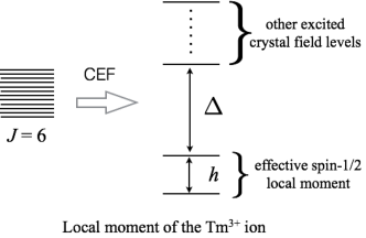
Figure 1: The splitting of the $J=6$ total moment of the Tm³⁺ ion in TmMgGaO₄ under the D_3d crystal electric field (CEF). The energy separation, $h$, between the ground state singlet and the first excited singlet is much smaller than the energy gap, $\Delta$, to the other excited crystal field levels, and the two lowest levels are responsible to the low-temperature magnetic properties.

II Microscopics of $\text{TmMgGaO}{}_{4}$

II.1 Non-degenerate dipole-multipole doublet of Tm³⁺ ion

Properties	non-degenerate DM doublet	DO doublet
original moment	integer	half-odd integer
time reversal	$S^{z}\rightarrow-S^{z}$	$S^{z}\rightarrow-S^{z}$
time reversal	$S^{x,y}\rightarrow S^{x,y}$	$S^{x,y}\rightarrow-S^{x,y}$
degeneracy	two separate singlets	2-fold degenerate
3-fold rotation	eigenvalue $+1$	eigenvalue $-1$

Table 1: The comparison between the non-degenerate dipole-multipole (DM) doublet of the Tm³⁺ ion and the dipole-octupole (DO) doublet for Kramers ions.

Here, for the purpose of completeness, we explain this microscopic physics of the Tm³⁺ ion in the language that is aligned with our early works in the field, and compare it with the well-known dipole-octupole doublet for half-integer moments. The non-degenerate dipole-multipole doublet nature of the Tm³⁺ ion in $\text{TmMgGaO}{}_{4}$ was clarified and carefully modelled in Ref. Shen et al., 2019. The Tm³⁺ ion has a total orbital angular moment ${L=5}$ and total spin moment ${S=1}$, and the spin-orbit coupling gives a total moment ${J=6}$ Shen et al. (2019); Li et al. (2018). The thirteen-fold degeneracy of the total moment is further split by the crystal field. Unlike the usual degeneracy for Kramers doublets and non-Kramers doublet, the ground state and the first excited state of the Tm³⁺ ion are both singlets (see Fig. 1). They are not degenerate, and there is no reason to support the degeneracy of these two states. Each state in the relevant quasi-doublet is an one-dimensional irreducible representation of the D_3d point group, and there should always be a crystal field splitting between two states of the quasi-doublet. This crystal field splitting was further modeled as an intrinsic transverse field by us in Ref. Shen et al., 2019. All these are observed from the form of the wavefunction for each state in the quasi-doublet. The wavefunction is a linear superposition of $|{J^{z}=3n}\rangle$ where $n$ is an integer and $J^{z}$ is defined on the local 3-fold rotational axis of the triangular lattice. In terms of the notation in Ref. Shen et al., 2019, the two wavefunctions are

$$|\Psi_{g}\rangle = c_{6}[|{6}\rangle+|{-6}\rangle]+c_{3}[|{3}\rangle-|{-3}\rangle]+c_{0}\,|{0}\rangle,$$ (1)

$$|\Psi_{e}\rangle = c_{6}^{\prime}[|{6}\rangle-|{-6}\rangle]+c_{3}^{\prime}[|{3}\rangle+|{-3}\rangle],$$ (2)

where $|3n\rangle$ (with $n\in\mathbb{Z}$) refers to the quantum number of $J^{z}$, $|\Psi_{g}\rangle$ ($|\Psi_{e}\rangle$) refers to the ground state (the first excited crystal field level), and the two singlets carry $A_{1g}$ and $A_{2g}$ representation of the $D_{3d}$ point group, respectively. Here $c_{6},c_{3},c_{0},c_{6}^{\prime},c_{3}^{\prime}$ are real numbers with $|c_{6}|\approx|c_{6}^{\prime}|\gg c_{3},c_{3}^{\prime},c_{0}$. Their nature of the one-dimensional irreducible representation can be simply seen by applying the three-fold rotation operation,

$$e^{-i\frac{2\pi}{3}J^{z}}|{J^{z}={3n}}\rangle=|{J^{z}={3n}}\rangle,$$ (3)

other integer spin numbers do not have this property, and they often give rise to two-dimensional representation of the D_3d point group. The point group symmetry does not allow the degeneracy between the ground state singlet and the first excited singlet. Due to the intrinsic integer spin (${J=6}$) in nature for the Tm³⁺ ion, there is no Kramers’ theorem’s protection, either.

It is ready to notice that both $|\Psi_{g}\rangle$ and $|\Psi_{e}\rangle$ are non-magnetic, and thus thinking locally about the single-ion physics would not lead to any magnetism. The magnetism should come from the exchange interaction between the local moments. The intrinsic competition between the single-ion physics and the exchange interaction is captured and modelled as an intrinsic TFIM by us Shen et al. (2019) and will be explained in great details in Sec. III.

As the Tm³⁺ doublet in this context was sometimes referred as a non-Kramers doublet, we here clarify their difference. The usual non-Kramers doublet, that occurs in for example the Pr³⁺ ion Bonville et al. (2016); Chen (2016) of Pr₂Zr₂O₇ and Pr₂Ir₂O₇ or other rare-earth triangular lattice magnets Liu et al. (2018), is composed of two degenerate crystal field states, and their degeneracy is not protected by time reversal but protected by the point group symmetry. These states comprise the two-dimensional irreducible representation of the point group symmetry. In comparison, the Tm³⁺ doublet is two non-degenerate point-group singlets that are two independent one-dimensional irreducible representations.

II.2 Comparison with dipole-octupole doublet

It is instructive to compare the non-degenerate dipole-multipole doublet of the Tm³⁺ ion with the dipole-octupole doublet that also arises from the one-dimensional irreducible representations of the D_3d point group. The dipole-octupole doublet was first introduced in the context of pyrochlore magnets in Refs. Huang et al., 2014; Li and Chen, 2017 and then extended to the triangular lattice magnets in Refs. Li et al., 2016a, b; Liu et al., 2018. The dipole-octupole doublet was found to be applicable to the Nd³⁺ ion in various Nd-based pyrochlores Lhotel et al. (2015); Anand et al. (2015); Bertin et al. (2015); Xu et al. (2015); Hatnean et al. (2015); Petit et al. (2016); Benton (2016); Dalmas de Réotier et al. (2017), the Sm³⁺ ion in Sm₂Ti₂O₇ Mauws et al. (2018); Pe çanha Antonio et al. (2019), the Ce³⁺ ion in Ce₂Sn₂O₇ Sibille et al. (2015, 2019); Li and Chen (2017) and Ce₂Zr₂O₇ Gaudet et al. (2019); Gao et al. (2019); Yao et al. (2020), and the Er³⁺ ion in the spinel compounds Lago et al. (2010); Gao et al. (2018). In fact, the dipole-octupole doublet can broadly exist in magnets whose local environment has a D_3d point group symmetry. In this regards, other lattice geometry such as honeycomb magnet could support the dipole-octupole doublet Liu et al. . As a parallel thought, the Tm³⁺ dipole-multipole doublet could broadly exist in many other structures. This is discussed in some details in Sec. VIII.

For the dipole-octupole doublet, the wavefunction of each state in the doublet is a linear superposition of $|{J^{z}=3n/2}\rangle$ where $n$ is an odd integer and $J^{z}$ is defined on the local 3-fold rotational axis. On the triangular lattice, the local 3-fold rotational axis aligns with the global $z$ axis, while it is not the case for the pyrochlore lattice. The reason that it is a one-dimensional irreducible representation can be seen by applying the three-fold rotation operation,

$$e^{-i\frac{2\pi}{3}J^{z}}|{J^{z}=\frac{3n}{2}}\rangle=-|{J^{z}=\frac{3n}{2}}\rangle.$$ (4)

The eigenvalue of the 3-fold rotation is $-1$, instead of $+1$ for the dipole-multipole doublet of the Tm³⁺ ion. Unlike the non-degenerate dipole-multipole doublet of the Tm³⁺ ion, the dipole-octupole doublet for the Kramers ion is degenerate, and the degeneracy is protected by the time reversal symmetry due to the Kramers’ theorem for the half-integer spin moment.

III Effective model of $\text{TmMgGaO}{}_{4}$

Figure 2: (a) Definition of the triangular lattice. The three sublattices are marked by blue, red and black colors, respectively. (b) The Brillouin zone of triangular lattice.

Like any two-level systems, the Tm³⁺ doublet can be captured by an effective spin-1/2 operators that operate on the manifold of the doublet. We define the following effective spin-1/2 operator $\boldsymbol{S}_{i}$ on each Tm site,

$$S_{i}^{x} =\frac{i}{2}\left(|\Psi_{i,e}\rangle\langle\Psi_{i,g}|-|\Psi_{i,g}\rangle\langle\Psi_{i,e}|\right),$$ (5)

$$S_{i}^{y} =\frac{1}{2}\left(|\Psi_{i,g}\rangle\langle\Psi_{i,g}|-|\Psi_{i,e}\rangle\langle\Psi_{i,e}|\right),$$ (6)

$$S_{i}^{z} =\frac{1}{2}\left(|\Psi_{i,g}\rangle\langle\Psi_{i,e}|+|\Psi_{i,e}\rangle\langle\Psi_{i,g}|\right).$$ (7)

We can see from the effective spin definition that $|\Psi_{i}^{\pm}\rangle$ are eigenstates of $S^{y}$ with eigenvalue ${S^{y}=\pm 1/2}$, while the $S^{x}$ and $S^{z}$ components introduces hybridization between $|\Psi_{i}^{\pm}\rangle$. From our definition of the spin operators, the point group symmetry demanded splitting between $|\Psi_{i,g}\rangle$ and $|\Psi_{i,e}\rangle$ is modelled as an intrinsic transverse field on the $y$ component of the effective spin, i.e. $-h\sum_{i}S_{i}^{y}$, where $h$ is the crystal electric field splitting. Moreover, the “$x$” and “$y$” in $S^{x}$ and $S^{y}$ are defined in the internal Hilbert space of the crystal field states, $|\Psi_{i,g}\rangle$ and $|\Psi_{i,e}\rangle$, and have no connection to the real space. However, we often refer these two components as “in-plane components” for convenience. The $S^{z}$ component has its physical meaning both for the real space and for the internal Hilbert space.

It is illuminating to obtain the symmetry properties of the effective spin operators. Under the point group symmetry and the time reversal (${\mathcal{T}}$) operations, the effective spin components transform as,

$$C_{3}: \quad S_{i}^{x}\rightarrow+S_{i}^{x},S_{i}^{y}\rightarrow S_{i}^{y},S_{i}^{z}\rightarrow+S_{i}^{z},$$ (8)

$$C_{2}^{\prime}: \quad S_{i}^{x}\rightarrow-S_{i}^{x},S_{i}^{y}\rightarrow S_{i}^{y},S_{i}^{z}\rightarrow-S_{i}^{z},$$ (9)

$${\mathcal{T}}: \quad S_{i}^{x}\rightarrow+S_{i}^{x},S_{i}^{y}\rightarrow S_{i}^{y},S_{i}^{z}\rightarrow-S_{i}^{z},$$ (10)

where $C_{3}$ refers to three-fold rotation about c axis, $C_{2}^{\prime}$ refers to two-fold rotation along the bond direction. The in-plane component $S^{x}$ and $S^{y}$ operators are time reversal even and transform as even-order multipole moments under crystal symmetries. From the wavefunction of $|\Psi_{g}\rangle$ and $|\Psi_{e}\rangle$, it is clear that $S^{x}$ and $S^{y}$ mostly connect $|{J^{z}=6}\rangle$ and $|{J^{z}=-6}\rangle$ and are mostly involve the 12th order multipole moments. The $S^{z}$ component is odd under time reversal and transforms as dipole moment. The low-temperature magnetization is provided by $\langle\sum_{i}S_{i}^{z}\rangle$. While the dipole moment, $S^{z}$, can be probed by neutron scattering, the multipole moments are hidden or invisible in most conventional experimental probes and are often referred as “hidden orders” or “hidden components” in the literature.

Based on the saturated values of the magnetic moment in the field, one can infer that the Tm local moment is almost an Ising spin. This is also understood from the wavefunctions of $|\Psi_{g}\rangle$ and $|\Psi_{e}\rangle$ where $|{J^{z}=\pm 6}\rangle$ are dominant. The exchange interaction between the Tm local moments would be primarily an Ising interactions. The exchange interaction between the transverse components are strongly suppressed as $S^{x}$ and $S^{y}$ are high order multipole moments and they are even higher than the quadrupole moments. The resulting effective Hamiltonian for the interacting Tm local moment is the TFIM

$$H=\sum_{\langle ij\rangle}J_{zz}S_{i}^{z}S_{j}^{z}-\sum_{i}\left(hS_{i}^{y}+BS_{i}^{z}\right),$$ (11)

where ${B\equiv\mu_{B}g_{\parallel}B^{z}}$ represents the external magnetic field along the $z$ direction, and $h$ is the intrinsic transverse field. In Ref. Shen et al., 2019, we actually included a tiny second neighbor Ising interaction $J_{2}$ to improve the fitting to the experiments. As the interaction energy scale between the Tm local moment is already quite small, the tiny $J_{2}$ does not change the qualitative physics in this paper. Thus, we will rely on the above minimal model to capture the essential physics about TmMgGaO₄ and other intrinsic quantum Ising magnets. Nevertheless, if one is more interested in the quantitative aspects, other non-essential and non-universal ingredients should be included into our Hamiltonian. These would involve the long-range dipole-dipole ($S^{z}$-$S^{z}$) interaction and the van-Vleck process through the excited crystal field states.

The magnetic moment of the Tm³⁺ ion is much larger than the one for the Yb³⁺ ion in YbMgGaO₄. Although the first-neighbor dipole-dipole interaction may be incorporated with the superexchange interaction and modelled as a total $J_{zz}$ interaction, we here estimate the further neighbor dipole-dipole interaction and find that the second-neighbor dipole-dipole interaction is 0.48K, the third-neighbor dipole-dipole interaction is 0.31K, the fourth-neighbor dipole-dipole interaction is 0.134K, the fifth-neighbor dipole-dipole interaction is 0.092K, and the sixth-neighbor dipole-dipole interaction is 0.053K. If one simply attributes all the further neighbor interactions beyond the first neighbor to the dipole-dipole interactions, one readily finds from the Curie-Weiss temperature ($-19$K) Shen et al. (2019) that the first neighbor interaction $J_{zz}$ is ${\sim 11.5}$K and should dominate over further neighbor interactions. Thus, it is legitimate for us to keep only the first neighbor or first few neighbor interations in TRIM to capture the qualitative physics. Moreover, the energy gap from the doublet to the lowest crystal field excited level is smaller than the one in YbMgGaO₄ . Thus the virtual van-Vleck process could further bring extra ingredients into the quantitative modelling.

IV Qualitative understanding from experiments

While the intrinsic quantum Ising model for TmMgGaO₄ was derived from the microscopics in Sec. III and in Ref. Shen et al., 2019, various physical insights can be gained from the careful reading of the existing experiments before the derivation and solving of this model. To the best of our knowledge, the single crystal sample of TmMgGaO₄ and its basic structure and thermodynamic properties were reported in Ref. Cevallos et al., 2018. Even though the measurements were performed above 1.8K, the magnetization results already show the strong Ising-like features. More low-temperature thermodynamic measurements were obtained in Ref. Li et al., 2018, and the results were interpreted from classical Ising moments with competing Ising interactions. The low-temperature magnetic state was suggested to be a stripe order with an alternating Ising spin arrangement on two magnetic sublattices, and the transition to the stripe order was suggested to occur at $\sim 0.27$ K. This spin state has an ordering wavevector at the momentum point $M$ in the Brillouin zone. The detailed elastic and inelastic neutron scattering measurements were performed in Ref. Shen et al., 2019 together with the low-temperature thermodynamic measurements. The appearance of the magnetic Bragg peak at the wavevector $K$ coincides with the peak at $\sim 1$ K in the specific heat data. The ordering wavevector $K$ indicates a three-sublattice magnetic order structure, which differs from the proposal of stripe order in Ref. Li et al., 2018. Moreover, the data-rich inelastic neutron scattering measurements show a coherent spin-wave like excitation spectrum with a well-defined dispersion.

The first question is, what does neutron scattering measurement actually detect? This question is also useful in our actual calculation of the physical properties. There are two ways to think about this. The first way is to rely on experiments, i.e., using experiments to understand experiments. The magnetization measurements suggest that the in-plane components of the local moment, if they exist, almost do not respond to the application of the external magnetic field. The neutron spin couples to the local moment in the same way as the external magnetic field would do. The neutron spin naturally picks up the out-of-plane component, $S^{z}$, of the local moment. Thus, the magnetic Bragg peak at the $K$ point indicates a three-sublattice structure for the $S^{z}$ components. Likewise, the inelastic neutron scattering detects the dynamic part of the $S^{z}$-$S^{z}$ correlator, even though it is a regular neutron scattering measurement and functions as a polarized neutron scattering. The second way is based on the microscopics. Microscopic analysis tells us that, the out-of-plane component, $S^{z}$, is a magnetic dipole moment, and couples linearly with the external magnetic field, while the in-plane components, $S^{x,y}$, are the magnetic multipole moments and do not couple to the magnetic field at the linear order. The coupling of $S^{x,y}$ to the field could occur at high orders but is suppressed due to the large crystal field energy separation between the non-degenerate dipole-multipole doublet and the other highly excited crystal field levels. Knowing the microscopic facts, one can immediately conclude that the neutron scattering measurement detects the properties of the $S^{z}$ component.

The next level of question is how to reconcile these experiments. Again, we first rely on the experiments and then turn to the microscopics. Let us start with the first possibility. If the Tm³⁺ local moment is truly Ising spin with Ising interaction like the one used in Ref. Li et al., 2018, then there is no quantum mechanics, and there should not be any dispersion-like excitation. It is not the case in the inelastic neutron measurement in Ref. Shen et al., 2019. The second possibility is that the local moment is a quantum spin and all the three components are present and active in the physical Hilbert space. From the elastic neutron scattering measurement, we can conclude that, the $S^{z}$ component has ${\langle S^{z}\rangle\neq 0}$ and develops a three-sublattice structure at low temperatures, but we do not know anything about the in-plane components $S^{x}$ and $S^{y}$. If ${\langle S^{x}\rangle=\langle S^{y}\rangle=0}$, then the dynamic correlation of $S^{z}$-$S^{z}$, that is detected by the inelastic neutron scattering measurement, would simply be a two-magnon continuum. This is again not the case in the experiments. Thus, we expect that, at least one component of the in-plane components should be non-zero, even though they are not experimentally visible. The role of the $S^{z}$ operator is to flip the in-plane component and create a coherent magnetic excitation. To summarize this part of reasoning, we conclude from reading the experiments with an intertwined dipolar and multipolar orders for the ground state of TmMgGaO₄,

$$\langle S^{z}\rangle\neq 0\text{\quad with a three-sublattice structure},$$ (12)

$$\langle S^{x}\rangle\neq 0\text{\quad and/or \quad}\langle S^{y}\rangle\neq 0.$$ (13)

From the microscopics and our modeling, it is obvious to see that the invisible component, $S^{y}$, is non-zero as it is polarized by the intrinsic transverse field.

The final issue to resolve is to see whether our microscopic modeling can provide useful understanding of the physical properties and insights for future experiments on TmMgGaO₄ and/or other Tm-based triangular lattice magnets. This is carried out in the next few sections.

V Phase diagram

V.1 Mean-field analysis

The TFIM on the triangular lattice has been well-studied in the absence of the external magnetic field Moessner and Sondhi (2001); Isakov and Moessner (2003), while the situation with the longitudinal field has not been investigated yet. To gain some physical insight into the ground state phase diagram, we first tackle with the Weiss mean-field approximation by decoupling interactions between different spins as

$$S_{i}^{z}S_{j}^{z}\rightarrow\langle S_{i}^{z}\rangle S_{j}^{z}+S_{i}^{z}\langle S_{j}^{z}\rangle-\langle S_{i}^{z}\rangle\langle S_{j}^{z}\rangle.$$ (14)

Here the mean-field order parameter $\langle S_{i}^{z}\rangle$ needs to be solved self-consistently. The mean-field phase diagram is depicted in Fig. 3(a).

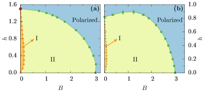
Figure 3: Phase diagram of the model in Eq. (11). Here we set the energy unit ${J_{zz}=1}$. Two three-sublattice ordered phases, I (orange) and II (green) and a polarized phase are found in the phase diagram. The red dot represents quantum phase transition with (2+1)d XY universality class. The left (a) is the mean-field result, and the right (b) is the Monte Carlo result that is calculated at inverse temperature $\beta=8L$ with system sizes $N=L\times L$ $(L=6,12,24)$. The phase boundary from phase I to II is difficult to be captured in the current algorithm and are schematic here.

In the Ising limit (without the transverse and longitudinal fields), the system lies at a classically critical state that hosts a macroscopic ground-state degeneracy: any spin configuration with “2-up-1-down” or “1-up-2-down” has the minimal energy. With introducing the transverse field $h$, quantum fluctuations allow quantum tunneling within the massively degenerate manifold. This quantum tunneling lifts the macroscopic degeneracies and eventually stabilizes a three-sublattice long-range ordered phase (dubbed the three-sublattice “I” state) as the ground state owing to the quantum order-by-disorder mechanism. Since the three-sublattice ordering is entirely contributed by the quantum fluctuations, it is relatively weak and is controlled by quantum fluctuation $h$ in a non-monotonic fashion: with $h$ being too small the quantum order-by-disorder effect is weak, while for a very large $h$ the polarization effect becomes more important, suppresses the three-sublattice ordering and drives the system into the “quantum disordered” state where the spins are fully polarized along the transverse direction. Although the above results are obtained mean-field level, they are consistent with those obtained via quantum dimer model mapping where quantum fluctuations are taken into account in a perturbative manner Moessner et al. (2000); Moessner and Sondhi (2001).

As the external longitudinal field $B$ is applied at the Ising limit, the system immediately becomes unstable against the magnetic ordering due to the criticality at this point. The resulting state is another three-sublattice ordered state called “1/3-plateau” state with a “2-up-1-down” structure on each triangular plaquette. Unlike the pure quantum origin in the “I” phase, the three-sublattice ordering of the plateau state arises at the classical level and are more stable. The plateau state remains as the ground state upon increasing the magnetic field until the system becomes fully polarized at ${B_{c}=3J_{zz}}$ through a first-order transition. When the quantum fluctuation $h$ is switched on, the three-sublattice “plateau” state becomes the “quasi-plateau” phase (dubbed three-sublattice “II” state) because the total magnetization is no longer a good quantum number. Moreover, as the three-sublattice “I” phase is generated by the quantum fluctuations and is fully gapped, it is stable against the weak perturbations. But since that the ordering is rather weak, a small external field $B$ could drive the system to the quasi-plateau state across a phase transition. The transition from “I” to “II” state is of the second-order, while the transition from “II” to the fully polarized state is of the first-order, consistent with what happens at ${h=0}$ limit. The two phase boundaries terminate at the classical critical point ${h=0}$, and at the quantum critical point ${h_{c}^{\textrm{MF}}=1.5J_{zz}}$, both located along ${B=0}$ axis. These are depicted in Fig. 3(a) and obtained from the mean-field analysis.

V.2 Path-integral quantum Monte Carlo method

To examine our mean-field results, we perform the quantum Monte Carlo (QMC) simulations. We choose the the path-integral with the $\{S_{i}^{z}\}$ basis. The partition function of the original model is mapped onto a worldline representation:

$${\mathcal{Z}} = \text{Tr}\left[e^{-\beta\mathcal{H}}\right]=\sum\limits_{\{\alpha_{0}\}}\langle\alpha_{0}|e^{-\beta\mathcal{H}}|\alpha_{0}\rangle$$ (15)

$$= \lim_{{\scriptstyle{{d\tau=\frac{\beta}{n}}\atop{\scriptstyle{n\rightarrow\infty}}}}}\sum\limits_{{\scriptstyle{{\{\alpha\}}\atop{\scriptstyle{\alpha_{n}=\alpha_{0}}}}}}\langle\alpha_{n}|e^{-\mathcal{H}d\tau}|\alpha_{n-1}\rangle\cdots\langle\alpha_{1}|e^{-\mathcal{H}d\tau}|\alpha_{0}\rangle$$

$$= \sum\limits_{\{\alpha\}}\sum_{k=0}^{\infty}\int_{0}^{\beta}\cdot\cdot\int_{\tau_{{}_{2k-1}}}^{\beta}\prod_{i=1}^{2k}d\tau_{i}\ h^{2k}e^{{-\int_{0}^{\beta}U(\tau)d\tau}},$$

where

$$U(\tau)=\langle\alpha(\tau)|\left(\sum_{\langle ij\rangle}J_{zz}S_{i}^{z}S_{j}^{z}-\sum_{i}BS_{i}^{z}\right)|\alpha(\tau)\rangle.$$ (16)

In Fig. 4(a), we depict a representative worldline configuration that contributes to the partition function. The transverse field term of $\sum_{i}hS_{i}^{y}$ causes the spin $S^{z}$ to flip, and we refer such a flipping event as a kink. The temporal periodic boundary condition ${|\alpha(0)\rangle=|\alpha(\beta)\rangle}$ of the path integral demands the number of the kinks $N_{k}$ to be even with ${N_{k}=2k}$ ($k\in\mathbb{Z}$) in Eq. (15). Due to the presence of the longitudinal field $B$, the cluster update fails, and instead, we design a metropolis algorithm that contains two update schemes, creation/deletion flat and shift kink, as shown in Fig. 4. The calculations of acceptance rates of update schemes are quite standard through the detailed balance equation, and we will not show them explicitly here. The thermal annealing procedure is employed to deal with the freezing issue of the Monte Carlo simulation.

In the QMC simulations, we take the system sizes $N=L\times L$ $(L=6,12,24)$ with periodic boundary condition. The ground-state phase diagram is calculated at inverse temperature $\beta=8L$ and the result is shown in Fig. 3(b) through the finite size scaling. The QMC phase diagram agrees with the mean-field one at the qualitative level. The locations of the phase boundaries differ quantitatively. The critical field ${h_{c}^{\textrm{MC}}\approx 0.82J_{zz}}$ Isakov and Moessner (2003); Wang et al. (2017) is almost half of the mean-field result ${h_{c}^{\textrm{MF}}=1.5J_{zz}}$ with zero external field ${B=0}$. This is as expected, as the mean-field approximation underestimates the quantum fluctuations especially for the phase boundaries. Nevertheless, the mean-field theory provides the essential physical understanding and insights for the magnetic properties of the system.

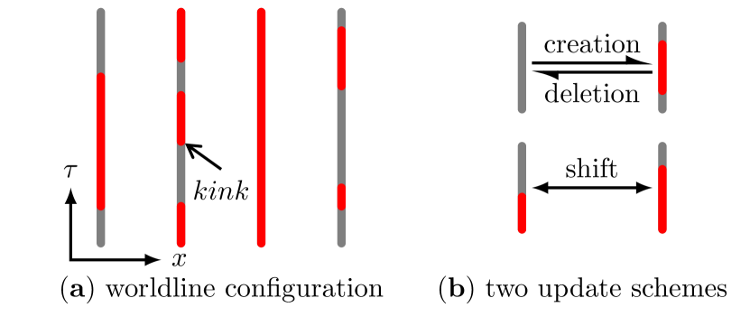
Figure 4: The worldline configuration under imaginary time evolution and update schemes. (a) is a worldline configuration of four spins in a chain. Different colors correspond to different spin $S^{z}$ states. Along the imaginary time, every spin worldline may be divided into several flats by cause of $S_{i}^{y}$. (b) the diagrammatic sketch of the update schemes.

V.3 Finite temperature regimes and BKT transitions

In this subsection, we extend the analysis from the zero temperature or the near-ground-state low temperatures to finite temperatures and study the finite temperature properties and the phase transitions out of the ordered one. To reveal the finite-temperature transitions, it is necessary to perform the field theoretical analysis near the transition and then supplement with the QMC calculations. The three-sublattice order parameter is characterized by the Fourier transformed $S^{z}$ dipolar component at the $K$ point. This can be captured by the following complex field

$$\psi=\frac{1}{\sqrt{3}}(m_{1}+m_{2}e^{i2\pi/3}+m_{3}e^{-i2\pi/3}),$$ (17)

where $m_{i}$ (${i=1,2,3}$) are the dipolar magnetizations of the three sublattices at the neighboring sites, and we have set the lattice constant to unity. We can see that $\psi$ characterizes the three-sublattice ordering, as ${\psi=0}$ occurs only when ${m_{1}=m_{2}=m_{3}}$, where the three-sublattice order vanishes. The transformation of the field variable $\psi$ under the lattice translation $T_{\hat{x}}$ and the time reversal ${\mathcal{T}}$ operation take the following form

$$T_{\hat{x}}: \psi\rightarrow\psi e^{i2\pi/3},$$ (18)

$${\mathcal{T}}: \psi\rightarrow-\psi.$$ (19)

For the three-sublattice “I” state, the spin alignments at the three sublattices are different from one another, therefore the ground state is six-fold degenerate. With zero external magnetic field, the $\psi$ corresponding to the ground states are located at a circle in the complex plane with $\mathrm{Arg}\,\psi=(2n+1)\pi/6$ $(n=0,1,...,5)$ that are protected by the translation and time-reversal symmetry (see Fig. 5(a)). This clock anisotropy is robust against the short-range interactions such as weak transverse exchange and next-nearest-neighbor Ising interactions that are present in the materials, therefore our analysis remains valid against these perturbations. In the vicinity of the melting of the magnetic order, the coarse-grained Landau-Ginzburg-Wilson free energy dictates the $\mathbb{Z}_{6}$ clock anisotropy takes the following form Blankschtein et al. (1984)

$$H_{\textrm{LGW}}= -K|\nabla\psi|^{2}+r\psi^{*}\psi+u_{4}(\psi^{*}\psi)^{2}+u_{6}(\psi^{*}\psi)^{3}$$

$$+v_{6}(\psi{}^{6}+\psi^{*}{}^{6})$$ (20)

with ${\psi=|\psi|e^{i\theta}}$, where $\theta$ corresponds to the phase of the field $\psi$. The $\mathbb{Z}_{6}$ clock anisotropy term $v_{6}$ has a significant implication on the nature of thermal and quantum phase transitions. First of all, let us examine the thermal melting of the three-sublattice states. Since the clock anisotropy term is brought about by the quantum fluctuations from the transverse field and is expected to be small, the phase fluctuations of the order parameter $\psi$ is soft therefore becomes important for the thermal melting at the first stage. By integrating out the amplitude fluctuations, we obtain the 2D XY model with a $\mathbb{Z}_{6}$ clock anisotropy. This theory exhibits an approximate self-duality Chen et al. (2017); Ortiz et al. (2012), where the dual theory is described in terms of vortices of $\theta$ that acts as the disorder parameter of the original theory. It was previously understood that, certain self-dual quantum critical points can put constraints on the physical observables such as a non-divergent Grüneisen ratio Zhang (2019). The current transition is an approximate self-duality and is driven by temperature. Whether an analogous property can occur here will be explored in future work.

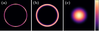
Figure 5: Histograms of the order parameter $\psi$ in different temperature regimes obtained from QMC simulations. (a): three-sublattice long-range ordered state at low temperature ${T=0.025}$. (b): quasi-long-range ordered “BKT phase” at intermediate temperature ${T=0.075}$. (c): disordered state at high temperature ${T=0.225}$. In the QMC simulations we set the model parameter ${J_{zz}=1}$, ${h=0.4}$, ${B=0}$ and the system size ${L=12}$.

The thermal melting of the three-sublattice order takes a two-step manner Biswas and Damle (2018); Damle (2015); Moessner et al. (2000); Isakov and Moessner (2003) and is also clearly identified in the order parameter histogram as is shown in Fig. 5. At the low-temperature phase ${T<T_{c1}}$ that is proximate to the ground state, the $\mathbb{Z}_{6}$ clock term is relevant such that the phase of $\phi$ is pinned to six equivalent angles, and we have the three-sublattice long-range ordered state. This can be seen in the angular histogram plot of the order parameter $\psi$ in Fig. 5(a) where the six-fold variation is shown. The dual phase at ${T>T_{c2}}$ is the high-temperature disordered phase where the vortices proliferate. The higher temperature transition at $T_{c2}$ belongs to the BKT universality class, while the lower temperature transition at $T_{c1}$ is dual to the high temperature one and hence is called the “inverse BKT” transition. Unlike the 2d XY model with a global U(1) symmetry where $T_{c1}$ and $T_{c2}$ coincide, in our case $T_{c1}$ and $T_{c2}$ do not coincide due to the presence of ${\mathbb{Z}}_{6}$ clock term in the free energy of Eq. (20). In the intermediate temperature ${T_{c1}<T<T_{c2}}$ we have an extended phase where both vortices and the clock anisotropy become irrelevant. The irrelevance of clock anisotropy indicates an emergent continuous U(1) symmetry that is shown in Fig. 5(b). Due to the emergent U(1) symmetry, the system behaves just like the low-temperature quasi-long-range ordered phase of the XY model without any anisotropy term and supports an algebraic spin correlation, and this thermal regime with ${T_{c1}<T<T_{c2}}$ is referred to as BKT phase Biswas and Damle (2018); Damle (2015); Moessner et al. (2000). As long as the ground state is in the three-sublattice ordered phase, this BKT phase generically occurs in the finite temperature regime regardless of the parameters. For this reason, we plot the finite temperature phase diagram in Fig. 6 with a single choice of transverse field ${h/J\approx 0.65}$ that might be appropriate for TmMgGaO₄ inside the three-sublattice ordered phase.

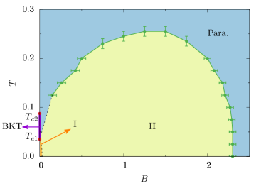
Figure 6: Finite temperature phase diagram with an external magnetic field $B$ obtained from QMC simulations. The parameter we take is $J_{zz}=1$, $h=0.65$ where the ground state is a three-sublattice ordered state. The “BKT phase” at $B=0$ axis is marked by thick purple line. The lower and upper BKT transition points are $T_{c2}=0.09(2)J_{zz}$ and $T_{c1}=0.035(15)J_{zz}$ Isakov and Moessner (2003). The green solid-dot line refers to first-order transition while the upper and lower red dots at $B=0$ axis correspond to BKT and inverted BKT transitions, respectively. The phase boundaries (dash lines), when $B$ is very small, are difficult to be captured in the current algorithm and are schematic here. The QMC simulation is performed with system sizes $L=6,12,24$ with the periodic boundary condition.

The underlying reason for the finite-temperature BKT physics in this context arises from the emergent U(1) symmetry. This emergent U(1) symmetry, however, no longer holds in the presence of external magnetic fields. The magnetic field breaks the time-reversal symmetry and brings about a $\mathbb{Z}_{3}$ clock anisotropy to the system Damle (2015),

$$H_{3}=v_{3}(\psi{}^{3}+\psi^{*}{}^{3}),$$ (21)

with $v_{3}$ linearly proportional to $B$. This $\mathbb{Z}_{3}$ clock term is always relevant at the phase transition. Therefore, the successive BKT transition scenario in thermal melting as well as an emergent continuous symmetry are no longer presented. Moreover, from Eq. (20) and Eq. (21) we obtain the order parameter symmetry for each phases, as is shown in Fig. 7. We find that with magnetic field the order parameter symmetry of the three-sublattice “I” is reduced from $\mathbb{Z}_{6}$ to $\mathbb{Z}_{3}\times\mathbb{Z}_{2}$. The symmetry is further reduced to $\mathbb{Z}_{3}$ in the intermediate three-sublattice “II” state.

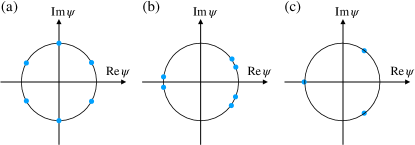
Figure 7: Evolution of the order parameter manifold (marked as blue dots) with external magnetic field $B$. (a): the “I” state with $B=0$; (b) the “I” state with small $B\neq 0$; (c): the intermediate three-sublattice “II” state with larger $B$. The the symmetry of order parameter manifolds are $\mathbb{Z}_{6}$, $\mathbb{Z}_{3}\times\mathbb{Z}_{2}$ and $\mathbb{Z}_{3}$ for three cases, respectively.

The finite-temperature phase diagram of the three-sublattice state is shown in Fig. 6. According to Fig. 6, if one lowers the temperature from the trivial high-temperature paramagnetic phase at ${B=0}$, one experiences two successive transitions at $T_{c2}$ and $T_{c1}$. For BKT transitions the correlation length diverges too fast near the thermal transition, the diverging behavior of the specific heat near the transition temperatures cannot be very well observed experimentally or even numerically. This seems to be what happens for TmMgGaO₄: no diverging behavior is revealed in the specific heat data, instead only tiny anomaly with a slightly broad peak is shown at ${\sim 1}$K Li et al. (2018); Shen et al. (2019).

With magnetic field in Fig. 6, the $\mathbb{Z}_{3}$ clock anisotropy is introduced and the BKT scenario breaks down. For the intermediate “II” state that breaks $\mathbb{Z}_{3}$ symmetry, there is only the first order thermal transition. For the “I” state that breaks $\mathbb{Z}_{2}$ symmetry in addition to $\mathbb{Z}_{3}$, the $\mathbb{Z}_{2}$ and $\mathbb{Z}_{3}$ symmetries should break at different temperatures, therefore one expects another Ising transition in addition to the first order transition in the thermal melting. Unlike the BKT transitions that are weak and unclear in the heat capacity, these transitions are expected to show diverging signals (the Ising transition) or discontinuous signals (the first order transition) in the thermodynamic measurements, as is shown in the magnetic specific heat data in Ref. Li et al., 2018. However, for the transitions involving the “I” state where the magnetic field is weak, the divergent behavior is too weak to be observed experimentally or even numerically, as the system is close to the $B=0$ point where the BKT scenario happens.

V.4 Some experimental implications on BKT physics

Experimentally, it is typically hard to detect BKT transitions in magnetic systems. Here we discuss how to determine BKT transition temperatures from experiments. Inside the BKT phase between $T_{c2}$ and $T_{c1}$, the algebraic spin correlation would lead to quasi-Bragg peak at the wavevector $K$. In principle, Bragg peaks may be distinguished from quasi-Bragg peaks by the elastic peak profile at the $K$ point, but this is again difficult. Further neutron scattering studies might be useful to sort out the lower transition temperature $T_{c1}$.

A relevant experimental prediction given by K. Damle in Ref. Damle, 2015 is the singular uniform magnetic susceptibility along $z$ direction in part of the BKT phase regime, despite absence of ferromagnetic order in this system. Due to the small energy scale of the interaction, the direct susceptibility measurements may not be able to give clear signals especially because the impurity and disorder effects could affect very low-temperature thermodynamic behaviors. Somewhat equivalently, it is more convenient for us to examine the $S^{z}$-$S^{z}$ correlation at the $\Gamma$ point in the neutron scattering measurement. From the available neutron data for TmMgGaO₄ Shen et al. (2019), we observe a clear upturn of the Bragg peak intensity below $\sim 1$ K. This $\Gamma$ point upturn at $\sim 1$K may be interpreted as the onset of the BKT phase if this upturn is not due to any other reason. Thus we identify $T_{c2}$ as $\sim 1$K, that is consistent with the $T_{c2}$ obtained from the magnetic specific heat. From the phase diagram by Isakov and Moessner in Ref. Isakov and Moessner, 2003 that indicated the phase boundary of the BKT phase, we conclude that $T_{c1}$ is $\sim 0.5$K. Thus, we postulate that the range of BKT phase is from $\sim 0.5$K to $\sim 1$K for TmMgGaO₄.

Here we numerically examine the power-law behaviors of the $S^{z}$-$S^{z}$ correlation at $\Gamma$ point and at $K$ point inside the BKT phase. We have

$$\chi_{{}_{\Gamma}}=\frac{L^{2}}{\beta}\Big{\langle}\Big{|}\int_{0}^{\beta}d\tau\ m_{{}_{\Gamma}}(\tau)\Big{|}^{2}\Big{\rangle},$$ (22)

and the order parameter susceptibility

$$\chi_{{}_{K}}=\frac{L^{2}}{\beta}\Big{\langle}\Big{|}\int_{0}^{\beta}d\tau\ m_{{}_{K}}(\tau)\Big{|}^{2}\Big{\rangle},$$ (23)

where ${m_{\bf q}\equiv\frac{1}{N}\sum_{i}S_{i}^{z}\exp(i{\bf q}\cdot{\bf r}_{i})}$ with $N$ the system size. According to the previous field theoretical analysis by K. Damle Damle (2015), they are expected to scale with the system size $L$ as

$$\chi_{{}_{\Gamma}}\sim L^{2-9\eta(T)},$$ (24)

$$\chi_{{}_{K}}\sim L^{2-\eta(T)},$$ (25)

with ${1/9\leq\eta(T)\leq 2/9}$ in part of the BKT phase Damle (2015). The QMC results are shown in Fig. 8 and both fit rather well to Eq. (24) and Eq. (25). Although there is always no ferromagnetic long-range order in the BKT phase, $\chi_{{}_{\Gamma}}$ is still divergent with the system size in part of the phase region.

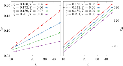
Figure 8: Susceptibilities $\chi_{{}_{\Gamma}}$ and $\chi_{{}_{K}}$ versus the linear system size $L$ for four different temperatures when $h=0.65$ in BKT phase. Solid lines are power-law forms $\sim L^{2-9\eta}$ (on the left panel) and $\sim L^{2-\eta}$ (on the right panel). Small systems maybe will deviate from power-law forms due to the effect of large-finite size scaling.

VI Dynamic properties from orthogonal operator approach and selective measurements

The previous section deals with the phase diagram and the magnetic ordering structures. These properties are static magnetic properties. To provide more information about the system, we here explore the dynamic properties from the orthogonal operator approach and the selective measurements. In Sec. VI.1, we explain the “orthogonal operator approach”. In Sec. VI.2, we turn to the selective measurement that directly applies the “orthogonal operator approach” for the Tm-based triangular lattice antiferromagnets.

VI.1 Orthogonal operator approach

Even though the in-plane components are non-zero, they are not visible from the experiments. These “hidden order”-like features can be revealed from an approach called “orthogonal operator approach” Liu et al. (2018); Li et al. (2016a). The notion of “hidden order” was introduced into condensed matter physics in the study of the compound URu₂Si₂ Mydosh and Oppeneer (2014). The order parameter associated with the hidden order does not couple strongly with the conventional experimental probe such that the order does not explicitly show up in the usual experimental probes. To identify the nature of the hidden order, our simple suggestion was to find the physical observables whose operators do not commute with the proposed hidden order operators, and at the same time make sure these observables are ready to detect experimentally. These operators are referred as “orthogonal operators”. The dynamic correlations or spectra of these operators would reveal the structure and the nature of the underlying hidden orders. These thoughts have been explored for the quadrupolar orders and the octupolar orders of triangular lattice magnets Liu et al. (2018); Li et al. (2016a) as well as the spin nematics in frustrated magnets Smerald and Shannon (2013).

Because the non-vanishing in-plane components are induced by the intrinsic transverse field, strictly speaking, they are not the Landau symmetry breaking orders. Nevertheless, their presence and behavior are very much similar to the roles of the hidden orders and thus can be understood in a similar manner.

VI.2 Selective measurements

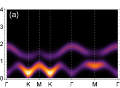
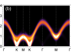
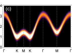
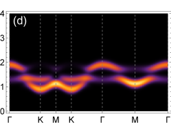
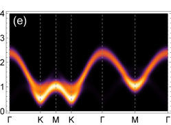
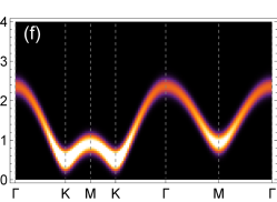
Figure 9: Dynamical correlation function $\mathcal{S}^{zz}(\boldsymbol{q},\omega)$ calculated within the linear spin-wave theory of (a),(b):the three-sublattice “I” state, (c),(d): the intermediate three-sublattice “II” state and (c),(f): the paramagnetic (or polarized) state. The parameter we take for the representative points are (a): ${h=0.8}$, ${B=0}$; (b): ${h=1.3}$, ${B=0}$; (c): ${h=2}$, ${B=0}$, (d): ${h=0.8}$, ${B=1.3}$; (e): ${h=1.3}$, ${B=1.3}$; (f): ${h=1.3}$, ${B=1.8}$. In all cases we take ${J_{zz}=1}$.

Having figured out the phase diagrams in the previous section, we here explain the experimental consequences for the dynamics from the selective measurements and the orthogonal operator approach. The three-sublattice order that we found from the model is characterized by the order parameter $\psi$ defined by the dipolar magnetization, which is directly reflected as the magnetic Bragg peaks at the $K$ point. Meanwhile, due to the intrinsic crystal field, there is always a non-vanishing expectation value in the transverse components that arises not from the spontaneous symmetry breaking but from the intrinsic polarization effect. Since the transverse components are the magnetic multipoles, they do not directly couple to the neutron spins hence are hidden in the neutron probes. Due to the peculiar local moment structure of this system, however, the elementary excitations of the multipole moment can be measured in the dynamic probes such as the inelastic neutron scattering, owing to the non-commutative relation between the dipole and the multipole moments. This specific idea was initially pointed out in the context of the non-Kramers doublets Liu et al. (2018) and also applies here. As the neutron spins only directly couple to the dipole components, in the inelastic neutron scattering what is measured is the $S^{z}$-$S^{z}$ correlation

$${\mathcal{S}}^{zz}(\boldsymbol{q},\omega)=\frac{1}{2\pi N}\sum_{ij}\int_{-\infty}^{+\infty}\mbox{d}t\,e^{i\boldsymbol{q}\cdot(\mathbf{r}_{i}-\mathbf{r}_{j})-i\omega t}\langle S_{i}^{z}(0)S_{j}^{z}(t)\rangle,$$ (26)

and the transverse component correlation is not directly visible in the neutron scattering measurement. Based on the above selective measurement, a regular neutron scattering measurement would behave like a polarized neutron measurement that automatically selects the $S^{z}$-$S^{z}$ correlation. As the neutron spin detects the longitudinal dipole moments, it “flips” the multipole moment that is orthogonal to the dipole moment, creating the coherent spin-wave excitations. Therefore, in an inelastic neutron scattering experiment, what is measured is the elementary excitation of the multipole components that contains the information on the underlying hidden multipole structures. We have calculated the dynamic structure factors for three representative parameters. The results are shown in Fig. 9. For the paramagnetic (or Ising disordered) side, there is only one branch of excitation, reflecting the uniform structure of the paramagnetic (or Ising-disordered) phase with a “ferro-multipole order ” $\langle S^{y}\rangle$ (see Fig. 9(c)). If another Tm-based triangular lattice material is located in this parameter regime and phase, there will be no transition through all temperatures but the excitation spectrum surprisingly becomes more coherent as the temperature is lowered despite the absence of any ordering. This phenomenon can be quite striking from the experimental perspective.

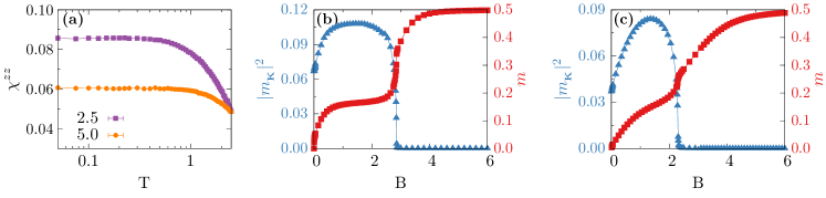
Figure 10: (a) The magnetic susceptibility $\chi^{zz}$ versus the temperature $T$ for the paramagnetic (or the Ising disordered) state. Here we take the parameter ${J_{zz}=1}$, ${h=2.5,5.0}$. The magnetic susceptibility is defined as ${\chi^{zz}={\partial m}/{\partial B}}$ where ${m=(\sum_{i}S_{i}^{z})/N}$ is the dipolar magnetization per site. (b) and (c): Magnetization $m$ (in red) and the magnetic Bragg peak $|m_{{}_{K}}|^{2}$ (in blue) for the three-sublattice state at low temperatures. The parameter we take is ${J_{zz}=1}$ and for (b): ${h=0.25}$, for (c): ${h=0.65}$. All results are calculated through QMC with the system size $L=12$ and ${\beta=80}$. The error bars are much smaller than the points.

Meanwhile, for the three-sublattice ordered state, one can roughly identify two branches of excitations in Fig. 9(b) and clearly identify two branches of excitations in Fig. 9(a). The experimental situation Shen et al. (2019) in TmMgGaO₄ is more close to Fig. 9(b) that shows a reasonable agreement with the experimental data. In Fig. 9(b), we choose the specific parameter ${h/h_{c}^{\text{MF}}\simeq 0.87}$ where $h_{c}^{\text{MF}}$ is the critical field of the mean-field theory. The counting of the branch number immediately brings up a question that the number of branches in the experiment is inconsistent with the number of magnetic sublattices. This question was not raised in Ref. Shen et al., 2019 and is addressed here. In fact, our honest linear spin-wave calculation of the full spectra in the Appendix. A gives three branches of dispersions that correspond to the three-sublattice magnetic structure. The reason that the $S^{z}$-$S^{z}$ correlation looks like two branches is because the selective measurement makes the intensity of part of the excitation spectra rather weak such that the spectra look like two branches. This indicates the incompleteness of the selective measurements. Other dynamic measurements such as optics and THz may avoid the selective measurement issue and provide complementary information about the excitations here.

For the specific TmMgGaO₄ material, the previous neutron scattering experiment shows a tiny spin gap at the $K$ point Shen et al. (2019). This is expected as the model and the system do not have any continuous symmetry to support any gapless Goldstone mode. The reason that the gap is tiny is a common consequence of the quantum order by disorder Savary et al. (2012) for the TFIM with the antiferromagnetic Ising interaction on the triangular lattice. This tiny-gapped mode is sometimes referred as pseudo-Goldstone mode as it appears as a breaking of continuous symmetry at the quadratic or linear spin-wave theory level Savary et al. (2012).

VII More effects from external magnetic field

The external magnetic field not only enriches the phase diagram but also generates more experimental consequences to be examined. In this section, we will first focus on the static properties of the system such as the magnetization and static spin structure factor under the external magnetic field, and then explore the dynamic properties of the system.

VII.1 Susceptibility, magnetization, and non-monotonic ordering

Except in a small parameter regime near the critical point (see Fig. 3) where the magnetic field could drive a re-entrant transition by crossing the three-sublattice ordered one, we do not expect phase transitions upon increasing temperatures with or without the external field for the paramagnetic (or the Ising disordered) state that preserves all the lattice symmetries. This behavior is fundamentally different from those of the three-sublattice ordered state, which can be used to identify these two phases without performing the neutron scattering experiments. The magnetic susceptibility $\chi^{zz}$ as a function of the temperature is calculated via QMC and is plotted in Fig. 10(a). At high temperatures the magnetic susceptibility satisfies the Curie-Weiss law with $\chi^{zz}\simeq{C}/{(T-\Theta_{\text{CW}})}$, where $C$ is the Curie constant and ${\Theta_{\text{CW}}=-{3}J_{zz}/2}$ where one can extract the exchange parameter $J_{zz}$. There is a crossover to the low temperature behavior where $\chi^{zz}$ saturates to a constant. This is because the Hamiltonian does not have any continuous symmetry and the total magnetization is not a good quantum number to label the many-body states. Within a simple mean-field theory, we find the low-temperature $\chi^{zz}$ is given as

$${\chi^{zz}|}_{T\rightarrow 0}\approx\frac{1}{6J_{zz}+2h}.$$ (27)

Compared to the QMC data, we find that at large $h$, they coincide very well. Therefore, one can extract the model parameter $J_{zz}$ and $h$ simply from the high-temperature and low-temperature behaviors of $\chi^{zz}$ if the system is located in the paramagnetic phase. The above relation is especially useful if the ground state of the system is in the Ising disordered phase.

We continue to discuss the magnetization process of the three-sublattice state that can be relevant for the specific material TmMgGaO₄. In the absence of the external magnetic field, the three-sublattice ordering arises from the quantum order-by-disorder mechanism. The spin excitation gap is relatively small (see Fig. 9(a),(b)). This property makes the three-sublattice state fragile against the external magnetic field. A small external field at $B_{c1}$ will cause the closing of the spin gap and drive the system towards the intermediate quasi-plateau state. Here “quasi-plateau” is used as the total magnetization is not conserved. With the increasing external magnetic field, the spin gap re-opens and the intermediate state becomes stable. Further increasing magnetic field the spin gap drops until the system is driven to a polarized state by the magnetic field at $B_{c2}$ above which the system is smoothly connected to the fully polarized one.

The presence of the intermediate quasi-plateau state renders the the magnetization process non-trivial, as it is shown in Fig. 10 from the QMC calculation. For a small $h$, the magnetization curve shows a clear $1/3$ quasi-plateau feature in the intermediate regime. Meanwhile, deep in the quasi-plateau state, the system has an approximate “2-up-1-down” structure that contributes to a robust three-sublattice ordering compared to the case without the external field. Therefore, in the elastic neutron experiments the intensity of the magnetic Bragg peak $|m_{{}_{K}}|^{2}$ (proportional to $|\psi|^{2}$) is expected to show non-monotonic behaviors: deep in the quasi-plateau state the intensity is large, while approaching the three-sublattice state I the intensity is expected to decrease; the intensity is also expected to decrease when the field is large enough where the system becomes nearly polarized (see Fig. 10(b)).

For the case relevant with TmMgGaO₄ where the transverse field $h$ is comparable to the exchange $J_{zz}$, in the quasi-plateau regime the “2-up-1-down” structure is heavily distorted, therefore the quasi-plateau feature of the intermediate regime is not clearly observed in the magnetization curve. Instead, the line shape curves slightly downwards at $B_{c2}$ (see Fig. 10(c)). This feature is found in the magnetization data of TmMgGaO₄ at about 2.5T, which marks the transition field $B_{c2}$ Cevallos et al. (2018); Li et al. (2018); Shen et al. (2019); Li et al. (2020). Above $B_{c2}$ the system becomes polarized, but not fully aligned along the $z$ direction due to the presence of the intrinsic transverse field. In order to allow the magnetization approach the saturation value, a larger external field has to be applied. This feature is in a stark contrast to ordinary systems where the internal transverse field is absent. For the magnetic Bragg peak $|m{{}_{K}}|^{2}$, the non-monotonic behavior persists with large transverse fields (see Fig. 10(c)).

VII.2 Dynamic properties in magnetic fields

Here we discuss the dynamical properties in presence of external magnetic field. With applying small external magnetic field, the gap first decreases and closes at $B_{c1}$. As $B_{c1}$ is typically small, this phenomenon is subtle and can be hard to be observed experimentally. With increasing magnetic field the system gap reopens across $B_{c1}$ as it enters the intermediate “II” regime. In the “II” regime the gap behaves non-monotonically: the gap first increases, reaches maximum and drops, until the system becomes polarized at $B_{c2}$ via a first-order transition. As this transition being first-order, the gap does not close across $B_{c2}$.

We have calculated the spin excitation spectra with magnetic field, as is shown in Fig. 9(d)-(f). From Fig. 9(d) we can clearly see three spin-wave branches, consistent with the three-sublattice magnetic order. Therefore, the “selection rule” breaks down with magnetic field. Another observation is that there remains non-zero intensity even in the fully polarized state, see Fig. 9(f). This is a peculiar feature for our non-degenerate dipole-multipole doublet systems due to the intrinsic transverse field: the spins are tilted to acquire non-zero transverse components, which results the non-vanishing intensity in the polarized state.

VIII Discussion

VIII.1 Summary for TmMgGaO₄

In this paper, we have performed a theoretical study on the triangular lattice transverse field Ising model relevant with the TmMgGaO₄ material. We clarify the intrinsic origin of transverse field of this material as the crystal field splitting. We established the full phase diagram by combining the mean-field theory and the QMC simulation. We discuss the continuous symmetry and BKT physics that emerge in the thermal melting and at the quantum critical point. We explain the properties of phases in the neutron scattering measurement and the thermodynamic experiments. The available experimental data show that this material at zero field is well consistent with the TRIM with the three-sublattice intertwined dipolar and multipolar ordered ground state.

We mention a couple recent works on TmMgGaO₄ and the transverse field Ising model on triangular lattice. A recent numerical-oriented work Li et al. (2020) explored our proposed effective model for TmMgGaO₄ using more updated numerical techniques and focused on the numerical aspects of the model. Their results supported the validity of the TFIM for TmMgGaO₄. Ref. Li et al., 2020 suggested the system first enters the BKT phase at $\sim 4$K and then enters the 3-sublattice ordered state at $\sim 1$K. This differs from the results of the current work, where we have $\sim 1$K for the upper BKT transition and $\sim 0.5$K for the lower one. They further established the roton mode at the $M$ point inside the three-sublattice ordered state. This is probably due to the presence of the second-neighbor interaction. One may understand this in analogous with the supersolidity and the roton mode in the spin-1/2 XXZ model or repulsive hard-core boson model at half-filling on the triangular lattice where the roton condensation leads to the $S^{z}$ order Wessel and Troyer (2005); Melko et al. (2005) on top of the transverse component order. The difference is that, the TFIM here develops an emergent U(1) symmetry and cannot have supersolidity while the XXZ model has a global U(1) symmetry. One may further consider the effect of the dipole-dipole interaction and other effects on this roton mode.

Another quite recent experimental work Li et al. (2020) supplemented the early thermodynamic results Li et al. (2018) with neutron diffraction measurements and corrected the early claim of a pure Ising model with more analysis. In the new work Li et al. (2020) the authors added the transverse field and suggested the Mg/Ga site disorder could create a (random) distribution of the transverse field. They argued that this site disorder could be the origin of their proposed “partial up-up-down” order. Based on the neutron diffraction and thermodynamic measurements, Ref. Li et al., 2018 compared the parameters of different couplings of the model with finite-size exact diagonalization calculation and supported the proposal of a TFIM with random disorders. Since Ref. Li et al., 2018 raised the possible issue of random disorders, we agree that the quantitative behaviors of the thermodynamic results might be more sensitive to disorder effects on the exchange and “$g$” factors as well as the residual coupling to the high-order multipolar moments. On the other hand, the random exchange and/or the random transverse field would lead to the line-broadening with a similar range of energies in the spin-wave spectrum Li et al. (2018). Although a well-defined spin-wave spectrum with a clear dispersion was recorded in the inelastic neutron scattering measurement and reported in Ref. Shen et al., 2019, we still think more data-rich experiments are needed at this stage if one hopes to extract more quantitive information. For example, one could carry out the inelastic neutron scattering measurements as a function of the external magnetic field and establish the excitation spectrum in the (more robust) three-sublattice ordered state of the phase II. One can combine the results of zero field and finite fields and give an estimate of the transverse field distribution from the linewidth of the excitations after subtracting the broadening due to the magnon interactions and the instrument resolution.

In our analysis here, we did not consider the random disorder effect that was actually raised after the first online version of the current work in Ref. Li et al., 2018, and were unable to provide or address much more detailed numerical and quantitative aspects that relate to the experiments quantitatively. We focus more on the generic and qualitative physics that may be more robust in the experiments. Regardless of the specific material, it will be interesting to understand the fate of the finite-temperature BKT phase in the presence of quenched random disorders, and this may be analyzed with the perturbative renormalization calculation within the BKT phase.

VIII.2 Connection to upper branch magnetism

In fact, the magnetism of TmMgGaO₄ belongs to the category of systems with “upper branch magnetism”. The notion of “upper branch magnetism” was introduced in Ref. Liu et al., 2019. It refers to the case where the local crystal field environment simply favors a non-magnetic state while the superexchange interaction prefers magnetic states of some sort. For the specific illustrative example in Ref. Liu et al., 2019, the local crystal field ground state is a singlet and the first excited states are a two-fold degenerate doublet. The specific system over there was modelled as an effective spin-1 magnet, and the crystal field splitting was modelled as a single-ion anisotropy for the spin-1 moment.

In what sense is TmMgGaO₄ regarded as “upper branch magnetism”? The magnetism cannot occur if there is no exchange interaction between the Tm local moments. Crudely speaking, it is the exchange interaction that “drag down” the excited energy level. More precisely, it is the non-trivial quantum mechanical interplay between the intrinsic transverse field and the Ising exchange that gives rise to the magnetism and the associated coherent excitation. What do we expect experimentally if the system is controlled more by the single-ion physics? The magnetism will be gone. Despite that, the coherent magnetic excitation would persist. This may occur in some other systems.

VIII.3 Extension to other Tm-based compounds

A series of rare-earth triangular lattice magnets has been summarized in Ref. Liu et al., 2018. We expect that other materials, especially some Tm-based compounds, can be also described by the TFIM, and share similar physics with TmMgGaO₄. The Tm-based magnetism is not a common subject in quantum magnetism of the rare-earth systems. Some of the insights that we learn from TmMgGaO₄ could be applied to other Tm-magnets. In the following, we survey the existing Tm-magnets and explain the physics in them.

VIII.3.1 Tm spinels and Tm pyrochlores

The Tm spinel, MgTm₂Se₄, has been studied by the neutron scattering measurement Reig-i Plessis et al. (2019). The crystal electric field states were carefully studied in Ref. Reig-i Plessis et al., 2019. It turns out that the crystal field ground state and the first excited state are similar to the ones in TmMgGaO₄. They are separated from other excited levels by an energy gap more than 10meV. The wavefunctions of the lowest two states are

$$|\Psi_{g}\rangle = 0.66960|6\rangle+0.14821|3\rangle+0.24361|0\rangle$$ (28)

$$\quad-0.14821|{-3}\rangle+0.66960|{-6}\rangle,$$

$$|\Psi_{e}\rangle = -0.70097|6\rangle-0.092966|3\rangle$$ (29)

$$\quad-0.092966|{-3}\rangle+0.70097|{-6}\rangle,$$

and the energy separation between them is about 0.885meV. Similar to TmMgGaO₄, one could introduce an effective spin-1/2 degree of freedom that operates on these two states. Here, we propose a relevant model for MgTm₂Se₄ would be a transverse field Ising model on the pyrochlore lattice,

$$H_{\text{MgTm${}_{2}$Se${}_{4}$}}=J_{z}\sum_{\langle ij\rangle}S_{i}^{z}S_{j}^{z}-h\sum_{i}S_{i}^{y}-B\sum_{i}(\hat{n}\cdot\hat{z}_{i})S_{i}^{z},$$ (30)

where $\hat{z}_{i}$ is the local $[111]$ axis, $h$ ($B$) is the intrinsic transverse (external magnetic) field, and $\hat{n}$ is the direction of the external magnetic field. Ref. Reig-i Plessis et al., 2019 has suggested a vanishing $g$-factor for the Tm³⁺ ion. Based on our experience and the magnetization measurement in Ref. Reig-i Plessis et al., 2019, however, we think that the field would primarily couple to the local $z$ component of the local moment. The magnetic moment of MgTm₂Se₄ can be read from the saturated magnetization after considering the fact that the magnetic moment is oriented along the local [111] direction of each sublattice. The sign of $J_{z}$ plays an important role in determining the quantum ground state of MgTm₂Se₄. It is ready to obtain that, the Curie-Weiss temperature has ${\Theta_{CW}=J_{z}/2}$ and does not depend on the direction of the probing field. Unfortunately, the Curie-Weiss temperature is unknown for this material. If ${J_{z}>0}$, one could establish a pyrochlore ice U(1) spin liquid ground state when $h$ is small and develop a quantum transition into a disordered state when $h$ is large. If ${J_{z}<0}$, then one simply has the usual phase diagram of the ferromagnetic Ising model.

The Tm-based pyrochlore has rarely been studied. The crystal field levels of Tm₂Ti₂O₇ were computed in Ref. Bertin et al., 2012. It was found that, the crystal field ground state is a singlet with the wavefunction,

$$|\Psi_{g}\rangle=0.147|{6}\rangle-0.692|{3}\rangle-0.692|{-3}\rangle-0.147|{-6}\rangle,$$ (31)

and the first excited state is a doublet with two-fold degeneracy. This crystal field level setting is identical to the specific case that was considered in Ref. Liu et al., 2019. The energy separation between the ground state singlet and the first excited doublet is of the order of 10meV, so it is not in the weak crystal field regime for the rare-earth magnets. It is likely that other isostructural Tm-based pyrochlores could have a smaller crystal field gap and allow more interesting magnetism to happen.

VIII.3.2 Tm honeycomb lattice and Tm Kagomé lattice magnets

Here we extend some of our thoughts to other two-dimensional systems. We start with the honeycomb magnet RNi₃Al₉ where R is the rare-earth ion and Tm is a member of them Yamashita et al. (2011). These materials have both conduction electrons and local moments, so it is a conductor and there is a Kondo physics in some of them. The local moment magnetism is from the rare-earth moments. We focus the discussion on the Tm-based materials. Other materials in this family such as the Yb-based ones could involve Kitaev and other anisotropic spin interactions between the local moments and also worth a further investigation. The magnetization measurement in the single crystal sample of TmNi₃Al₉ is quite similar to the one in TmMgGaO₄, where the out-of-plane response is dominant and the in-plane response is negligible. There are two possibilities for the Tm magnetism in TmNi₃Al₉. The first possibility is that the Tm local moment is a (degenerate) non-Kramers doublet. The other possibility is that the Tm local moment is a non-degenerate dipole-multipole doublet like the one in TmMgGaO₄, and the effective model for the Tm magnetism would be a transverse field Ising model. Due to the presence of the itinerant electrons, the Ising interaction may involve further neighbors. This material develops a magnetic order at $2.9$K from the thermodynamic and transport measurements. From the experience about TmMgGaO₄, we expect a coherent excitation spectrum. This may be confirmed by further experiments with neutron scattering measurements.

The Tm-based Kagomé magnets have been explored recently Ding et al. (2018); Dun et al. (2017, 2016), and effective spin-1/2 degrees of freedom are used to describe the Tm magnetism. Unlike the triangular lattice and the honeycomb lattice, the point group symmetry does not involve an on-site three-fold rotation, and there is no non-Kramers doublet on the Kagomé lattice. Thus there is always an intrinsic splitting between the two relevant crystal field levels of the Tm³⁺ ion. Because the Tm³⁺ singlets are not the same kind of singlets as the ones in TmMgGaO₄, the exchange part of the interaction is not simply be the Ising model.

VIII.3.3 Tm double perovskites

Another class of the Tm magnets is the Tm-based double perovskite. Unlike the rare-earth pyrochlores and the rare-earth triangular lattice magnets, these materials have not been well studied before. Here Tm ions form a FCC lattice. Only two Tm-based double perovskites Ba₂TmSbO₆ and Ba₂TmBiO₆ have been studied Otsuka and Hinatsu (2015). Besides the basic thermodynamic and structural measurements at high temperatures, very little information is known for these two materials. Thus, we cannot extract much more physical understanding for the time being. But these two materials remain as good candidates for frustrated FCC systems with spin-orbit-entangled local moments Li et al. (2017).

VIII.4 General expectation for intrinsic quantum Ising magnets

From our study of TmMgGaO₄ and the discussion on many other Tm-based magnets, we think the intrinsic quantum Ising magnets can widely exist in nature. The Tm³⁺ ion in the D_3d crystal field is a bit special due to the high symmetry group of the D_3d point group and the symmetry demanded crystal field singlets. In more general cases Chen (2019), we do not have such a high symmetry point group, and thus we think the intrinsic transverse field can be more common in rare-earth magnets with lower crystal field symmetries. To further remove the degeneracy, we have to get rid of the Kramers’ theorem. It is then interesting to search for the intrinsic quantum Ising magnets among the rare-earth magnets with low crystal field symmetries and integer-spin local moments.

Appendix A Results from linear spin-wave theory

In this appendix, we provide the linear spin-wave theory and results for the magnetic excitations in the three-sublattice magnetic orders. The reason that we do this calculation is to clarify the discrepancy between the number of the magnetic sublattices and the numbers of the measured magnon branches.

For the three-sublattice magnetic ordered states, the system has $\sqrt{3}\times\sqrt{3}$ magnetic unit cell, each spin can be labeled by combination of magnetic unit cell position ${\mathbf{r}}$ and sublattice index $s$ ($s=1,2,3$). The mean-field ground-states can be obtained by Weiss mean-field theory, where the mean-field spin orientations for each sublattices $s$ can be labeled by unit vector $\mathbf{n}_{s}$. Then one can always associate two unit vectors ${\mathbf{u}_{s}\cdot\mathbf{n}_{s}=0}$ and ${\mathbf{v}_{s}=\mathbf{n}_{s}\times\mathbf{u}_{s}}$ so that $\mathbf{n}_{s}$, $\mathbf{u}_{s}$ and $\mathbf{v}_{s}$ are orthogonal with each other. Next we perform Holstein-Primakoff transformation for the spin operator $\mathbf{S}_{{\mathbf{r}}s}$,

$$\mathbf{n}_{s}\cdot\mathbf{S}_{{\mathbf{r}}s} = S-b_{{\mathbf{r}}s}^{\dagger}b_{{\mathbf{r}}s},$$ (32)

$$(\mathbf{u}_{s}+i\mathbf{v}_{s})\cdot\mathbf{S}_{{\mathbf{r}}s} = ({2S-b_{{\mathbf{r}}s}^{\dagger}b_{{\mathbf{r}}s}})^{\frac{1}{2}}b_{{\mathbf{r}}s},$$ (33)

$$(\mathbf{u}_{s}-i\mathbf{v}_{s})\cdot\mathbf{S}_{{\mathbf{r}}s} = b_{{\mathbf{r}}s}^{\dagger}({2S-b_{{\mathbf{r}}s}^{\dagger}b_{{\mathbf{r}}s}})^{\frac{1}{2}}.$$ (34)

After performing Fourier transformation

$$b_{{\mathbf{r}}s}=\sqrt{\frac{3}{N}}\sum_{\mathbf{k}\in{\overline{\text{BZ}}}}b_{\mathbf{k}s}e^{i\mathbf{R}_{{\mathbf{r}}s}\cdot\mathbf{k}},$$ (35)

the spin Hamiltonian can be rewritten in terms of boson bilinears as

$$H_{\text{sw}}=\frac{1}{2}\sum_{\mathbf{k}\in{\overline{\text{BZ}}}}\Psi(\mathbf{k}){}^{\dagger}h(\mathbf{k})\Psi(\mathbf{k})+cosnt.,$$ (36)

where

$$\Psi(\mathbf{k})=[b_{\mathbf{k}1},b_{\mathbf{k}2},b_{\mathbf{k}3},b_{\mathbf{-k}1}^{\dagger},b_{\mathbf{-k}2}^{\dagger},b_{\mathbf{-k}3}^{\dagger}]^{T}$$ (37)

and $h(\mathbf{k})$ is a ${6\times 6}$ Hermitian matrix, and $\overline{\text{BZ}}$ is the magnetic Brillouin zone. Then we can Bogoliubov diagonalize $H_{\text{sw}}$ with ${\Psi(\mathbf{k})=T_{\mathbf{k}}\Phi(\mathbf{k})}$, where

$$\Phi(\mathbf{k})=[\beta_{\mathbf{k}1},\beta_{\mathbf{k}2},\beta_{\mathbf{k}3},\beta_{\mathbf{-k}1}^{\dagger},\beta_{\mathbf{-k}2}^{\dagger},\beta_{-\mathbf{k}3}^{\dagger}]^{T},$$ (38)

is the diagonalized basis and $T_{\mathbf{k}}$ is the transformation matrix. Details of diagonalization can be referred to Petit, S. (2011); Wallace (1962); Toth and Lake (2015). The diagonalized Hamiltonian reads

$$H_{\text{sw}} = \frac{1}{2}\sum_{\mathbf{k}\in\overline{\text{BZ}}}\Phi(\mathbf{k}){}^{\dagger}E(\mathbf{k})\Phi(\mathbf{k})+const.$$ (39)

$$= \sum_{\mathbf{k}\in\overline{\text{BZ}}}\omega_{\mathbf{k}s}\beta_{\mathbf{k}s}^{\dagger}\beta_{\mathbf{k}s}+const.,$$

where $E(\mathbf{k})=\mbox{diag}[\omega_{\mathbf{k}1},\omega_{\mathbf{k}2},\omega_{\mathbf{k}3},\omega_{-\mathbf{k}1},\omega_{-\mathbf{k}2},\omega_{-\mathbf{k}3}]$. Within this formalism, we find that the coherent contribution to the ${\mathcal{S}}^{zz}$ correlator takes the following form

$${\mathcal{S}}^{zz}(\mathbf{k},\omega)$$

$$\quad=\frac{S}{6}\sum_{s=1}^{3}[T_{\mathbf{k}}^{\dagger}\mathbf{U}^{z}(\mathbf{U^{z})}^{\dagger}T_{\mathbf{k}}]_{s+3,s+3}\delta(\omega-\omega_{-\mathbf{k}s}),$$ (40)

where $\mathbf{U}^{z}$ is a $6$-dimensional vector

$$\mathbf{U}^{z} = [u_{1}^{z}+iv_{1}^{z},u_{2}^{z}+iv_{2}^{z},u_{3}^{z}+iv_{3}^{z},$$ (41)

$$\,\,u_{1}^{z}-iv_{1}^{z},u_{2}^{z}-iv_{2}^{z},u_{3}^{z}-iv_{3}^{z}]^{T}.$$

Due to the quantum fluctuation, the magnetic orders are suppressed from the mean-field values, as a result, the bandwidth of the single-magnon spectra will be renormalized. This is a well-known feature of the linear spin-wave theory Chernyshev and Zhitomirsky (2009). If one is interested in more quantitative features, one could use more involved renormalized spin-wave theory that takes into account the suppression of the magnetic orders by quantum fluctuations Chernyshev and Zhitomirsky (2009). However, the linear spin-wave theory does provide a useful understanding of the structure of the magnetic excitations. In our spin-wave calculation, there are three branches of dispersions that are consistent with the number of the magnetic sublattices.

References

- Wannier (1950) G. Wannier, Phys. Rev. 79, 357 (1950).
- Kanô and Naya (1953) K. Kanô and S. Naya, Prog. Theor. Exp. Phys. 10, 158 (1953).
- Harris et al. (1997) M. J. Harris, S. Bramwell, D. McMorrow, T. Zeiske, and K. Godfrey, Phys. Rev. Lett. 79, 2554 (1997).
- Ramirez et al. (1999) A. P. Ramirez, A. Hayashi, R. J. Cava, R. Siddharthan, and B. Shastry, Nature 399, 333 (1999).
- Moessner et al. (2000) R. Moessner, S. L. Sondhi, and P. Chandra, Phys. Rev. Lett. 84, 4457 (2000).
- Moessner and Sondhi (2001) R. Moessner and S. L. Sondhi, Phys. Rev. B 63, 224401 (2001).
- Hermele et al. (2004) M. Hermele, M. P. Fisher, and L. Balents, Phys. Rev. B 69, 064404 (2004).
- Röchner et al. (2016a) J. Röchner, L. Balents, and K. P. Schmidt, Phys. Rev. B 94, 201111 (2016a).
- Nikolić and Senthil (2005) P. Nikolić and T. Senthil, Phys. Rev. B 71, 024401 (2005).
- Villain et al. (1980) J. Villain, R. Bidaux, J.-P. Carton, and R. Conte, J. Phys. France 41, 1263 (1980).
- Shender (1982) E. Shender, Sov. Phys. JETP 56, 178 (1982).
- Powalski et al. (2013) M. Powalski, K. Coester, R. Moessner, and K. P. Schmidt, Phys. Rev. B 87, 054404 (2013).
- Schmidt (2013) K. P. Schmidt, Phys. Rev. B 88, 035118 (2013).
- Coester et al. (2013) K. Coester, W. Malitz, S. Fey, and K. P. Schmidt, Phys. Rev. B 88, 184402 (2013).
- Röchner et al. (2016b) J. Röchner, L. Balents, and K. P. Schmidt, Phys. Rev. B 94, 201111 (2016b).
- Koziol et al. (2019) J. Koziol, S. Fey, S. C. Kapfer, and K. P. Schmidt, Phys. Rev. B 100, 144411 (2019).
- Fey et al. (2019) S. Fey, S. C. Kapfer, and K. P. Schmidt, Phys. Rev. Lett. 122, 017203 (2019).
- Chen (2019) G. Chen, Phys. Rev. Research 1, 033141 (2019).
- Coldea et al. (2010) R. Coldea, D. A. Tennant, E. M. Wheeler, E. Wawrzynska, D. Prabhakaran, M. Telling, K. Habicht, P. Smeibidl, and K. Kiefer, Science 327, 177 (2010).
- Kinross et al. (2014) A. W. Kinross, M. Fu, T. J. Munsie, H. A. Dabkowska, G. M. Luke, S. Sachdev, and T. Imai, Phys. Rev. X 4, 031008 (2014).
- Cabrera et al. (2014) I. Cabrera, J. D. Thompson, R. Coldea, D. Prabhakaran, R. I. Bewley, T. Guidi, J. A. Rodriguez-Rivera, and C. Stock, Phys. Rev. B 90, 014418 (2014).
- Suga (2008) S. Suga, J. Phys. Soc. Jpn. 77, 074717 (2008).
- Wang et al. (2018) Z. Wang, T. Lorenz, D. I. Gorbunov, P. T. Cong, Y. Kohama, S. Niesen, O. Breunig, J. Engelmayer, A. Herman, J. Wu, K. Kindo, J. Wosnitza, S. Zherlitsyn, and A. Loidl, Phys. Rev. Lett. 120, 207205 (2018).
- Wang et al. (2018) Z. Wang, J. Wu, W. Yang, A. K. Bera, D. Kamenskyi, A. T. M. N. Islam, S. Xu, J. M. Law, B. Lake, C. Wu, and A. Loidl, Nature 554, 219 (2018).
- He et al. (2006) Z. He, T. Taniyama, and M. Itoh, Phys. Rev. B 73, 212406 (2006).
- Cui et al. (2019) Y. Cui, H. Zou, N. Xi, Z. He, Y. X. Yang, L. Shu, G. H. Zhang, Z. Hu, T. Chen, R. Yu, J. Wu, and W. Yu, Phys. Rev. Lett. 123, 067203 (2019).
- Shen et al. (2019) Y. Shen, C. Liu, Y. Qin, S. Shen, Y.-D. Li, R. Bewley, A. Schneidewind, G. Chen, and J. Zhao, Nature Communications 10, 4530 (2019).
- Cevallos et al. (2018) F. A. Cevallos, K. Stolze, T. Kong, and R. Cava, Mater. Res. Bull. 105, 154 (2018).
- Li et al. (2018) Y. Li, S. Bachus, Y. Tokiwa, A. A. Tsirlin, and P. Gegenwart, arXiv:1804.00696 (2018).
- Li et al. (2020) Y. Li, S. Bachus, H. Deng, W. Schmidt, H. Thoma, V. Hutanu, Y. Tokiwa, A. A. Tsirlin, and P. Gegenwart, Phys. Rev. X 10, 011007 (2020).
- Liu et al. (2018) C. Liu, Y.-D. Li, and G. Chen, Phys. Rev. B 98, 045119 (2018).
- Bonville et al. (2016) P. Bonville, S. Guitteny, A. Gukasov, I. Mirebeau, S. Petit, C. Decorse, M. C. Hatnean, and G. Balakrishnan, Phys. Rev. B 94, 134428 (2016).
- Chen (2016) G. Chen, Phys. Rev. B 94, 205107 (2016).
- Huang et al. (2014) Y.-P. Huang, G. Chen, and M. Hermele, Phys. Rev. Lett. 112, 167203 (2014).
- Li and Chen (2017) Y.-D. Li and G. Chen, Phys. Rev. B 95, 041106 (2017).
- Li et al. (2016a) Y.-D. Li, X. Wang, and G. Chen, Phys. Rev. B 94, 201114 (2016a).
- Li et al. (2016b) Y.-D. Li, X. Wang, and G. Chen, Phys. Rev. B 94, 035107 (2016b).
- Lhotel et al. (2015) E. Lhotel, S. Petit, S. Guitteny, O. Florea, M. Ciomaga Hatnean, C. Colin, E. Ressouche, M. R. Lees, and G. Balakrishnan, Phys. Rev. Lett. 115, 197202 (2015).
- Anand et al. (2015) V. K. Anand, A. K. Bera, J. Xu, T. Herrmannsdörfer, C. Ritter, and B. Lake, Phys. Rev. B 92, 184418 (2015).
- Bertin et al. (2015) A. Bertin, P. Dalmas de Réotier, B. Fåk, C. Marin, A. Yaouanc, A. Forget, D. Sheptyakov, B. Frick, C. Ritter, A. Amato, C. Baines, and P. J. C. King, Phys. Rev. B 92, 144423 (2015).
- Xu et al. (2015) J. Xu, V. K. Anand, A. K. Bera, M. Frontzek, D. L. Abernathy, N. Casati, K. Siemensmeyer, and B. Lake, Phys. Rev. B 92, 224430 (2015).
- Hatnean et al. (2015) M. C. Hatnean, M. R. Lees, O. A. Petrenko, D. S. Keeble, G. Balakrishnan, M. J. Gutmann, V. V. Klekovkina, and B. Z. Malkin, Phys. Rev. B 91, 174416 (2015).
- Petit et al. (2016) S. Petit, E. Lhotel, B. Canals, M. C. Hatnean, J. Ollivier, H. Mutka, E. Ressouche, A. Wildes, M. Lees, and G. Balakrishnan, Nat. Phys. 12, 746 (2016).
- Benton (2016) O. Benton, Phys. Rev. B 94, 104430 (2016).
- Dalmas de Réotier et al. (2017) P. Dalmas de Réotier, A. Yaouanc, A. Maisuradze, A. Bertin, P. J. Baker, A. D. Hillier, and A. Forget, Phys. Rev. B 95, 134420 (2017).
- Mauws et al. (2018) C. Mauws, A. M. Hallas, G. Sala, A. A. Aczel, P. M. Sarte, J. Gaudet, D. Ziat, J. A. Quilliam, J. A. Lussier, M. Bieringer, H. D. Zhou, A. Wildes, M. B. Stone, D. Abernathy, G. M. Luke, B. D. Gaulin, and C. R. Wiebe, Phys. Rev. B 98, 100401 (2018).
- Pe çanha Antonio et al. (2019) V. Pe çanha Antonio, E. Feng, X. Sun, D. Adroja, H. C. Walker, A. S. Gibbs, F. Orlandi, Y. Su, and T. Brückel, Phys. Rev. B 99, 134415 (2019).
- Sibille et al. (2015) R. Sibille, E. Lhotel, V. Pomjakushin, C. Baines, T. Fennell, and M. Kenzelmann, Phys. Rev. Lett. 115, 097202 (2015).
- Sibille et al. (2019) R. Sibille, N. Gauthier, E. Lhotel, V. Porée, V. Pomjakushin, R. A. Ewings, T. G. Perring, J. Ollivier, A. Wildes, C. Ritter, et al., arXiv:1912.00928 (2019).
- Gaudet et al. (2019) J. Gaudet, E. M. Smith, J. Dudemaine, J. Beare, C. R. C. Buhariwalla, N. P. Butch, M. B. Stone, A. I. Kolesnikov, G. Xu, D. R. Yahne, K. A. Ross, C. A. Marjerrison, J. D. Garrett, G. M. Luke, A. D. Bianchi, and B. D. Gaulin, Phys. Rev. Lett. 122, 187201 (2019).
- Gao et al. (2019) B. Gao, T. Chen, D. W. Tam, C.-L. Huang, K. Sasmal, D. T. Adroja, F. Ye, H. Cao, G. Sala, M. B. Stone, C. Baines, J. A. T. Verezhak, H. Hu, J.-H. Chung, X. Xu, S.-W. Cheong, M. Nallaiyan, S. Spagna, M. Brian Maple, A. H. Nevidomskyy, E. Morosan, G. Chen, and P. Dai, Nature Physics 15, 1052 (2019).
- Yao et al. (2020) X.-P. Yao, Y.-D. Li, and G. Chen, Phys. Rev. Research 2, 013334 (2020).
- Lago et al. (2010) J. Lago, I. Živković, B. Z. Malkin, J. Rodriguez Fernandez, P. Ghigna, P. Dalmas de Réotier, A. Yaouanc, and T. Rojo, Phys. Rev. Lett. 104, 247203 (2010).
- Gao et al. (2018) S. Gao, O. Zaharko, V. Tsurkan, L. Prodan, E. Riordan, J. Lago, B. Fåk, A. R. Wildes, M. M. Koza, C. Ritter, P. Fouquet, L. Keller, E. Canévet, M. Medarde, J. Blomgren, C. Johansson, S. R. Giblin, S. Vrtnik, J. Luzar, A. Loidl, C. Rüegg, and T. Fennell, Phys. Rev. Lett. 120, 137201 (2018).
- (55) C. Liu, H. Wei, and G. Chen, unpublished .
- Note (1) Yao Shen, Private communication.
- Isakov and Moessner (2003) S. Isakov and R. Moessner, Phys. Rev. B 68, 104409 (2003).
- Wang et al. (2017) Y.-C. Wang, Y. Qi, S. Chen, and Z. Y. Meng, Phys. Rev. B 96, 115160 (2017).
- Blankschtein et al. (1984) D. Blankschtein, M. Ma, A. N. Berker, G. S. Grest, and C. Soukoulis, Phys. Rev. B 29, 5250 (1984).
- Chen et al. (2017) J. Chen, H.-J. Liao, H.-D. Xie, X.-J. Han, R.-Z. Huang, S. Cheng, Z.-C. Wei, Z.-Y. Xie, and T. Xiang, Chinese Physics Letters 34, 050503 (2017).
- Ortiz et al. (2012) G. Ortiz, E. Cobanera, and Z. Nussinov, Nuclear Physics B 854, 780 (2012).
- Zhang (2019) L. Zhang, Phys. Rev. Lett. 123, 230601 (2019).
- Biswas and Damle (2018) S. Biswas and K. Damle, Phys. Rev. B 97, 085114 (2018).
- Damle (2015) K. Damle, Phys. Rev. Lett. 115, 127204 (2015).
- Mydosh and Oppeneer (2014) J. A. Mydosh and P. M. Oppeneer, Philosophical Magazine 94, 3642 (2014).
- Smerald and Shannon (2013) A. Smerald and N. Shannon, Phys. Rev. B 88, 184430 (2013).
- Savary et al. (2012) L. Savary, K. A. Ross, B. D. Gaulin, J. P. C. Ruff, and L. Balents, Phys. Rev. Lett. 109, 167201 (2012).
- Li et al. (2020) H. Li, Y.-D. Liao, B.-B. Chen, X.-T. Zen, X.-L. Sheng, Y. Qi, Z. Y. Meng, and W. Li, Nat. Commun. 11, 1111 (2020).
- Wessel and Troyer (2005) S. Wessel and M. Troyer, Phys. Rev. Lett. 95, 127205 (2005).
- Melko et al. (2005) R. G. Melko, A. Paramekanti, A. A. Burkov, A. Vishwanath, D. N. Sheng, and L. Balents, Phys. Rev. Lett. 95, 127207 (2005).
- Liu et al. (2019) C. Liu, F.-Y. Li, and G. Chen, Phys. Rev. B 99, 224407 (2019).
- Reig-i Plessis et al. (2019) D. Reig-i Plessis, A. Cote, S. van Geldern, R. D. Mayrhofer, A. A. Aczel, and G. J. MacDougall, Phys. Rev. Materials 3, 114408 (2019).
- Bertin et al. (2012) A. Bertin, Y. Chapuis, P. D. de Réotier, and A. Yaouanc, J. Phys. Condens. Matter 24, 256003 (2012).
- Yamashita et al. (2011) T. Yamashita, S. Ohara, and I. Sakamoto, Journal of the Physical Society of Japan 80, SA080 (2011).
- Ding et al. (2018) Z.-F. Ding, Y.-X. Yang, J. Zhang, C. Tan, Z.-H. Zhu, G. Chen, and L. Shu, Phys. Rev. B 98, 174404 (2018).
- Dun et al. (2017) Z. L. Dun, J. Trinh, M. Lee, E. S. Choi, K. Li, Y. F. Hu, Y. X. Wang, N. Blanc, A. P. Ramirez, and H. D. Zhou, Phys. Rev. B 95, 104439 (2017).
- Dun et al. (2016) Z. L. Dun, J. Trinh, K. Li, M. Lee, K. W. Chen, R. Baumbach, Y. F. Hu, Y. X. Wang, E. S. Choi, B. S. Shastry, A. P. Ramirez, and H. D. Zhou, Phys. Rev. Lett. 116, 157201 (2016).
- Otsuka and Hinatsu (2015) S. Otsuka and Y. Hinatsu, J. Solid State Chem. 227, 132 (2015).
- Li et al. (2017) F.-Y. Li, Y.-D. Li, Y. Yu, A. Paramekanti, and G. Chen, Phys. Rev. B 95, 085132 (2017).
- Petit, S. (2011) Petit, S., JDN 12, 105 (2011).
- Wallace (1962) D. C. Wallace, Phys. Rev. 128, 1614 (1962).
- Toth and Lake (2015) S. Toth and B. Lake, Journal of Physics: Condensed Matter 27, 166002 (2015).
- Chernyshev and Zhitomirsky (2009) A. L. Chernyshev and M. E. Zhitomirsky, Phys. Rev. B 79, 144416 (2009).