A Tutorial for Joint Modeling of Longitudinal and Time-to-Event Data in R

Abstract

In biostatistics and medical research, longitudinal data are often composed of repeated assessments of a variable (e.g., blood pressure or other biomarkers) and dichotomous indicators to mark an event of interest (e.g., recovery from disease, or death). Consequently, joint modeling of longitudinal and time-to-event data has generated much interest in these disciplines over the previous decade. In psychology, too, often we are interested in relating individual trajectories (e.g., cognitive performance or well-being across many years) and discrete events (e.g., death, diagnosis of dementia, or of depression). Yet, joint modeling are rarely applied in psychology and social sciences more generally. This tutorial presents an overview and general framework for joint modeling of longitudinal and time-to-event data, and fully illustrates its application in the context of a behavioral (cognitive aging) study. We discuss practical topics, such as model selection and comparison for both longitudinal and time-to-event data, choice of joint modeling parameterization, and interpretation of model parameters. To do so, we examined seven frequently used packages for joint modeling in the R language and environment. We concluded that of these, JMbayes is especially attractive due to its flexibility, its various parameterizations of the association structure, and for its powerful and fully Bayesian implementation. We make available the R syntax to apply the JMbayes package within our example.

1 Introduction

In many research settings, it is very common to record longitudinal observations that correspond to responses on continuous measures alongside dichotomous indicators to mark the occurrence of an event of interest. A prototypical example in clinical research is the repeated assessment of biological measures (e.g., blood pressure, antibody affinity, cholesterol level) that may relate to an event such as death, recovery from a disease, or disease diagnosis. In psychological research, much interest evolves around the association between long-term individual trajectories of cognitive performance and imminent death (e.g., terminal decline or terminal drop hypotheses; kleemeier1962; riegel1972).

Methods for the separate analysis of such outcomes are well established in the literature, and these frequently include the use of mixed-effects models for the longitudinal portion of the data and the Cox proportional hazards model for the time-to-event data (Laird_1982; cox1972). However, the repeated measurements of the same individual are most likely related to the event, making them endogenous. This means that the measurement value at a given time point is informative about the future occurrence (or non-occurrence) of the event of interest. Likewise, the longitudinal trajectory is related to, and shaped by, the occurrence of the event. Separate analyses of such data cannot account for this endogeneity and cannot inform about the associative strength between the two. A tentative solution to this problem is a two-step approach, whereby estimated parameters from the mixed-effects models are used as covariates in the time-to-event model. Yet, this approach has been shown to suffer from increased bias in estimation and loss of efficiency (prentice1982covariate; rizopoulos_book). Joint models simultaneously estimate both longitudinal and time-to-event components and are better suited for analyzing such data because they estimate jointly the relative risk of the time-to-event outcome contingent upon the longitudinal outcome (Wulfsohn1997; Song_2002; Henderson2000; hogan1997mixture; tsiatis2004joint; gould_joint_2015; Papageorgiou_2019).

Joint modeling is increasingly used in medical research (see for example Rizopoulos_EuroIntervention; nunez2014red; thabut2013survival; abdi2013impact; mauritz2011usefulness; sene_shared_2014; brown2003bayesian; he2016joint). However, joint models remain conspicuously absent in psychological and behavioral research, despite the proliferation of data that could be analyzed more effectively using this powerful methodology, rather than by using a two-step estimation procedure. For example, given world-wide increases in human life expectancy (and corresponding increases in populations of elders), it will become increasingly important to understand how long-term changes in cognitive, personality, emotional, and other individual behavioral characteristics are related both to specific health-related outcomes (depression, stroke, dementia) and to longevity, or risk of death (world2015world). We found only a few behavioral studies using joint models to evaluate such associations (Ghisletta_2006; ghisletta2008application; McArdle_2005; muniz2011; Muniz_2018) and we believe that the lack of an accessible and clear guidance for implementing such models remains an obstacle preventing non-expert users from applying them skillfully, or from adopting them at all.

This tutorial is therefore aimed at elucidating features of the joint modeling framework for longitudinal and time-to-event data for users familiar with mixed-effects and time-to-event (a.k.a. survival) models. We initially reviewed the seven currently available joint-modeling packages in the open-source R environment for statistical computing (R). The seven packages are JM, JMbayes, joineR, lcmm, frailtypack, rstanarm and bamlss, which are described in tables 9, 10, 11 , 12, 13, 14 and 15, respectively. We concluded that, at present, the JMbayes package (JMbayes) is the most comprehensive and extensible, and thus chose it as the basis for this tutorial. Note that a range of tools allowing one to perform joint modeling are available for other standard statistical software such as SAS/STAT, Stata, WinBUGS, and JAGS (see Papageorgiou_2019, and references therein for more details).

JMbayes provides a framework wherein one or more characteristics from the longitudinal submodel can be flexibly parameterized as linear predictors in the time-to-event submodel. This flexibility is important because the relation between the continuous variable and the event of interest may take several functional forms, each of which may imply a different theoretical interpretation. For example, the longitudinal process can be specified in relatively simple terms (e.g., individual random effects about the intercept and the linear slope within a mixed-effects submodel), or in more complex non-linear spline effects, each of which can be linked to the time-to-event process with any of several association structures. JMbayes also allows for inclusion of multivariate longitudinal processes and for stratification criteria in the time-to-event submodel. Also, estimation of joint models, which are inherently complex, can be computationally intensive. Per its name, the JMbayes package relies on a Bayesian analytical approach, which is very attractive for applications where classical maximum likelihood estimation often encounters nonidentifiability issues yielding unreliable inferential conclusions. Indeed, Bayesian analysis using Markov chain Monte Carlo (MCMC) estimation can yield very precise point estimates without reliance on asymptotic assumptions (robert2004monte). JMbayes also provides useful diagnostic measures for evaluating MCMC convergence and for evaluating relative model fit.

We note that the aim of this tutorial is not to replace the JMbayes documentation, which provides in-depth methodological detail and supplementary R code (JMbayes; rizopoulos2017package). Here, our goal is to complement this information with a more user-oriented, applied perspective, so that non-expert users may successfully carry out analyses using joint models. For the sake of brevity and clarity, we do not provide an exhaustive treatment of all features of joint modeling from the applications, but we nevertheless briefly discuss some of them at the end of the tutorial. We begin by describing the statistical framework for joint modeling. We then discuss required software packages, describe the data set used for this tutorial, and finally present example analyses to illustrate the use of joint modeling for behavioral data analysis. We provide the data and the full syntax of our application as Supplementary material.

2 Statistical Framework

The joint model, first described by Wulfsohn1997, consists of two submodels: a mixed-effects submodel for the longitudinal data and a time-to-event submodel for the time-to-event data. The two submodels are joined by allowing the time-to-event submodel to depend on some characteristics of the longitudinal submodel potentially in various ways. The defining feature of the joint model is that longitudinal and time-to-event data are modeled simultaneously with respect to a conditional joint density, rather than separately with two marginal and independent densities (see e.g., Rizopoulos_JASA, for further technical details). Consequently, the effects of the longitudinal submodel on the time-to-event submodel are explicitly specified, and, at the same time, the parameter estimates of the former are also conditioned on the latter submodel (i.e., the longitudinal submodel is more accurately estimated by including the time-to-event data than without them, if endogeneity occurs). We discuss first the longitudinal submodel, then the time-to-event submodel, and finally several parametrization options to associate the two within the joint model.

2.1 The Mixed-Effects Submodel

Longitudinal data here consist of repeated measurements of the same outcome for each study participant over a given period of time. Repeated measurements for the same individual are typically correlated, and therefore each individual in the population is expected to have his or her own subject-specific response pattern over time. The mixed-effects model (Laird_1982) accounts for this between person variability by estimating person specific random effects around the parameters that are invariant across individuals (fixed effects).

Let $y_{i}(t)$ denote the measurement on $y$ for individual $i$ ($i=1,\dots,N$) at time $t$ ($t=1,\dots,T^{*}_{i}$), where $T^{*}_{i}$ is the time-to-event for individual $i$. The model assumes that $y_{i}(t)$ is the observed measured value, which deviates from the true unobserved value $\mu_{i}(t)$ by the amount of error $\epsilon_{i}(t)$, where $\epsilon_{i}(t)\sim\mathcal{N}(0,\sigma^{2})$, normally distributed around 0 with variance $\sigma^{2}$. The longitudinal submodel can then be written as

$$\mu_{i}(t) =X_{i}(t)\beta+Z_{i}(t)b_{i},\quad\text{or}$$ (1)

$$=f(X_{i}(t))+f_{i}(Z_{i}(t)),$$

where $b_{i}$ denotes the vector of random effects for individual $i$ with $b_{i}\sim\mathcal{N}(0,D)$, and $D$ is the variance-covariance matrix of the random effects (typically a $2\times 2$ unstructured matrix with random intercept and random slope effects). $X_{i}(t)$ and $Z_{i}(t)$ represent the design matrix containing the predictors for the fixed-effects regression coefficients $\beta$ and for the random-effects regression coefficients $b_{i}$, respectively (typically $b_{0i}$ and $b_{1i}$ for random intercept and slope effects).

The second line of Equation (1) represents the notation when $\mu_{i}(t)$ is modeled non-parametrically via a spline approach (illustrated below). $f(\cdot)$ and $f_{i}(\cdot)$ represent the spline function for the fixed and, respectively, random components.

2.2 The Time-to-Event Submodel

Time-to-event, or survival, analysis refers to statistical methods for analyzing time-to-event data. An event time is the time elapsed up to the occurrence of an event of interest (such as death or disease diagnostic), given that it has not previously occurred yet. Time-to-event data are characterized by the fact that the event of interest may not have occurred for every participant during the duration of the study. This particular type of missing data is analogously treated as data of a participant who drops out before the end of the study, and both scenarios constitute right censorship. Time-to-event analysis is particularly appropriate to analyze right-censored data.

There are different models for time-to-event data (kaplan1958nonparametric). Probably, the most popular is the semi-parametric Cox proportional hazard (PH) model (cox1972), which is a regression model wherein covariates are assumed to have a multiplicative effect on the hazard for an event. The Cox PH model has the particularity of estimating the baseline hazard function non-parametrically. If there is a theoretical reason to suppose that the baseline hazard function has a particular parametric form (typically Weibull, Gamma or Exponential), a parametric model can be specified. Most often, however, an analyst ignores the exact form of a hazard function. The Cox PH model has been shown to approximate well unknown parametric hazard functions (fox2002cox).

The Cox PH submodel can be formulated as

$$h_{i}(t)=h_{0}(t)\exp(\gamma^{T}w_{i}),$$ (2)

where $h_{0}(t)$ is the baseline hazard function at time $t$ and $w_{i}$ is a vector of baseline predictors with corresponding regression coefficients $\gamma$. The submodel has two distinct parts. First, $h_{0}(t)$ describes the hazard (e.g., risk of the event occurring, given it has not yet occurred) when all covariates $w_{i}$ have value zero. This baseline hazard function is assumed invariant across all individuals ($h_{0}(t)$ does not depend on $i$). Second, the effect parameters $\gamma^{T}w_{i}$ describe how the hazard varies as a function of the explanatory covariates $w_{i}$.

2.3 The Joint Model

Joint models formally associate the longitudinal and time-to-event processes through shared parameters (Wulfsohn1997; Henderson2000; rizopoulos_book; ibrahim2010basic). This framework therefore models the hazard of experiencing the focal event as dependent on a subject-specific characteristic of its longitudinal trajectory. More specifically, we have

$$\begin{split}\begin{aligned} h_{i}(t)&=\lim_{\Delta t\to 0}\frac{\texttt{Pr}\{t\leq T^{*}_{i}+\Delta t|T^{*}_{i}\geq t,\mathcal{M}_{i}(t),w_{i}\}}{\Delta t}\\ &=h_{0}(t)\exp\big{(}\gamma^{T}w_{i}+f\{\mu_{i}(t),b_{i},\alpha\}\big{)},\end{aligned}\end{split}$$ (3)

where $\mathcal{M}_{i}(t)=\{\mu_{i}(s),0\leq s<t\}$ denotes the history of the true unobserved longitudinal process $\mu_{i}(s)$ up to time point $t$, where $s$ is a time point prior to $t$.

$w_{i}$ is a vector of (possibly time-varying) covariates with corresponding regression coefficients $\gamma$, and $b_{i}$ is the vector of random effects for individual $i$ defined in Equation (1). Parameter vector $\alpha$ quantifies the association between a priori selected features of the longitudinal process and the hazard for the event at time $t$. Various options for the function $f(\cdot)$ are possible and lead to different forms of the time-to-event submodel. We discuss now the three most frequently used association functions in the joint modeling literature (see for example Wulfsohn1997; Henderson2000; GuoCarlin; tsiatis2004joint; Rizopoulos_JASA; sene_shared_2014; gould_joint_2015; he2016joint; Papageorgiou_2019).

2.3.1 The “current value” association

The first association structure between the longitudinal and the time-to-event submodels we discuss is known as the “current value”, and assumes that for individual $i$, the true value $\mu_{i}(t)$ of the longitudinal measure at time $t$ is predictive of the risk $h_{i}(t)$ of experiencing the event at that same time $t$. The Cox PH submodel with this association structure is written as

$$\begin{split}h_{i}(t)=h_{0}(t)\exp\big{(}\gamma^{T}w_{i}+\alpha_{1}\mu_{i}(t)\big{)}.\end{split}$$ (4)

This equation associates $\mu_{i}(t)$, as defined in Equation (1), with $h_{i}(t)$ at each time point $t$ . The reliable estimate of $\mu_{i}(t)$ is of chief importance, and is obtained by correctly specifying the design matrices $X_{i}(t)$ and $Z_{i}(t)$ in Equation (1). This means that we need to specify a longitudinal submodel that accurately describes the repeatedly observed measurements $y_{i}(t)$.

The coefficient $\alpha_{1}$ provides a measure of the strength of the association between $\mu_{i}$ at time $t$ and the time-to-event process at the same time. More precisely, each one-unit increase on the current value of $\mu_{i}(t)$ is associated with an $\exp(\alpha_{1})$-fold increase in a participant’s risk of experiencing the event at that same time $t$, given the event has not occurred prior to $t$. Note that this parameterization supposes that the associative parameter $\alpha_{1}$ between the longitudinal value and the event risk is the same across all individuals. However, the overall hazard $h_{i}(t)$ may vary across individuals as a function of the other subject-specific covariates $w_{i}$.

2.3.2 The “current value plus slope ” association

The “current value” parameterization, however, does not distinguish between individuals who have, at a specific time point, an equal longitudinal score (an equal $\mu_{i}(t)$), but who differ in their rate of change of this score (e.g., one subject may have an increasing trajectory, whereas another a decreasing trajectory). The second association structure between the time-to-event and the longitudinal submodels is known as the “current value plus slope” parameterization. This extends the previous structure by adding the rate of change of the measurement at time $t$, estimated as the derivative of $\mu_{i}(t)$ w.r.t. the time metric, as follows:

$$\mu_{i}^{{}^{\prime}}(t)=\frac{d\mu_{i}(t)}{dt},$$ (5)

where $\mu_{i}^{{}^{\prime}}(t)$ is the derivative of $\mu_{i}(t)$ with respect to the time variable $t$. Practically, the quantity $\mu_{i}^{{}^{\prime}}(t)$ has to be calculated “by hand” by the user. The reader is referred to any basic mathematical literature for calculus derivative rules. For worked examples, see Equation (13).

The corresponding submodel of this association structure has the form

$$\begin{split}h_{i}(t)=h_{0}(t)\exp\big{(}\gamma^{T}w_{i}+\alpha_{1}\mu_{i}(t)+\alpha_{2}\mu_{i}^{{}^{\prime}}(t)\big{)},\end{split}$$ (6)

where the hazard of experiencing the event at time $t$ is now assumed to be associated with both the value of $\mu_{i}(t)$ and its rate of change (i.e., slope) $\mu_{i}^{{}^{\prime}}(t)$, at time $t$ (see Equation (5)).

The coefficients $\alpha_{1}$ and $\alpha_{2}$ express the strength of the association between the value and rate of change of the (true) subject trajectory at time $t$ and the time-to-event process at the same time. For individuals having the same level of $\mu_{i}(t)$, the hazard ratio for a one-unit increase of the current rate of change $\mu_{i}^{{}^{\prime}}(t)$ (i.e., the trajectory) is $\exp(\alpha_{2})$. Identically, for individuals having the same rate of change $\mu_{i}^{{}^{\prime}}(t)$, the hazard ratio for a one-unit increase of the current value $\mu_{i}(t)$ is $\exp(\alpha_{1})$.

2.3.3 The “shared random-effects” association

The third association structure between the time-to-event and the longitudinal submodels is a “shared random-effects” parameterization (Wulfsohn1997). This parameterization includes only the random effects from the longitudinal submodel in Equation (1) as linear predictors of the relative risk submodel. For a simple random-effects structure (i.e., random intercept and slope effects), the random effects represent the individual deviations from the sample average intercept and slope values, and the association parameters therefore reflect the change in the log hazard for a one-unit change in these deviations. For more elaborate structures, such as nonlinear parametrization, associative parameters should be interpreted with caution (rizopoulos_book; Rizopoulos_JASA; gould_joint_2015). The “shared random-effects” parameterization postulates that, compared to the general tendency, individuals who have a lower (or higher) measure at baseline (i.e., random intercept) or who show a steeper decrease (or increase) in their longitudinal trajectories (i.e., random slope) are more or less likely to experience the event. The “shared random-effects” submodel can be written as

$$h_{i}(t)=h_{0}(t)\exp\big{(}\gamma^{T}w_{i}+\alpha^{T}b_{i}\big{)}.$$ (7)

This parameterization is computationally simpler than the “current value” and the “current value plus slope” parameterizations, because the associative part $\alpha^{T}b_{i}$ in Equation (7) is time-independent. Indeed, when a simple linear random-intercept and/or random-slope structure is assumed for the longitudinal submodel in (1), individual specificities are characterized by random effects $b_{i}$ witch do not depend on time $t$. This means that for a specific individual $i$, random effects $b_{i}$ are unique, regardless of the time $t$, contrary to the current value $\mu_{i}(t)$ and the current slope $\mu_{i}(t)^{{}^{\prime}}$ (see e.g., Rizopoulos_JASA, for further details).

3 Software

The JMbayes package in R has a basic model fitting function called jointModelBayes($\cdot$), which accepts as its main arguments a mixed-effects submodel object fitted by the function lme($\cdot$) from package nlme (nlme) and a time-to-event submodel object fitted by a Cox PH model with the function coxph($\cdot$) from the package survival (survival-package). Thus, both these packages need to be installed to use JMbayes. JMbayes also requires that JAGS (Just Another Gibbs Sampler; plummer2004jags) be installed in order to perform MCMC estimation. We show the R syntax to properly install the JMbayes package in Section Code 1 lines 1-4 in the Computer Code Section.

Both the nlme and survival packages are commonly used for fitting linear mixed-effects and, respectively, Cox PH submodels within the R environment. We hence do not discuss them at length here. We refer the interested readers to the original articles (nlme; survival-package).

4 Empirical Example

We illustrate the joint modeling approach by applying JMbayes to data from a longitudinal study of cognitive change in adults (Rabbitt2004).

4.1 The MLSC Dataset

The data come from the Manchester Longitudinal Study of Cognition (MLSC) (Rabbitt2004). The MLSC study is a $20$-plus-year study consisting in over $6200$ adult individuals, with initial ages from $42$ to $97$. Five domains of cognitive ability were examined, but here, for simplicity, we focus only on processing speed (PS), defined as the speed at which we can compute simple but abstract tasks. This ability has been shown to decrease markedly during the lifespan, to induce general decline in more elaborate cognitive abilities (such as memory or verbal capacities), and to relate to physical health in older adults (salthouse1996). Here, we investigate whether an individual’s level of and change in PS performance in adulthood predicts their risk of death.

PS was assessed up to four times at approximately 3-year intervals. Relations between cognition and survival have been the focus of several previous MLSC analyses (see aichele2015life, and references therein for further details). For the current illustration, we use data from female participants aged between $50$ and $90$ years only. This gave an effective N = $2780$ participants, of whom $1858$ died during the study, who were tested on average twice. Other MLSC variables included in the current analyses were chronological age at each of the longitudinal assessments and at study entry for the longitudinal submodel, and smoking status and chronological age at study entry, time in the study, and survival status for the time-to event submodel.

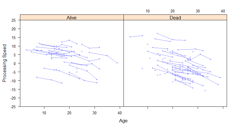
Figure 1: Subject-specific longitudinal trajectories of PS cognitive performance for $100$ randomly selected women in the MLSC database with and without an event.

4.2 MLSC Analysis Approach

We hypothesize that mortality may explicitly depend on previous PS trajectories, whereby individuals with lower scores and/or steeper trajectories should have a greater hazard of dying than those performing better. We also posit that, given the PS-mortality association, adequate description of cognitive change in adult individuals should statistically take into account their (future) mortality information. A previous survival analysis of these data showed that the proportional hazards assumption was not met when comparing mortality risk for male and female participants (aichele2015life). Therefore, sex-specific analyses are warranted. For simplicity, we limit the current analyses to data from female MLSC participants. Before estimating the joint model, we perform initial model selection steps independently for the longitudinal and for the time-to-event submodels.

We first select a submodel for the longitudinal part of the data. Based on a previous literature search on the use of the mixed-effects model in cognitive aging research (ghisletta2019), we tested six submodels: the first with fixed and random-effects for the intercept and the linear slope (to describe change over time), the second adding to the first a quadratic slope (change trajectories with a single curvature), the third adding to the second a cubic slope (change trajectories with two curvatures), and the fourth to the sixth with spline effects of time and with different numbers of nodes. Of the six submodels, based on statistical criteria, we choose the one that provides the most satisfying description of the PS trajectories.

We then, separately, select the optimal time-to-event submodel. To do so we rely on the Cox PH model that relates smoking status and initial age to the timing and occurrence of death. For each covariate we test the PH assumption and then retain the submodel that best describes the mortality process based on the selected covariates. Finally, we combine both submodels in joint modeling, and compare four association structures between the two submodels.

4.2.1 Longitudinal model selection

As required by the JMbayes package, we fit the longitudinal submodel with the lme($\cdot$) function from the nlme package (nlme). This longitudinal submodel must be specified in terms of its fixed and random components. For both components, linear and/or higher-degree polynomial terms are allowed (e.g., linear, quadratic or cubic change). More complex parameterizations of nonlinear effects are also feasible, such as achieved through the flexible spline methodology (see the second line in Equation (1) and cf. rizopoulos_book).

The spline approach has gain much popularity in recent years because of its flexibility in describing subject-specific longitudinal trajectories that follow highly nonlinear functions and that, individually, deviate from the average sample function. A spline is a piecewise function composed of polynomials adjusted to data within adjacent intervals, separated by equidistant points called nodes. The degree of the spline is defined by the polynomial of the highest degree used. For instance, if the function fitted to the data within an interval is a straight lines, the spline is said to be of degree $1$. Cubic splines are a popular specification for splines that entails polynomials of degree $3$ (hastie1987generalized). Within the lme($\cdot$) function, nonlinear effects can be specified with the subfunction ns($\cdot$) from the splines package. The ns($\cdot$) function uses natural cubic splines that estimate a smooth functions of the predictors (functions $f(\cdot)$ and $f_{i}(\cdot)$ in the second line of Equation (1); hastie_statistical_2017). With natural cubic splines, the data within each interval are fitted by a cubic spline, and splines from neighboring intervals must respect two conditions: at each node, the first and the second derivatives of the splines are continuous, meaning that, for any two adjacent intervals, the finishing portions of the left spline smoothly joins the starting portion of the right spline, thereby giving the visual impression of a single, continuos line passing through both intervals.

The user must select the optimal number of nodes, which is a rather arbitrary component of splines. However, this value should be less than or equal to the number of repeated measures. To this end, there is no automatic selection procedure implemented in the JMbayes package (in contrast to the mgcv package, for example; wood2006). We suggest to first investigate the number of nodes for the fixed part of the longitudinal submodel, before proceeding to explore that of random part (when both components are modeled using splines, as proposed in JMbayes). To do so we suggest testing multiple submodels with different number of nodes and comparing them on the basis of their Bayesian Information Criterion, where smaller values are preferable (BIC; schwarz1978estimating). The BIC is available in the lme($\cdot$) output and is known to penalize complex models more strongly than the Akaike Information Criterion (AIC; akaike_new_1974). Conveniently, the BIC allows a fully Bayesian interpretation (raftery_bayesian_1995). The difference in BIC between two models is to be interpreted as “not worth mentioning,” “positive,” “strong,” and “very strong” evidence against the model with highest value when the difference is between $0$ and $2$, $2$ and $6$, $6$ and $10$, and greater than $10$, respectively. (kass_raftery, p. 777). Applications of the spline-based approach within the joint modeling framework can be founded, for example, in rizopoulos2009fully, brown2005flexible, ding2008modeling, and rizopoulos2011bayesian.

As explained in oehlert2014few and pinheiro2000mixed, likelihood ratio tests to compare models with different fixed effects and same random effects should be performed using maximum likelihhod estimation (ML). However, the default estimation method implemented within the lme($\cdot$) function uses Restricted Maximum Likelihood (REML), because REML, unlike ML, produces unbiased estimates of variance and covariance parameters (the difference in bias vanishes with high number of observations). To meaningfully compare longitudinal submodels in terms of their BIC they should thus be re-estimated with ML.

For this illustration, we modeled change in cognitive performance as a function of age in years centered at age 50 (Age), conditioned on age in years at study entry (AgeStart). Thus, we add AgeStart and Age as fixed parameters to the longitudinal submodel. We also modeled Age as a random effect, because visually we might infer differences in rates of decline. Individual observed trajectories of PS are depicted in Figure 1.

We estimated the following specifications of the longitudinal submodel:

$$\begin{split}\texttt{lmeFit.mlsc1:}y_{i}(t)=&(\beta_{0}+b_{0{i}})+(\beta_{1}+b_{1{i}})\text{{Age}}_{i}(t)+\beta_{4}\text{{AgeStart}}_{i}+\epsilon_{i}(t),\\ \texttt{lmeFit.mlsc2:}y_{i}(t)=&(\beta_{0}+b_{0{i}})+(\beta_{1}+b_{1{i}})\text{{Age}}_{i}(t)+\beta_{2}\text{{Age}}_{i}(t)^{2}+\\ &\beta_{4}\text{{AgeStart}}_{i}+\epsilon_{i}(t),\\ \texttt{lmeFit.mlsc3:}y_{i}(t)=&(\beta_{0}+b_{0{i}})+(\beta_{1}+b_{1{i}})\text{{Age}}_{i}(t)+\beta_{2}\text{{Age}}_{i}(t)^{2}+\\ &\beta_{3}\text{{Age}}_{i}(t)^{3}+\beta_{4}\text{{AgeStart}}_{i}+\epsilon_{i}(t),\\ \texttt{lmeFit.mlsc4:}y_{i}(t)=&f(\text{{Age}}_{i}(t),2)+b_{0{i}}+b_{1{i}}\text{{Age}}_{i}(t)+\epsilon_{i}(t),\\ \texttt{lmeFit.mlsc5:}y_{i}(t)=&f(\text{{Age}}_{i}(t),3)+b_{0{i}}+b_{1{i}}\text{{Age}}_{i}(t)+\epsilon_{i}(t),\\ \texttt{lmeFit.mlsc6:}y_{i}(t)=&f(\text{{Age}}_{i}(t),4)+b_{0{i}}+b_{1{i}}\text{{Age}}_{i}(t)+\epsilon_{i}(t).\end{split}$$ (8)

The first three (lmeFit.mlsc1, lmeFit.mlsc2, lmeFit.mlsc3) estimate, respectively, a polynomial of first, second, and third degree of Age, respectively, with random effects for the intercept and Age. Models 4, 5, 6 (lmeFit.mlsc4, lmeFit.mlsc5 lmeFit.mlsc6) estimate cubic spline effects of Age with, respectively, 2, 3 and 4 nodes. Here, too, we included random effects for the intercept and Age. To do so, we used the R code in Section Code 2 lines 3-16 in the Computer Code Section.

We evaluated the adjustments of the six submodels in terms of their respective BIC values. The R code to this end can be founded in Section Code 2 lines 19-25 in the Computer Code Section. The results are displayed in Table 1.

	df	BIC
m1	7	29414.87
m2	8	29158.73
m3	9	29167.24
m4	8	29162.86
m5	9	29170.97
m6	10	29178.68
m2.1	9	29155.24
m2.2	10	29163.72

Table 1: BIC values for mixed-effects model comparisons.

For this we concluded that the submodel with a degree-2 polynomial for the fixed effects of Age and with a random intercept and a random Age slope fit the data best (m2, corresponding to lmeFit.mlsc2).

We subsequently expanded this submodel by adding interaction effects between the degree-2 Age polynomial and AgeStart, as shown in Equation (9). We again evaluated statistical fit with the BIC. The corresponding R code can be founded in Section Code 3 lines 1-4 in the Computer Code Section.

$$\begin{split}\texttt{lmeFit.mlsc2.1:}y_{i}(t)=&(\beta_{0}+b_{0{i}})+(\beta_{1}+b_{1{i}})\text{{Age}}_{i}(t)+\beta_{2}\text{{Age}}_{i}(t)^{2}+\\ &\beta_{3}\text{{AgeStart}}_{i}+\beta_{4}\text{{AgeStart}}_{i}\times\text{{Age}}_{i}(t)+\epsilon_{i}(t),\\ \texttt{lmeFit.mlsc2.2:}y_{i}(t)=&(\beta_{0}+b_{0{i}})+(\beta_{1}+b_{1{i}})\text{{Age}}_{i}(t)+\beta_{2}\text{{Age}}_{i}(t)^{2}+\\ &\beta_{3}\text{{AgeStart}}_{i}+\beta_{4}\text{{AgeStart}}_{i}\times\text{{Age}}_{i}(t)\\ &+\beta_{5}\text{{AgeStart}}_{i}\times\text{{Age}}_{i}(t)^{2}+\epsilon_{i}(t).\end{split}$$ (9)

The comparison between these two submodels and the previous m2 submodel is also displayed in Table 1 and indicates that the submodel m2.1 (corresponding to lmeFit.mlsc2.1) best fit the data (the R code can be founded in Section Code 3 lines 7-10 in the Computer Code Section).

To conclude this section on the longitudinal submodel of the MLSC PS score, we retain submodel lmeFit.mlsc2.1, which will be joined to the upcoming time-to-event submodel in the final joint model. The function for the true value of PS $\mu_{i}(t)$ (where the observed PS score $y_{i}(t)=\mu_{i}(t)+\epsilon_{i}(t)$) is

$$\mu_{i}(t)= (\beta_{0}+b_{0{i}})+(\beta_{1}+b_{1{i}})\text{{Age}}_{i}(t)+\beta_{2}\text{{Age}}_{i}(t)^{2}+\beta_{3}\text{{AgeStart}}_{i}+\beta_{4}\text{{AgeStart}}_{i}\times\text{{Age}}_{i}(t).$$ (10)

4.2.2 Time-to-event model selection

As discussed previously, the Cox PH submodel, defined in Equation (2), is often the preferred choice to analyze time-to-event data, given it does not require the user to specify a parametric hazard function. The nonparametric specification of the baseline hazard function within the coxph($\cdot$) function in R uses a B-spline approach, but if desired, regression splines can instead be invoked by setting the baseHaz function argument accordingly. The number and the position of the nodes are automatically selected, but they can also be fixed via the lng.in.kn and the knots function arguments.

In this illustration we specified a nonparametric baseline hazard function within the Cox PH submodel, with factor Smoker (whether or not an individual was a smoker at study entry) as baseline variable, conditioned on age in years at study entry (AgeStart). The corresponding R code can be founded in Section Code 4 lines 1-2 in the Computer Code Section and results are displayed in Table 2. The results show that factor Smoker is significant ($p$-value < 0.001). The estimated coefficient means that being smoker at study entry is associated with a hazard ratio of $\exp(0.519)=1.680$. That is, being smoker at study entry increases the relative risk of death by $68$%, compared to a non-smoker at entry.

	coef	exp(coef)	se(coef)	z	P
Smoker	0.519	1.680	0.064	8.092	<0.001
AgeStart	0.099	1.104	0.004	-9.815	<0.001

Table 2: Parameter estimates from the Cox PH model.

An important (and often overlooked) assumption of the Cox PH model is that baseline hazard functions for model predictors are proportional (cox1972). In other words, survival curves for different strata of a given predictor (determined by the particular choices of values for the $\gamma$-variables), have hazard functions that are proportional over time. For example, if the model specifies sex (male vs. female) as a mortality predictor, it is assumed that the hazard functions for males and females are proportional.

The PH assumption can be checked statistically using the Schoenfeld Residuals Test (SRT), which evaluates independence between model residuals and the time variable (here Age). More precisely, SRT checks whether the correlation between the scaled residuals and the time variable differs significantly from zero. If so, the PH assumption is violated, because the residuals are related to time, meaning that the hazard changes in time.

SRT can be applied for each predictor individually and also globally (for the model with all predictors) using the function cox.zph($\cdot$) from the survival package. Table 3 displays the results of the SRT and the corresponding R code can be founded in Section Code 4 line 3 in the Computer Code Section.

	rho	chisq	P
Smoker	-0.068	8.38	0.004
AgeStart	0.061	6.34	0.012
GLOBAL	NA	15.81	<0.001

Table 3: Schoenfeld Residuals Test form the Cox PH model.

The results of the SRT indicate that the PH assumption does not hold for the factor Smoker and for AgeStart as a predictor ($p$-values $<.05$), nor for the whole submodel ($p$-value $<.05$). When the PH assumption is not met for a predictor of theoretical interest, a stratification procedure for that predictor is required (fox2002cox). This stratification procedure is supported within the coxph($\cdot$) function inside the JMbayes package. In our particular case, we should thus stratify the time-to-event analysis by smoker status, with two strata, smoker vs non smoker, and also initial age, with an arbitrary number of strata (e.g., 50-59, 60-69, $\ldots$, 91-99 years), where within each the PH assumption is met. For the sake of simplicity within this tutorial, we do not use the stratification procedure and maintain the variables Smoker and AgeStart in the Cox PH submodel, as though the PH assumption were met for both. Kaplan-Meier survival curves by Age by smoker status are depicted in Figure 2.

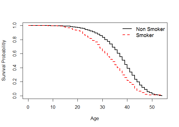
Figure 2: Kaplan-Meier estimator of survival probabilities for the two groups smokers versus non smokers.

4.2.3 Joint model

We are now ready to explore the association between longitudinal trajectories in processing speed and risk of death. We consider the three association structures as discussed above and, again, use a model comparison approach to select the final model.

The “current value” association

We start with the “current value” parameterization defined in Equation (4). For our data, this joint model si written as

$$\begin{split}h_{i}(t)=h_{0}(t)\exp\big{(}\beta_{1}\text{{Smoker}}_{i}+\beta_{2}\text{{AgeStart}}_{i}+\alpha_{1}\mu_{i}(t)\big{)},\end{split}$$ (11)

with $h_{0}(t)$ denoting the baseline hazard function. We estimated this submodel with the R command displayed in Section Code 5 lines 1-2 in the Computer Code Section. Note that the previously estimated longitudinal and time-to-event submodels are the main arguments of the jointModelBayes($\cdot$) function, and that the “current value” is the default association structure. The jointModelBayes($\cdot$) function uses a Metropolis-based Markov chain Monte Carlo (MCMC) algorithm, for which options must be chosen. We discuss these options in the Section Code 5 in the Computer Code Section.

Additionally, in a Bayesian paradigm, prior distributions must be specified for model parameters. A basic approach is to simply select non-informative priors, which is the default for JMbayes. If desired, informative prior distributions can also be specified. For example, in andrinopoulou2016bayesian, where the goal was to estimate elaborate models with many predictors in the time-to-event submodel, shrinkage priors were used in order to force small effects to be equal to zero while maintaining true large effects (VANERP201931). Of importance, JMbayes uses parameter estimates from the individual longitudinal and time-to-event submodels, as illustrated above, as starting values for the MCMC estimation of the joint model. Also, the package relies on a single, long chain, rather than multiple parallel, short chains.

As usual, before interpreting the results, we should worry about the estimation quality of the model. Various diagnostic plots are available within JMbayes. The plot($\cdot$) function can be used to visually examine convergence of the jointModelBayes($\cdot$) MCMC estimation. The output includes trace plots, autocorrelation plots, and kernel density estimation plots. An example of these plots for the association parameter fitted within the joint model with current value parametrization can be founded in Figure 3.

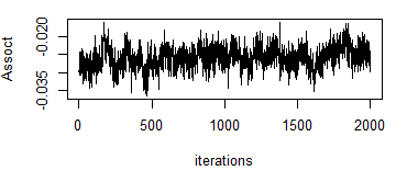
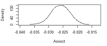
Figure 3: Trace plot, autocorrelation plot and kernel density plot for the associative parameter Assoct of the joint model with current value parametrization jointFit.mlsc1.

In the trace plots, we seek the so-called “lazy caterpillar” pattern, which means that across the various iterations the estimated values of the parameters are within reasonably restricted ranges, and are not suddenly outside such a range. For the autocorrelation plots, which represent the correlations between a solution and that a given lag from it, we seek autocorrelations that become small and as close to zero as quickly as possible (i.e., with small lags), meaning that the solutions of the simulated samples become quickly independent. The kernel density plots are smoothed histograms of the estimated solutions across the simulated samples. We expect these to be unimodal and with small tails. It is also possible to specify MCMC estimation with multiple shorter chains, which can also be diagnosed, but this requires additional R coding: Users must select different initial values within the priors space and then extract the corresponding MCMC output for analysis using the coda MCMC diagnostic package (coda; JMbayes).

The estimated parameter values can be obtained with the standard summary($\cdot$) function (line 4 of the Section Code 5 in the Computer Code Section). We show the results of this first association structure in Table 4. We report the posterior means of all estimated parameters, with their 95% credible intervals. The Assoct coefficient in the output represents $\alpha_{1}$ in Equation (11) and estimates the association between the true processing speed score at time $t$ and the risk of death at that same time. We can interpret this parameter as follows: The percent reductions in mortality risk associated with the current true value of processing speed for women is calculated as $1-\text{HR}\times 100$, where HR is the hazard ratio corresponding to a one-unit difference in the current true value of processing speed $\mu_{i}(t)$. Thus, HR is calculated as $\exp(-0.026)=0.974$, which gives $1-0.974=0.026$, and translates to $2.6\%$ lower risk of death per one unit increase in the current true value of processing speed. The coefficient for smoker statuts (0.445) indicates a strong association with mortality, with a $\exp(0.445)$ = $1.560$-fold increase in risk of death in smokers, compared to non smokers.

	Value	2.5%	97.5%
Smoker	0.445	0.328	0.555
AgeStart	-0.048	-0.055	-0.038
Assoct	-0.026	-0.032	-0.020
tauBs	12.186	4.643	25.541
(Intercept)	8.806	6.506	11.060
Age	0.192	0.079	0.302
AgeStart	-0.054	-0.090	-0.018
I(Age2)	-0.007	-0.007	-0.006
Age:AgeStart	-0.005	-0.006	-0.003
$\sigma$	0.946	0.916	0.977
D[1, 1]	31.550	28.805	34.265
D[2, 1]	-0.320	-0.402	-0.229
D[2, 2]	0.078	0.073	0.084

Table 4: Parameter estimates and 95% credible intervals for the “current value” association. D[i, j] denotes the $ij$-element of the covariance matrix of the random effects. tauBs is a hyperparameter relative to the distribution of the baseline hazard function $h_{0}(t)$ and is typically not interpreted.

The “current value plus slope” association

This second association structure takes the form

$$\begin{split}h_{i}(t)=h_{0}(t)\exp\big{(}\beta_{1}\text{{Smoker}}_{i}+\beta_{2}\text{{AgeStart}}_{i}+\alpha_{1}\mu_{i}(t)+\alpha_{2}\mu_{i}^{{}^{\prime}}(t)\big{)},\end{split}$$ (12)

and specifies that the hazard of experiencing the event at time $t$ is now assumed to be associated both with the true value of processing speed at time $t$, $\mu_{i}(t)$, and its current rate of change (i.e., slope) at time $t$, noted $\mu_{i}^{{}^{\prime}}(t)$.

Recalling Equation (10), the temporal variable is Age. The derivative of Equation (10) with respect to the temporal variable Age can be written as

$$\mu_{i}^{{}^{\prime}}(t) =\frac{\partial\mu_{i}(t)}{\partial\text{{Age}}}$$ (13)

$$=\beta_{1}+b_{1{i}}+\beta_{2}(2\times\text{{Age}}_{i}(t))+\beta_{4}\text{{AgeStart}}_{i}.$$

The R code for specifying the derivative form of this linear submodel and for running the corresponding joint model can be found in the Computer Code Subsections 6 and 7.

We show the results of the “current value plus slope” parametrization in Table 5.

	Value	2.5%	97.5%
Smoker	0.424	0.315	0.573
AgeStart	-0.056	-0.066	-0.048
Assoct	0.001	-0.008	0.010
AssoctE	-1.600	-1.984	-1.243
tauBs	14.250	5.747	28.615
(Intercept)	8.502	6.232	10.765
Age	0.185	0.070	0.295
AgeStart	-0.049	-0.086	-0.012
I(Age2)	-0.007	-0.007	-0.006
Age:AgeStart	-0.005	-0.006	-0.003
$\sigma$	0.946	0.910	0.981
D[1, 1]	31.093	28.992	33.549
D[2, 1]	-0.301	-0.396	-0.216
D[2, 2]	0.079	0.073	0.085

Table 5: Parameter estimates and 95% credible intervals for the “current value plus slope” association. D[i, j] denotes the $ij$-element of the covariance matrix of the random effects. tauBs is a hyperparameter relative to the distribution of the baseline hazard function $h_{0}(t)$ and is typically not interpreted.

Assoct represents $\alpha_{1}$ and AssoctE represents $\alpha_{2}$ in Equation (6), and quantify, respectively, the association between the current true value and the current rate of change of processing speed and the relative risk of death. We obtain $\alpha_{1}=0.001$ and $\alpha_{2}=-1.600$, with the 95% credible interval of Assoct that contains 0, while that of AssoctE does not. Clearly, then, the rate of change in perceptual speed at a given time point is a much more important predictor of than the actual true value of speed at that same time point. The lower the rate of change, the greater the odds of dying.

To interpret the effect of AssoctE on the risk of death, we could proceed as usual, by relating it to a one-unit change. However, whereas a one-unit value is a meaningful comparison for the current true value of speed, it is excessively large for the rate of change. To show this, we plotted in Figure 4 the current true value $\mu(t)$ estimated from the previous joint model with the “current value” association (continuous line) and the current rate of change $\mu^{{}^{\prime}}(t)$ (dashed line) from the joint model “current value plus slope”, as a function of the Age variable. We can immediately see that whereas the current value changes over a large range (from almost 6 to -10), the rate of change varies much less (from about 0 to less than -1). Hence, whereas a one-unit change could be useful in interpreting the former effect, it is less so for the latter effect (it would result in a $(1-\exp(-1.600))\times 100=79.81\%$ reduction in mortality risk, which is simply huge). Coming back to Figure 4, we note that over an interval of $40$ years, the current true value decreases by $14.722$ points, whereas the rate of change decreases by only $0.535$ points. This translates to an average decrease over a 10-year period of $3.684$ for the current true value and $0.134$ for the rate of change, with associated percent reductions in mortality risk of $9.13\%$ (calculated as $(1-\exp(-0.026\times 3.684))\times 100$) and $19.3\%$ (calculated as $(1-\exp(-1.6\times 0.133))\times 100$), respectively. We believe this exercice to be most useful to properly interpret the effect sizes stemming from this model, because, typically, the range of the current true value is much larger than that of its rate of change.

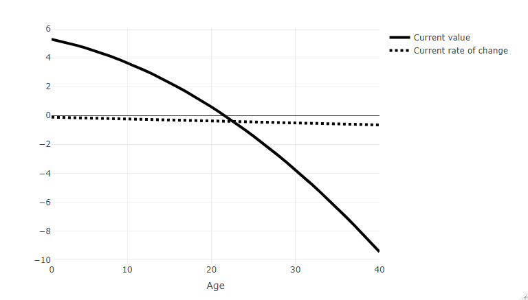
Figure 4: Average current value and average current rate of change (calculated without the random effects) for AgeStart fixed at its median value ($63$).

The “shared random effects” association

The third joint model can be written as

$$\begin{split}h_{i}(t)=h_{0}(t)\exp\big{(}\beta_{1}\text{{Smoker}}_{i}+\beta_{2}\text{{AgeStart}}_{i}+\alpha_{3}b_{0_{i}}+\alpha_{4}b_{1_{i}}\big{)},\end{split}$$ (14)

where $\alpha_{3}$ and $\alpha_{4}$ are the parameters of association of $b_{0i}$ and $b_{1i}$, which are defined in Equation (8) as the individual deviations from the sample average intercept and slope values, respectively. $\alpha_{3}$ and $\alpha_{4}$ define the association between the random intercept and the random slope effects, respectively, and the hazard of death. More precisely, for individuals having the same deviation from the average slope, the hazard ratio for a one-unit increase in individual deviation from the average intercept is $\exp(\alpha_{3})$. Conversely, for individuals having the same deviation from the average intercept, the hazard ratio for a one unit increase in individual deviation from the average slope is $\exp(\alpha_{4})$. The code for estimating the joint model with the “shared random effects” parameterization can be founded in Section Code 8 lines 1-3 in the Computer Code Section.

The results are displayed in Table 6. Assoct:(Intercept) represents $\alpha_{3}$ and Assoct:Age represents $\alpha_{4}$ in Equation (14). Subject-specific deviations from the sample average intercept are not predictive of the risk of death, whereas subject-specific deviations from the sample average slope are. To interpret this latter effect properly, rather than relating the reduction in mortality risk to a one-unit change, we relate it to a one-SD change, where D[2, 2]=0.080. This risk reduction is calculated as $1-\exp(\alpha_{4}\times\text{std}(b_{1}))=1-\exp(-1.641\times\sqrt{0.080})=0.371$. Thus, for a 1SD decrease in slope, the percent increase in mortality risk is $37.1\%$. Participants with greater cognitive decline have greater odds of dying than those declining less.

	Value	2.5%	97.5%
Smoker	0.410	0.291	0.536
AgeStart	-0.048	-0.056	-0.041
Assoct:(Intercept)	0.004	-0.006	0.014
Assoct:Age	-1.641	-1.884	-1.397
tauBs	7.426	2.792	16.424
(Intercept)	8.330	6.050	10.515
Age	0.192	0.079	0.308
AgeStart	-0.046	-0.081	-0.009
I(Age2)	-0.007	-0.007	-0.007
Age:AgeStart	-0.005	-0.007	-0.003
$\sigma$	0.957	0.924	0.993
D[1, 1]	31.438	29.167	33.827
D[2, 1]	-0.322	-0.411	-0.224
D[2, 2]	0.080	0.074	0.085

Table 6: Parameter estimates and 95% credible intervals for the “shared random effects” association. D[i, j] denotes the $ij$-element of the covariance matrix of the random effects. tauBs is a hyperparameter relative to the distribution of the baseline hazard function $h_{0}(t)$ and is typically not interpreted.

Joint model with interaction

We have illustrated the three association structures discussed previously in the joint models. Before reaching a final substantive conclusion about our data set, we would like to illustrate an additional extension of the association function $f(\cdot)$ in Equation (3). We illustrate interactions of predictors with the current true value $\mu_{i}(t)$ and/or current rate of change $\mu_{i}^{{}^{\prime}}(t)$ terms.

We illustrate this by extending the model jointFit.mslc1 to include an interaction term between the current true value of processing speed $\mu_{i}(t)$ and the smoker status. The corresponding time-to-event submodel can be written as

$$\begin{split}\begin{aligned} h_{i}(t)=&h_{0}(t)\exp\big{(}\beta_{1}\text{{Smoker}}_{i}+\beta_{2}\text{{AgeStart}}_{i}+\alpha_{1}\mu_{i}(t)+\alpha_{5}(\mu_{i}(t)\times\text{{Smoker}}_{i})\big{)},\end{aligned}\end{split}$$ (15)

where the interaction coefficient $\alpha_{5}$ expresses the difference in mortality prediction of $\mu_{i}(t)$ between smokers (Smoker = 1) compared to non-smokers (Smoker = 0).

The interaction is specified within the JMbayes package using the transFun argument, which takes as its value a generic function tf1 that, in turns, takes arguments x for the longitudinal parameter of interest and data for the predictor with which the longitudinal parameter interacts. This tf1 function has to be saved under its generic name (tf1) and defined in the workspace (see JMbayes, for more complex examples, such as multiple transformation functions applied simultaneously to multiple longitudinal parameters). The R code allowing one to write the generic function tf1 related to the submodel with interaction in Equation (15) can be founded in Section Code 9 line 1 in the Computer Code Section. The R code allowing one to source the function tf1 and to subsequently estimate the joint model with interaction can be founded in Section Code 9 lines 2-3 in the Computer Code Section.

The results are presented in Table 7. The coefficient Smoker means that being smoker (versus non-smoker) increases by 64.54% $(\exp(0.498)-1)\times 100)$ the risk of dying. Assoct ($\alpha_{1}$ in equation (15)) represents the association between the current true value of processing speed and the mortality risk and Assoct:Smoker ($\alpha_{5}$ in equation (15)) represents the interaction effect between the current true value of processing speed and the factor Smoker on the mortality risk. These results indicate that the current value of processing speed $\mu_{i}(t)$ is negatively associated with the risk of death (Assoct $=-0.028$). Going back to the previous interpretation of the Assoct effect of $3.684$ units over a 10-year period, rather than a one-unit change (cf. Figure 4), we obtain a $9.8\%$ (calculated as $(1-\exp(-0.028\times 3.684))\times 100$) increase in mortality risk. Note that this effect is very similar to the associative effect previously estimated for the “current value” parametrization, and remains different from zero. The interaction effect Assoct:Smoker is unimportant ($95\%$ credible interval contains 0), meaning that the effect of the current true value of processing speed on the mortality risk does not differ between smokers and non-smokers.

	Value	2.5%	97.5%
Smoker	0.498	0.306	0.667
AgeStart	-0.049	-0.057	-0.043
Assoct	-0.028	-0.034	-0.021
Assoct:Smoker	0.007	-0.007	0.020
tauBs	6.989	2.420	18.851
(Intercept)	8.746	6.453	11.048
Age	0.191	0.079	0.300
AgeStart	-0.054	-0.090	-0.016
I(Age2)	-0.007	-0.007	-0.006
Age:AgeStart	-0.005	-0.006	-0.003
$\sigma$	0.938	0.906	0.968
D[1, 1]	32.501	30.020	35.273
D[2, 1]	-0.346	-0.453	-0.241
D[2, 2]	0.079	0.073	0.084

Table 7: Parameter estimates and 95% credible intervals for the joint model with interaction. D[i, j] denotes the $ij$-element of the covariance matrix of the random effects. tauBs is a hyperparameter relative to the distribution of the baseline hazard function $h_{0}(t)$ and is typically not interpreted.

Model comparison

We can finally proceed to compare statistically the various association structures of the estimated joint models. To do so, we rely on the Deviance Information Criterion (DIC; Spiegelhalter), with smaller values indicating better model adjustments to the data. The R code computing the joint models comparison can be founded in Section Code 10 line 1 in the Computer Code Section. The results of joint models comparison can be founded in Table 8.

	df	LPML	DIC	pD
jointFit.mlsc1	5591	-26425.21	51793.14	5199.108
jointFit.mlsc2	5592	-26333.20	51606.23	5186.702
jointFit.mlsc3	5592	-26350.51	51791.15	5229.485
jointFit.mlsc4	5592	-26357.66	51773.84	5205.650

Table 8: Join models comparison.

LPML is the log-pseudo-marginal-likelihood value, DIC is the deviance information criterion and pD refers to the effective number of model parameters. Based on the DIC values, the evidence is strong to prefer the jointFit.mlsc2 model, which includes the current true value and the current rate of change of processing speed as predictors of the risk of death. Recall that within this model, the effect of the current true value in speed on the hazard of dying was not different from zero, whereas the association between the rate of change in speed and survival was strong. More precisely, individuals experiencing a greater rate of change, equivalent to what is expected over a 10-year interval, have a 19.3% greater mortality risk than those with shallower rates of change. Thus, we can conclude that cognitive performance per se, assessed via perceptual speed, does not relate strongly to mortality. Rather, it is the rate of change in cognitive performance that is predictive of survival, as hypothesized by the terminal decline and terminal drop hypotheses.

5 Discussion

In this tutorial, we presented an overview of the joint longitudinal and time-to-event modeling framework, presented a comparison of various R packages allowing this type of analysis, and illustrated how to use the most comprehensive of these R packages, JMbayes, to estimate a series of joint models. We illustrated joint models with real data from a psychological study on adult cognitive development and provided guidelines to choose among a series of theoretically motivated alternative specifications of joint models.

Due to space constraints and to limit complexity, we have not addressed other advanced features of the JMbayes package. These include functionalities for dynamic predictions, where survival probabilities can be estimated for a individual $i$ that was not part of the estimation sample, and for less common association structures. For instance, the package allows the “lagged effects” parametrization, where the hazard of experiencing the event at time $t$ is associated with the level of the longitudinal measure at a previous time point $t-p$, hence with a $p-$lag. For example, we might want to study how cognitive development during childhood might affect mortality later on in life. Thus, the longitudinal measures representing cognitive development during childhood at time $t-p$ could be related to mortality at time $t$, with an important (probably around 50-so years) lag $p$. An other association structure implemented in JMbayes is the “cumulative effects” parametrization, whereby the hazard of experiencing the event at time $t$ is associated with the whole information relative to the trajectory of the longitudinal measure up to time $t$. That is, rather than relating the value or slope on the true trajectory to the event, the whole surface under the trajectory constitutes the predictive information. For example, we might want to relate how learning characteristics during a critical period relate to mortality. In this case, performance during a given learning trial might be less informative or mortality than the entire learning history, as represented by the area under the learning curve.

Recently, JMbayes was extended to support simultaneous modeling of multiple longitudinal outcomes (using the function mvJointModelBayes($\cdot$)). This multiple parametrization may be useful when several longitudinal measures are recorded and may jointly impact the risk of death. For instance if several measure of cognitive development are recorded (as processing speed, fluid intelligence and crystallized intelligence in Rabbitt2004), they may jointly impact the risk of death. We also encourage interested readers to explore the developments of other R packages and other software allowing for joint model estimation.

The primary objective of this tutorial was to illustrate joint modeling of longitudinal and time-to-event data using the JMbayes package. Rather than reviewing the technical details of the joint modeling methodology, we aimed instead at providing researchers in behavioral sciences a practical understanding of what this powerful methodology can offer in substantive terms and how to apply it to their data. We hope this information will encourage adoption of the joint longitudinal-time-to-event modeling framework in research domains where it is currently underutilized and that should benefit from it.

6 Computer Code

6.1 Code 1

install.packages("JMbayes")
install.packages("rjags")
library(JMbayes)
library(rjags)

6.2 Code 2

ctrl <- lmeControl(opt="optim")

lmeFit.mlsc1 <- lme(FS_SPD ~  Age_50+AgeStart,
                    data = MLSC_fem2, random = ~ Age_50 | ID)
lmeFit.mlsc2 <- lme(FS_SPD ~  Age_50+I(Age_50^2)+AgeStart,
                    data = MLSC_fem2, random = ~ Age_50 | ID)
lmeFit.mlsc3 <- lme(FS_SPD ~  Age_50+I(Age_50^2)+I(Age_50^3)+AgeStart,
                    data = MLSC_fem2, random = ~ Age_50 | ID)


lmeFit.mlsc4 <- lme(FS_SPD ~  ns(Age_50,2)+AgeStart, data = MLSC_fem2,
                     random = ~ Age_50 | ID)
lmeFit.mlsc5 <- lme(FS_SPD ~  ns(Age_50,3)+AgeStart, data = MLSC_fem2,
                     random = ~ Age_50 | ID)
lmeFit.mlsc6 <- lme(FS_SPD ~  ns(Age_50,4)+AgeStart, data = MLSC_fem2,
                     random = ~ Age_50 | ID)


m1<-update(lmeFit.mlsc1, method = "ML" )
m2<-update(lmeFit.mlsc2, method = "ML" )
m3<-update(lmeFit.mlsc3, method = "ML" )

m4<-update(lmeFit.mlsc4, method = "ML" )
m5<-update(lmeFit.mlsc5, method = "ML" )
m6<-update(lmeFit.mlsc6, method = "ML" )

BIC(m1,m2,m3,m4,m5,m6)

ctrl <- lmeControl(opt="optim") changes the optimizer to be used for lme function (nlminb is the default).

6.3 Code 3

lmeFit.mlsc2.1 <- lme(FS_SPD ~  Age_50*AgeStart+I(Age_50^2),
                      data = MLSC_fem2, random = ~ Age_50 | ID)
lmeFit.mlsc2.2 <- lme(FS_SPD ~  Age_50*AgeStart+I(Age_50^2)*AgeStart,
                      data = MLSC_fem2, random = ~ Age_50 | ID)


m2.1<-update(lmeFit.mlsc2.1, method = "ML" )
m2.2<-update(lmeFit.mlsc2.2, method = "ML" )

BIC(m2,m2.1,m2.2)

6.4 Code 4

Coxfit_fem <- coxph(Surv(AgeLastObserved_2012_50, Dead_By2012) ~ Smoker+AgeStart,
                    data = MLSC_ID_fem2,x=TRUE)
print(cox.zph(Coxfit_fem))

In the joint modeling context we need to set x = TRUE (or equivalently model = TRUE) in the call of the coxph($\cdot$) function in order that the design matrix used in the Cox model is returned in the object fit (required for the joint model). Importantly, note that the scale of the temporal variable (here Age and AgeLastObserved_2012_50) should be identical in the longitudinal and in the survival models. The indicator for the event (alive or dead) is Dead_By2012.

6.5 Code 5

jointFit.mlsc1 <- jointModelBayes(lmeFit.mlsc2.1, Coxfit_fem,
                                  timeVar = "Age_50",n.iter = 30000)

summary(jointFit.mlsc1)

Call:
jointModelBayes(lmeObject = lmeFit.mlsc2.1, survObject = Coxfit_fem,
    timeVar = "Age_50", n.iter = 30000)

Data Descriptives:
Longitudinal Process Event Process
Number of Observations: 5517 Number of Events: 1858 (66.8%)
Number of subjects: 2780

Joint Model Summary:
Longitudinal Process: Linear mixed-effects model
Event Process: Relative risk model with penalized-spline-approximated
baseline risk function
Parameterization: Time-dependent value

      LPML      DIC       pD
 -26425.21 51793.14 5199.108

Variance Components:
             StdDev    Corr
(Intercept)  5.6169  (Intr)
Age_50       0.2801 -0.2035
Residual     0.9464

Coefficients:
Longitudinal Process
                  Value Std.Err Std.Dev    2.5%   97.5%      P
(Intercept)      8.8057  0.1290  1.1708  6.5061 11.0604 <0.001
Age_50           0.1922  0.0040  0.0574  0.0786  0.3024  0.001
AgeStart        -0.0542  0.0023  0.0189 -0.0899 -0.0176  0.002
I(Age_50^2)     -0.0066  0.0000  0.0002 -0.0069 -0.0063 <0.001
Age_50:AgeStart -0.0048  0.0001  0.0009 -0.0065 -0.0030 <0.001

Event Process
             Value Std.Err Std.Dev    2.5%   97.5%      P
SmokerTRUE  0.4449  0.0077  0.0567  0.3280  0.5549 <0.001
AgeStart   -0.0480  0.0010  0.0044 -0.0552 -0.0380 <0.001
Assoct     -0.0259  0.0003  0.0031 -0.0321 -0.0199 <0.001
tauBs      12.1863  1.2287  5.4554  4.6427 25.5413     NA

MCMC summary:
iterations: 30000
adapt: 3000
burn-in: 3000
thinning: 15
time: 17.6 min

lmeFit.mlsc2.1 is the longitudinal submodel, Coxfit_fem is the survival Cox submodel and timeVar = "Age_50" means that the temporal variable is Age_50. Note that no specification of the association structure is necessary, because the “current value” parameterization is the default implementation. Here we specified that, after the burn-in period, the MCMC algorithm should run for $30000$ iterations.

6.6 Code 6

dForm <- list(fixed= ~1 + I(2*Age_50) +AgeStart ,
              random = ~ 1, indFixed = c(2,4,5), indRandom = 2)

This R code means that the derivative of the current value ($\mu_{i}(t)$), with respect to Age_50, is equal for the fixed part (fixed=) to an intercept plus $2$ times the Age_50 variable plus AgeStart ($\beta_{1}+\beta_{2}(2\times\text{Age}_{i}(t))+\beta_{4}\text{AgeStart}$ in Equation (13)). The derivative of the random part of the model in Equation (13), with respect to Age_50, equals an intercept ($b_{1}$ in Equation (13)).

Arguments indFixed=c(2,4,5) and indRandom=2 refer to indices of the fixed and random model parameters corresponding to the retained (non-zero) arguments in the derivative of Equation (13). Thus, for the fixed parameters, indices c(2,4,5) relate to row numbers in the output of summary(jointFit.mslc1) under Longitudinal Process that correspond to the appropriate fixed model parameters $\{\beta_{1},\beta_{2},\beta_{4}\}$ (Section Code 5, lines 31-37). Similarly, for the random parameters, index 2 relates to row number relative to the random parameter $b_{1_{i}}$, found under Variance Components (Section Code 5, lines 24-28).

6.7 Code 7

jointFit.mlsc2 <- update(jointFit.mlsc1, param = "td-both", extraForm = dForm)

6.8 Code 8

jointFit.mlsc3<- jointModelBayes(lmeFit.mlsc2.1, Coxfit_fem,
                                 timeVar = "Age_50",param = "shared-RE",
                                 n.iter = 30000)

6.9 Code 9

tf1<-function (x, data) cbind(x, "Smoker" = x * (data$Smoker==’TRUE’))
jointFit.mlsc4 <- update(jointFit.mlsc1, transFun = tf1)

This tf1 function has to be saved under its generic name (tf1) in a separate R file and defined in the workspace. In this code, jointFit.mlsc4 calls jointFit.mlsc1 (the joint model with the current value parametrization) and the function tf1. It means that jointFit.mlsc4 will look for arguments x and data in the previously estimated model jointFit.mlsc1. x is the association structure used in jointFit.mlsc1 (here the current value $\mu_{i}(t)$) and data are the data used in the estimation of jointFit.mlsc1. Then, the function {cbind(x, "Smoker" = x * (data$Smoker==’TRUE’))} defines the columns of the design matrix $X_{i}(t)$ relative to the association structure (see Equation (1)). Here {cbind(x, "Smoker" = x * (data$Smoker==’TRUE’))} means that we will estimate first an simple effect of $\mu_{i}(t)$ (x), and then an interaction between the current value $\mu_{i}(t)$ and the factor Smoker ("Smoker" = x * (data$Smoker==’TRUE’))).

6.10 Code 10

anova(jointFit.mlsc1,jointFit.mlsc2,jointFit.mlsc3,jointFit.mlsc4)