Critical exponents and fine-grid vortex model of the dynamic vortex Mott transition in superconducting arrays.

Abstract

We study the dynamic vortex Mott transition in two-dimensional superconducting arrays in a magnetic field with $f$ flux quantum per plaquette. The transition is induced by external driving current and thermal fluctuations near rational vortex densities set by the value of $f$, and has been observed experimentally from the scaling behavior of the differential resistivity. Recently, numerical simulations of interacting vortex models have demonstrated this behavior only near fractional $f$. A fine-grid vortex model is introduced, which allows to consider both the cases of fractional and integer $f$. The critical behavior is determined from a scaling analysis of the current-voltage relation and voltage correlations near the transition, and by Monte Carlo simulations. The critical exponents for the transition near $f=1/2$ are consistent with the experimental observations and previous numerical results from a standard vortex model. The same scaling behavior is obtained for $f=1$, in agreement with experiments. However, the estimated correlation-length exponent indicates that even at integer $f$, the critical behavior is not of mean-field type.

I Introduction

Superconducting arrays provide an interesting testing ground for equilibrium and nonequilibrium phase transitions. They can be realized as two-dimensional (2D) arrays of coupled superconducting regions or “grains’, with well controlled parameters, being useful model systems of inhomogeneous superconductors, when phase fluctuations of the superconducting order parameter play a major role Newrock et al. (2000); Forrester et al. (1988); Geerligs et al. (1989); van der Zant et al. (1992); Ling et al. (1996); Baturina et al. (2011); Nguyen et al. (2016)

Recently, remarkable nonequilibrium phase transitions induced by an applied current, have been revealed through experiments on a square array of superconducting islands coupled by the proximity effect on a metallic film, in a perpendicular magnetic field Poccia et al. (2015); Lankhorst et al. (2018). The signature of the transition appears in the behavior of the differential resistivity at low temperatures, showing reversal of a minimum in to a maximum near certain values of the vortex density for increasing driving currents, and a corresponding scaling behavior as a function of current and vortex density near the transition. The transition has been identified as a classical analog of the dynamic quantum Mott insulator transition Nelson and Vinokur (1993); Tripathi et al. (2016); Li et al. (2015); Sankar and Tripathi (2019), with vortices playing the role of quantum particles. Dynamic vortex Mott transitions were clearly identified near integer vortex density $f=1$ and fractional vortex density $f=1/2$. The simplest model for such superconducting system consists of an ideal Josephson-junction array in an external magnetic field Teitel and Jayaprakash (1983); Granato (2018) on the same lattice as the superconducting grains, where logarithmically interacting vortices are located at plaquette centers, which act as pinning sites. The average vortex density corresponds to the frustration parameter $f$, defined as the number of flux quantum per plaquette. The scaling behavior of the differential resistivity observed experimentally Poccia et al. (2015); Lankhorst et al. (2018) was found to be described by a single critical exponent $\epsilon$. This behavior has been demonstrated in recent numerical simulations of interacting vortex models Rademaker et al. (2017); Granato (2018) only near fractional $f$. Outstandingly, for integer $f$, the value $\epsilon=2/3$ found experimentally agrees with a mean field description of the nonequilibrium dynamics obtained by mapping the dynamic vortex Mott transition into a non-Hermitian quantum problem Tripathi et al. (2016). Nevertheless, to characterize the critical behavior, the dynamic critical exponents $z$ and correlation-length exponent $\nu$ are also required. Near $f=1/2$, a different critical exponent $\epsilon=1/2$ was observed Poccia et al. (2015), which is not consistent with this mapping. Numerical results Granato (2018) for $f=1/2$, obtained from simulations of logarithmically interacting vortices, found an exponent $\epsilon$ consistent with the experimental observations and also obtained an estimate of the dynamic exponent $z\sim 2$ and correlation-length exponent $\nu\sim 1$. These critical exponents clearly indicate that the dynamic vortex Mott transition at fractional vortex densities belong to a different universality class. To fully characterize the transition for integer $f$, it should, therefore, be of interest to have similar information on the value of these critical exponents but, so far, there are no estimates available from experiments or numerical simulations for this case.

In this work, we study the dynamic vortex Mott transition in superconducting arrays using a lattice model of logarithmic interacting vortices, both at fractional and integer $f$. Because in the standard vortex model on a periodic lattice Teitel and Jayaprakash (1983); Granato (2018), the properties at integer $f$ are equivalent to $f=0$, it does not allow the study of this dynamic transition at nonzero integer vortex densities. To circumvent this problem, a fine-grid vortex model is introduced, allowing us to consider both the cases of fractional and integer $f$ while still keeping the simplicity of the original model. The critical behavior is determined from a scaling analysis of the current-voltage relation and voltage correlation near the transition, and by Monte Carlo simulations. We find that, for $f=1/2$, the dynamic transition is accompanied by a structural transition of the sliding vortex lattice. The critical exponent $\epsilon$ for $f=1/2$ is consistent with the experimental observations Poccia et al. (2015) and previous numerical results from the standard vortex model Granato (2018). The same scaling behavior of the differential resistivity is obtained for $f=1$, in agreement with experiments Poccia et al. (2015); Lankhorst et al. (2018). From the scaling analysis we find $\epsilon=1/2\nu$ and using the experimental results for $\epsilon$ we then conjecture the values $\nu=1$, $z=2$ for $f=1/2$ and $\nu=3/4$, $z=7/3$ for $f=1$, which are consistent with the numerical results within the errorbars. The results indicate that even for integer $f$ the dynamic vortex Mott transition is not of mean-field type and, therefore, fluctuations should be taken into account to fully describe the critical behavior.

II Model and simulation

In the standard vortex model of a 2D superconducting array, vortices can only be located at the centers of plaquettes of the lattice formed by the superconducting grains, which act as pinning sites. The grid of available sites correspond to the dual lattice of the array. The vortex Hamiltonian is given by Teitel and Jayaprakash (1983)

$$H_{v}=2\pi^{2}E_{o}\sum_{i,j}(n_{i}-f)G^{\prime}_{i,j}(n_{j}-f),$$ (1)

where vortices are represented by integer charges $n_{i}$ ($n_{i}=0,\pm 1...$) at the sites $r_{i}=(x_{i},y_{i})$ of the dual lattice, constrained by the neutrality condition, $\sum_{i}(n_{i}-f)=0$. $f$ is the number of flux quantum $\phi_{0}=hc/2e$ per plaquette of area $S$ introduced by the external magnetic field $B$, $f=BS/\phi_{0}$, and its value sets the average density of vortices. This vortex representation can be obtained following a standard procedure José et al. (1977) in which the usual Josephson-junction array model Teitel and Jayaprakash (1983), in terms of the phases of the local superconducting order parameter and Josephson coupling $E_{0}$, is replaced by a periodic Gaussian model, leading to explicit vortex variables $n_{i}$. The vortex interaction is given by $G^{\prime}_{ij}=G(r_{i}-r_{j})-G(0)$, where $G(r)$ is the lattice Green’s function Franz and Teitel (1995); Lee and Teitel (1994); Hyman et al. (1995). $G^{\prime}(\bf r)$ diverges logarithmically as $-\log(r)/(2\pi)$ for large separations. For a square lattice,

$$G({\bf r})=\frac{1}{L^{2}}\sum_{k}\frac{e^{i{\bf k}\cdot{\bf r}}}{4-2\cos({\bf k}\cdot{\bf a_{1}})-2\cos({\bf k}\cdot{\bf a_{2}})},$$ (2)

where $L$ is the system size, $\bf k$ are the reciprocal lattice vectors and $\bf a_{1}$, $\bf a_{2}$ are two perpendicular nearest-neighbor lattice vectors. When $f$ is an integer, a global change of the vortex charges $n_{i}\rightarrow n_{i}+f$, shows that the properties of the model are the same as the case without external field, $f=0$. Because of this periodicity in $f$, the standard model does not discriminate between zero and nonzero integer vortex densities, although it describes this transition for fractional vortex densities Granato (2018).

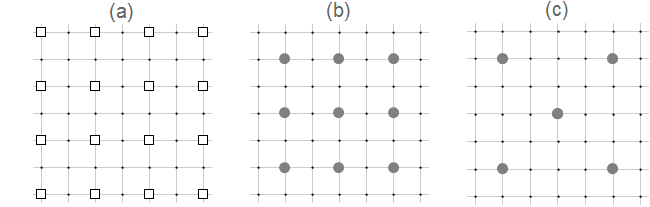
Figure 1: (a) Schematic of the fine-grid vortex model. Squares represent superconducting grains and grid points the allowed positions for vortices; (b) and (c) represent the vortex configurations (filled circles) in the ground state for $f=1$ and $f=1/2$, respectively.

In order to study both fractional and integer vortex densities within the same model, we introduce here a fine-grid vortex model on a square lattice. In addition to be located at the pinning sites of the array, vortices can now also be located at the junctions and at the grains of the array with a corresponding energy penalty (Fig. 1). The spacing of the grid of available sites is one half of the array spacing. The Hamiltonian of the fine-grid vortex model is given by

$$H_{fgv}=2\pi^{2}E_{o}\sum_{i,j}(n_{i}-f^{\prime})G^{\prime}_{i,j}(n_{j}-f^{\prime})+\sum_{i}E_{i}n_{i}^{2},$$ (3)

where the vortex charges $n_{i}$ are defined on the sites $r_{i}=(x_{i},y_{i})$ of the fine-grid lattice, constrained by the neutrality condition, $\sum_{i}(n_{i}-f^{\prime})=0$, where $f^{\prime}=f/4$. $E_{i}$ are additional vortex core energies: $E_{i}=E_{J}$ at the midpoint of the junctions between grains, $E_{i}=E_{G}>>E_{J}$ at the grains sites and $E_{i}=0$ at the pinning sites (plaquette centers). For sufficiently large $E_{J}$, the low-energy minimum for $f=1$ (Fig. 1b) corresponds to a vortex configuration where there is one vortex at each pinning site and for $f=1/2$ (Fig. 1c), there is one vortex at alternating pinning sites.

We study the nonequilibrium response of the superconducting array under an applied driving current by driven Monte Carlo (MC) simulations Lee and Teitel (1994); Hyman et al. (1995); Granato and Kosterlitz (1998); Granato (1998) of the fine-grid vortex model. The vortex dynamics is assumed to be overdamped. An external force is included, representing the effect of the driving current density $J$ on the vortices, acting as a Lorentz force transverse to the velocity, leading to an additional contribution to the energy in Eq. (3), $-(h/2e)J\sum_{i}n_{i}x_{i}$, when $J$ is in the $\hat{y}$ direction. The MC time is identified as the real time $t$ with the unit of time $dt=1$, corresponding to a complete MC pass through the lattice. A MC step consists of adding a dipole of vortex charges to a nearest-neighbor charge pair $(n_{i},n_{j})$, using the Metropolis algorithm. Choosing this charge pair at random, the step consists of changing $n_{i}\rightarrow n_{i}-1$ and $n_{j}\rightarrow n_{j}+1$, corresponding to the motion of a unit charge from $r_{i}$ to $r_{j}$. The move is accepted with probability $min[1,\exp(-\Delta H/kT)]$, where $\Delta H$ is the change in the energy. Periodic boundary conditions are used in systems of linear size $L$. The driving current $J$ biases the added dipole, leading to a net flow of vortices in the direction transverse to the current, if the vortices are mobile. This vortex flow generates an electric field $E$ along the current which can be calculated (in arbitrary units) as $E(t)=\frac{1}{L}\sum_{i}\Delta Q_{i}(t)$, after each MC pass through the lattice, where $\Delta Q_{i}=({\bf r_{i}}-{\bf r_{j}})\cdot{\bf\hat{x}}$ for an accepted vortex dipole excitation at the sites $(i,j)$ and $\Delta Q_{i}=0$ otherwise. Due to the neutrality condition, $f^{\prime}$ is varied in multiples of $1/L^{2}$. Temperature $T$ is measured in units of $E_{o}/k_{B}$ and $J$ in units of $(2e/h)E_{o}$.

The results of the simulations presented in Sec. IV are for $E_{J}/E_{0}=2$ with $E_{G}=4E_{J}$. We use typically $5\times 10^{5}$ MC passes to compute time averages and the same number of passes to reach steady states.

III Scaling analysis

The expected behavior of the differential resistivity and other measurable quantities follows from general arguments of the scaling theory of a continuous dynamic transition occurring at a critical current $J_{c}$. Measurable quantities should scale with the diverging correlation length $\xi\sim|\delta J|^{-\nu}$ and relaxation time $\tau\sim\xi^{z}$, where $\delta J=J-J_{c}$, and $\nu$ and $z$ are the correlation length and dynamic critical exponents, respectively. In particular, the differential resistivity scaling can be obtained in a similar manner as for the current-voltage scaling of inhomogeneous superconductors Fisher et al. (1991); Hyman et al. (1995), adapted to the present case of a transition at the critical current $J_{c}$ and frustration $f_{c}$, with nonzero vortex density.

III.1 Current-voltage relation and differential resistivity

Since the electric field $E$ generated by moving vortices with density $f$ and velocity $v$ is proportional to $fv$, the singular contribution to $E$ should scale as $E\sim\xi^{1-z}$. Crossover effects due to a change $\delta f=f-f_{c}$ should occur when $|\delta f|\xi^{2}\approx 1$, corresponding to an additional vortex in a correlated area, revealing that $\delta f$ is a strongly relevant perturbation and should therefore appear in the scaling function in the combination $\delta J/|\delta f|^{1/2\nu}$. As a function of $\delta J$ and $\delta f$, one then expect the current-voltage scaling Granato (2018)

$$E(J,f)=F_{o}(J,f)+|\delta f|^{\beta\epsilon}F_{1}(\delta J/|\delta f|^{\epsilon}),$$ (4)

where $F_{o}$ is a regular contribution, analytic in $\delta J$ and $\delta f$, and $F_{1}(x)$ is a scaling function with $F_{1}(0)=c$, a constant. The exponents $\beta$ and $\epsilon$ are determined by the correlation length and dynamic critical exponents as

$$\beta = (z-1)\nu,$$ (5)

$$\ \epsilon = 1/2\nu.$$ (6)

The scaling form for the differential resistivity $dE/dJ$ can then be obtained from Eq. (4) as

$$\frac{dE(J,f)}{dJ}-\frac{dE(J,f)}{dJ}|_{J=J_{c}}=|\delta f|^{(\beta-1)\epsilon}H(\delta J/|\delta f|^{\epsilon}),$$ (7)

with $H(0)=0$. We have neglected the $\delta J$ dependence of $dF_{o}(J,f)/dJ$.

The above scaling form reduces to the one used in the experiments Poccia et al. (2015); Lankhorst et al. (2018) when $\beta=1$,

$$\frac{dE(J,f)}{dJ}-\frac{dE(J,f)}{dJ}|_{J=J_{c}}=H(\delta J/|\delta f|^{\epsilon}),$$ (8)

which depends on a single exponent, $\epsilon$. The experimental data for the differential resistivity is well described by this scaling form, both for fractional and integer frustration $f$. However, to fully characterize the critical behavior, the critical exponents $z$ and $\nu$ are also required.

With $\beta=1$ and using the exponent relations in Eq. (5) we can conjecture the values of the other exponents $\epsilon$, $\nu$ and $z$, assuming one of them. The usual exponent for relaxation dynamics, $z=2$, implies that $\nu=1$, which leads to a crossover exponent $\epsilon=1/2\nu=0.5$. Remarkably, this value agrees with the experimental results Poccia et al. (2015) for $f=1/2$ and also with the numerical results from the standard vortex model Granato (2018). For $f=1$, however, the experiments find a different value Poccia et al. (2015); Lankhorst et al. (2018), $\epsilon=2/3$. Assuming this value for $\epsilon$, we get $\nu=3/4$ and $z=7/3$. In the next Section, we compare these conjectured values with the numerical results obtained with the present fine-grid vortex model.

III.2 Relaxation time

To determine the values of the critical exponents $z$ and $\nu$ from numerical simulations, we performed a scaling analysis of the relaxation time $\tau(J,f)$, obtained from the voltage time correlation function

$$C(t)=\frac{<V(t)V(0)>-<V(t)>^{2}}{<V(t)^{2}>-<V(t)>^{2}}.$$ (9)

Near the transition, $\tau$ can be estimated from the expected time dependence of $C(t)$ at long times, $C(t)\propto e^{-t/\tau}$. Since $\epsilon=1/2\nu$, the relaxation time $\tau\sim\xi^{z}$ should then satisfy the scaling form

$$\tau|\delta f|^{z/2}=G(\delta J/|\delta f|^{1/2\nu}),$$ (10)

in the absence of finite-size effects. The critical exponents $\nu$ and $z$ can be estimated from the best data collapse in a plot of $\tau|\delta f|^{z/2}$ versus $\delta J/|\delta f|^{1/2\nu}$, satisfying this scaling form. To minimize the finite-size effects, this data collapse is performed for large systems and in a range of $f$ not too close to $f_{c}$.

However, when the correlation length $\xi$ becomes comparable to the system size $L$, the scaling function will also depend on the dimensionless ratio $L/\xi$ as

$$\tau|\delta f|^{z/2}=F_{2}(\delta J/|\delta f|^{1/2\nu},\delta JL^{1/\nu}).$$ (11)

This makes the numerical determination of the critical parameters very complicated due to the presence of two scaling variables. As a simplification, in this case we consider data at current densities and system sizes such that $\delta JL^{1/\nu}$ is equal to a constant value. Then, the scaling function $F_{2}$ depends only on a single variable $\delta J/|\delta f|^{1/2\nu}$.

At the transition, $J=J_{c}$, the correlation length is cutoff by the system size $L$ and the relaxation time $\tau$ should satisfy the finite-size scaling form

$$\tau/L^{z}=F_{3}(L^{2}|\delta f|).$$ (12)

III.3 Vortex correlation

The dynamic vortex Mott transition should correlate with a change in the structure of the sliding state of the vortex lattice. For $f=1/2$, we find that this change can be quantified from the behavior of the structure factor $S({\bf k})$, which is a measure of the vortex correlations,

$$S({\bf k})=\frac{1}{L^{2}}<|n({\bf k})|^{2}>,$$ (13)

where $n({\bf k})$ is the Fourier transform of the vortex variables $n_{i}$. The sliding ordered state below $J_{c}$ corresponds to sharp peaks in the structure factor $S({\bf k})$ at the wave vectors ${\bf k_{o}}$ of a periodic vortex structure. Above $J_{c}$, the peaks broaden and become very small corresponding to a disorder phase. Assuming a structural phase transition, $S({\bf k_{o}})$ should then satisfy the scaling form

$$S({\bf k_{o}})|\delta f|^{(1-\eta/2)}=F_{4}(\delta J/|\delta f|^{1/2\nu},\delta JL^{1/\nu}),$$ (14)

where $\eta$ is an additional critical exponent characterizing the power-law decay of vortex correlations at the transition $<n_{j}n_{l}\ e^{i{\bf k_{0}}\cdot({\bf r_{j}}-{\bf r_{l}})}>\sim|{\bf r_{j}}-{\bf r_{l}}|^{-\eta}$. At the transition, it should satisfy the scaling form

$$S({\bf k_{o}})/L^{(2-\eta)}=F_{5}(L^{2}|\delta f|).$$ (15)

We also consider the scaling behavior of the finite-size vortex correlation length, which can be obtained from $S(k)$ as

$$\xi(J,f)=\frac{1}{2\sin(k_{m}/2)}[S(k_{0})/S(k_{1})-1]^{1/2}.$$ (16)

Here ${\bf k_{1}}={\bf k_{0}}+{\bf k_{m}}$ and ${\bf k_{m}}$ is the smallest nonzero wave vector of the lattice. This expression is a generalization of the usual second-moment correlation length Amit and Martin-Mayor (2005) for an order parameter with nonzero wave vector $\bf k_{o}$. Above the transition, $J>J_{c}$, this definition corresponds to a finite-difference approximation to the infinite system correlation length $\xi^{2}=-\frac{1}{S({\bf k})}\frac{\partial S({\bf k})}{\partial({\bf k}-{\bf k_{0}})^{2}}|_{{\bf k}={\bf k_{0}}}$, taking into account the lattice periodicity. $\xi$ should satisfy the scaling form

$$\xi|\delta f|^{1/2}=F_{6}(\delta J/|\delta f|^{1/2\nu},\delta JL^{1/\nu}),$$ (17)

near the transition. At the transition, it should satisfy the scaling form

$$\xi/L=F_{7}(L^{2}|\delta f|),$$ (18)

which, interestingly enough, does not depend on the critical exponents. To verify the scaling behavior of Eqs. (14) and (17), we use the same procedure as for Eq. (11).

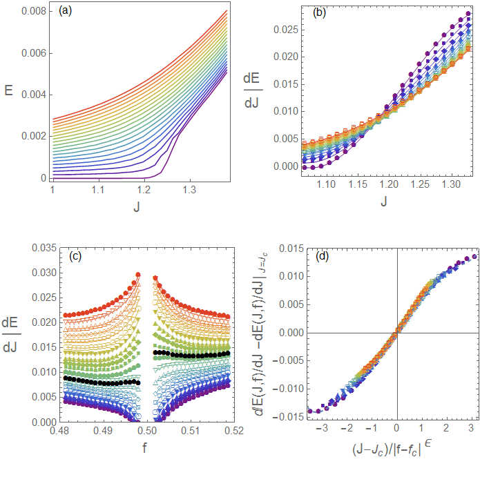
Figure 2: (a) Nonlinear current-voltage characteristics ($J=I/L$, $E=V/L$ ) for increasing frustration $f$ near $f=1/2$. Temperature $T=0.2$ and system size $L=64$. From the bottom up, $f$ increases from $0.5$ to $0.518555$ in $19$ equal steps. (b) Differential resistivity $\frac{dE}{dJ}$ for $f\geq 0.50293$ near the transition. (c) $\frac{dE}{dJ}$ as a function of $f$ for different $J$. From the bottom up, $J$ increases from $1.06552$ to $1.32759$ in $20$ equal steps. The separatrix $dE/dJ_{J=J_{c}}$ is indicated by black dots. (d) Scaling plot of $\frac{dE}{dJ}$ for $f>1/2$, with $J_{c}=1.203$, $f_{c}=0.5$ and $\epsilon=0.55$.

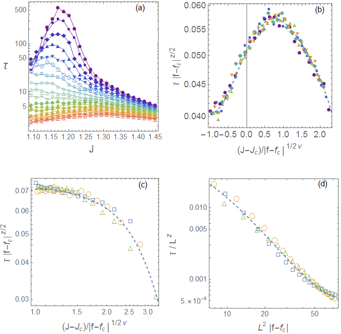
Figure 3: (a) Relaxation time $\tau(J,f)$ at different values of $f$, near the dynamical transition for $f=1/2$. Temperature $T=0.2$ and system size $L=112$. $f$ increases from $0.500957$ to $0.518176$ in $18$ equal steps; b) Scaling plot for $f\geq 0.514349$ neglecting finite-size effects with $J_{c}=1.19$, $f_{c}=0.501$, $\nu=1$ and $z=2$; (c) Scaling plot with $\delta JL^{1/\nu}=c$, a constant ($c=7.09$), with $J_{c}=1.16$, $f_{c}=0.501$, $\nu=1.1$ and $z=1.9$. Open squares correspond to $L=48$, circles to $L=64$ and triangles to $L=80$; (d) Scaling plot at $J_{c}=1.24$ with $z=2.1$.

IV Numerical simulations and discussion

IV.1 Fractional vortex density: $f=1/2$

First, we consider the dynamic vortex Mott transition near $f=1/2$ and check if the present fine-grid vortex model gives the same results as the previous simulations Granato (2018) with the standard vortex model. New results are also obtained from calculations of the vortex structure factor and correlation length. Figure 2a shows the effect of increasing the frustration $f$ from $f=1/2$ on the current-voltage (I-V) relation, in terms of the current density $J=I/L$ and the electric field $E=V/L$ at a temperature $T=0.2$. This temperature is well below the critical temperature of the equilibrium resistive transition, $T_{c}\sim 0.8$, which occurs at $J=0$. A small increment in $f$ from $f=1/2$ leads to an increase in the slope of the current-voltage curve, which changes sharply at a critical value $J_{c}\approx 1.2$. Further increase of $f$ tends to smooth out the slope of these curves near $J_{c}$. This change of slope near $J_{c}$ can been seen much clearer in the behavior of the differential resistivity, $dE/dJ$, shown in Fig. 2b. To obtain smooth curves for $dE/dJ$ by numerical differentiation, the current-voltage data in the small interval near $J_{c}$ was fitted to a low order polynomial. Fig. 2b reveals that the curves $dE/dJ\times J$ for different $f>0.502$ cross approximately at the same point $J_{c}$. The crossing point is a manifestation of the underlying dynamic transition, with $dE/dJ$ behaving approximately as a scaling invariant quantity and $f-f_{c}$ acting as a relevant perturbation Granato (2018), consistent with the scaling form of Eq. (7) when $\beta=1$. When the differential resistivity is plotted as a function of $f$ for different currents in Fig. 2c, where data for $f<1/2$ is also included, there is a characteristic reversal of a minimum into a maximum near $f=1/2$ for increasing current density, at $J_{c}$. The main difference of this behavior in the present model and the standard model Granato (2018) is the assymetry of the curves with respect to $f-1/2$. In Fig. 2d, we plot the data near the transition according to the scaling form of Eq. (8), originally proposed in the experiments Poccia et al. (2015). Data for different $J$ and $f$ collapse into the same smooth curve when $J_{c}$, $f_{c}$ and $\epsilon$ have the appropriate values. The value obtained for the critical exponent, $\epsilon=0.55(7)$, is consistent with the one obtained from previous numerical simulations with the standard model Granato (2018) and also with the experiments Poccia et al. (2015), supporting the universality of this dynamical transition. The reversal of the minimum in to a maximum and the data collapse characterized by a single exponent $\epsilon$ are the signatures of the dynamic vortex Mott transition as observed in the experiments Poccia et al. (2015); Lankhorst et al. (2018).

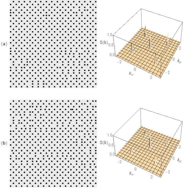
Figure 4: Snapshots of the vortex configurations and corresponding structure factor $S(\vec{k})$ at $J=1.17034$ (a) and $J=1.22276$ (b), below and above the dynamical transition, respectively, for $f=0.505859$.

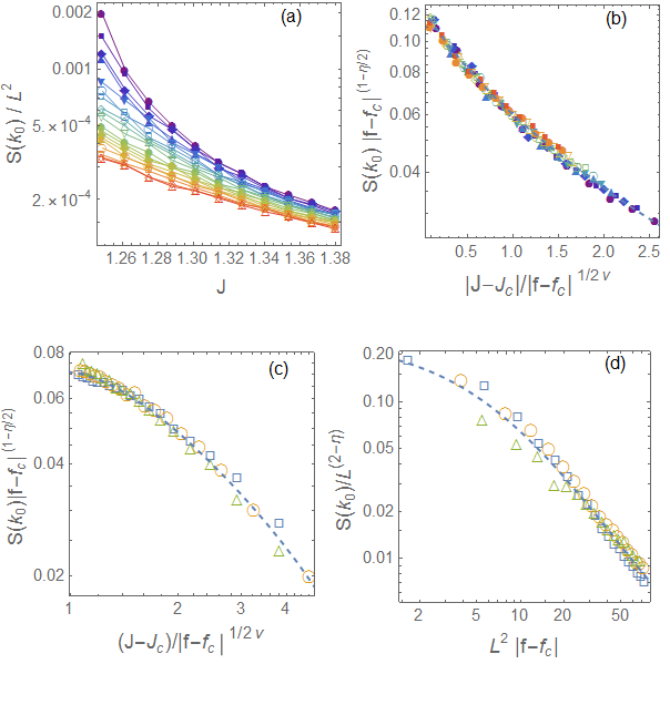
Figure 5: (a) Vortex structure factor peak $S(k_{0})$ at different values of $f$, near the dynamical transition for $f=1/2$. Temperature $T=0.2$ and system size $L=80$. $f$ increases from $0.501875$ to $0.511875$ in $17$ equal steps; (b) Scaling plot for $f\geq 0.505$ neglecting finite-size effects, with $J_{c}=1.24$, $\nu=0.95$ and $\eta=0.7$; (c) Scaling plot with $\delta JL^{1/\nu}=c$, a constant ($c=8.64$), with $J_{c}=1.23$, $f_{c}=0.501$, $\nu=1.0$ and $\eta=0.7$. Open squares correspond to $L=48$, circles to $L=64$ and triangles to $L=80$. (d) Scaling plot at $J_{c}=1.23$ with $f_{c}=0.501$ and $\eta=0.7$.

In Figs. 3a, we show the behavior of the relaxation time $\tau$ obtained from the voltage time correlation function, defined in Eq. (9), as a function of the driving current and different $f$ near $f=1/2$. A reasonable data collapse according to scaling forms of Eq. (11) (Figs. 3b and 3c) and Eq. (12) (Fig. 3d) is obtained with $z\approx 2$ and $\nu\approx 1$.

The dynamic vortex Mott transition correlates with a change in the structure of the sliding state of the vortex lattice. As can be seen from the snapshots of the vortex configuration in Fig. 4a and Fig. 4b, obtained below and above the critical current $J_{c}$, respectively, the vortex lattice remains essentially ordered below $J_{c}$ but has a large number of defects above $J_{c}$. The transition in the vortex structure can be determined from the behavior of the structure factor $S(\vec{k})$, defined in Eq. (13), which is a measure of the vortex correlations. The sliding ordered state below $J_{c}$ (Fig. 4a) corresponds to sharp peaks in the structure factor $S(\vec{k})$ at the wave vectors $\vec{k}_{o}$ of the periodic vortex structure, as expected for a commensurate frustration $f=1/2$. Above $J_{c}$ (Fig. 4b), the peaks broaden and become very small corresponding to the disordered phase. In Figs. 5a, we show the behavior of the structure factor peak $S(\vec{k}_{0})$ as a function of the driving current $J>J_{c}$ and different $f$, near $f=1/2$. As shown in Figs. 5b, 5c and 5d, a reasonable data collapse according to the scaling forms of Eq. (14) and Eq. (15) is obtained with $\nu\approx 1$, $\eta\approx 0.7$ and $J_{c}=1.23$. Finally, in Figs. 6a, we show the behavior of the vortex correlation length $\xi(J,f)$, defined in Eq. (16) with ${\bf k_{m}}=(2\pi/L){\bf\hat{x}}$, as a function of the driving current and different $f$ near $f=1/2$. A reasonable data collapse according to the scaling form of Eq. (17) (Figs. 6b and 6c) is obtained with $\nu\approx 1$ and Fig. 6d shows that the data collapse at $J_{c}$ is consistent with Eq. (18), which does not depend on the critical exponent $\nu$. These estimates of the exponents obtained from vortex correlations agree with the values obtained from the voltage time correlation showing that indeed the dynamic vortex Mott transition for $f=1/2$ corresponds to a structural phase transition of the sliding vortex lattice.

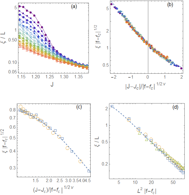
Figure 6: (a) Vortex correlation length $\xi(J,f)$ at different values of $f$, near the dynamical transition for $f=1/2$. Temperature $T=0.2$ and system size $L=80$. $f$ increases from $0.501875$ to $0.511875$ in $17$ equal steps; (b) Scaling plot for $f\geq 0.505$ neglecting finite-size effects, with $J_{c}=1.24$, $f_{c}=0.5015$ and $\nu=0.95$; (c) Scaling plot with $\delta JL^{1/\nu}=c$, a constant ($c=8.64$), with $J_{c}=1.20$, $f_{c}=0.501$ and $\nu=1.0$. Open squares correspond to $L=48$, circles to $L=64$ and triangles to $L=80$. (d) Scaling plot at $J_{c}=1.23$ with $f_{c}=0.501$.

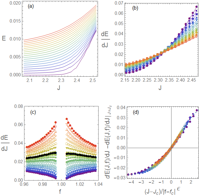
Figure 7: (a) Current-voltage characteristics for increasing frustration $f$, near $f=1$. Temperature $T=0.2$ and system size $L=64$. From the bottom up, $f$ increases from $1$ to $1.03711$ in $19$ equal steps. (b) differential resistivity $\frac{dE}{dJ}$ as a function of $J$ for $f\geq 1.00586$, near the transition. (c ) $\frac{dE}{dJ}$ as a function of $f$ for different $J$. From the bottom up, $J$ increases from $2.15517$ to $2.47241$ in $20$ equal steps. The separatrix $dE/dJ_{J=J_{c}}$ is indicated by black dots. (d) Scaling plot of $\frac{dE}{dJ}$ with $J_{c}=2.3534$, $f_{c}=1.0$ and $\epsilon=0.6$.

IV.2 Integer vortex density: $f=1$

We now consider the dynamic vortex Mott transition near an integer vortex density, $f=1$, and extract the critical exponents $\epsilon$, $\nu$ and $z$ from the expected scaling behavior as described in Sec. III. Figure 7a shows the effect of increasing the frustration $f$ from $f=1$ on the current-voltage relation at a temperature $T=0.2$. The corresponding behavior of the differential resistivity, $dE/dJ$, is shown in Fig. 7b. The differential-resistivity curves for different $f$ cross approximately at the same point $J_{c}\sim 2.3$ signaling the dynamic vortex Mott insulator transition. In Fig. 7c , $dE/dJ$ is plotted as a function of $f$ for different currents, where data for both $f<1$ and $f>1$ are included, showing the reversal of a minimum into a maximum near $f=1$ for increasing currents. The separatrix of the two regimes is indicated by the dotted lines. In Fig. 7d, we plot the data near the transition according to the scaling form of Eq. (8), giving an estimate of the critical exponent $\epsilon\approx 0.60(7)$. The characteristic minimum-maximum reversal of the differential resistivity near $f=1$ for increasing current and the corresponding data collapse are in good agreement with the behavior of the dynamic vortex Mott transition as observed in the experiments Poccia et al. (2015); Lankhorst et al. (2018) with $\epsilon=2/3$, supporting the universality of this dynamic transition.

In Figure 8a, we show the behavior of the relaxation time $\tau$ obtained from voltage time correlations as a function of the driving current and different $f$ near $f=1$. A reasonable data collapse according to the scaling forms of Eq. (11) (Fig. 8b and 8c ) and Eq. (12) (Fig. 8d) are obtained with $\nu\approx 0.70(7)$ and $z=2.40(7)$. The estimated values of $\nu$ and $z$ are indeed compatible with the conjectured values $\nu=3/4$ and $z=7/3$ inferred from the scaling analysis of Sec. IIIA

V Conclusions

We have considered the dynamic vortex Mott transition in 2D superconducting arrays in a magnetic field with $f$ flux quantum per plaquette. This nonequilibrium dynamic transition is induced by external driving current and thermal fluctuations near rational vortex densities set by the value of $f$. Experimentally, the transition has been determined from the scaling behavior of the differential resistivity characterized by a critical exponent $\epsilon$. Recent numerical simulations of interacting vortex models Granato (2018); Rademaker et al. (2017) have demonstrated this behavior only near fractional $f$. A fine-grid vortex model was introduced, which allowed us to consider both the cases of fractional and integer $f$, and investigate the critical behavior by a scaling analysis and MC simulations. For $f=1/2$, the dynamic transition is accompanied by a structural transition of the sliding vortex lattice. The critical exponents are consistent with the experimental observations Poccia et al. (2015), and previous numerical results from a standard vortex model Granato (2018). The same scaling behavior of the differential resistivity is obtained for $f=1$, in agreement with experiments Poccia et al. (2015); Lankhorst et al. (2018). However, we find a correlation-length exponent $\nu\sim 0.75$, which is significantly different from the one expected from mean-field theories, $\nu=1/2$. From the scaling analysis we find $\epsilon=1/2\nu$ and using the experimental results for $\epsilon$ we then conjecture the values $\nu=1$, $z=2$ for $f=1/2$ and $\nu=3/4$, $z=7/3$ for $f=1$, which are consistent with the numerical results within the errorbars Although the critical exponent $\epsilon=2/3$ observed experimentally for integer $f$ can be obtained at the mean-field level by mapping to a single particle non-Hermitian Hamiltonian Tripathi et al. (2016), our results indicate that the full critical behavior is not described by this approximation and fluctuations should be taken into account.

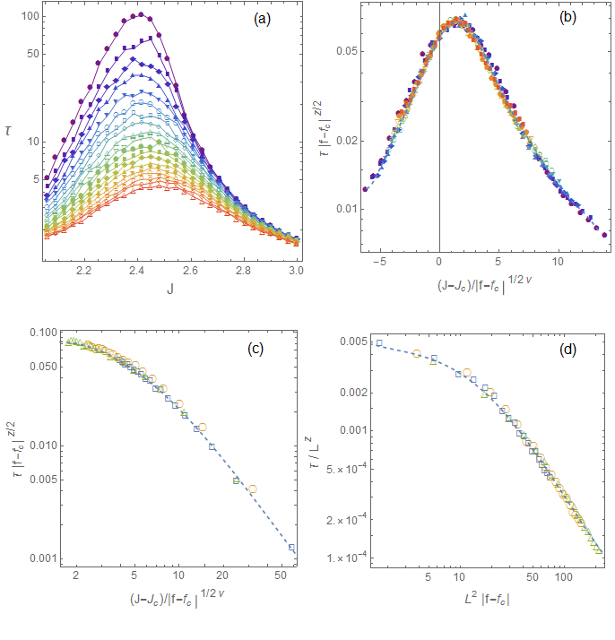
Figure 8: (a) Relaxation time $\tau(J,f)$ at different values of $f$, near the dynamical transition for $f=1$. Temperature $T=0.2$ and system size $L=80$. $f$ increases from $1.00188$ to $1.03563$ in $18$ equal steps; (b) Scaling plot for $f\geq 1.01563$ neglecting finite-size effects with $J_{c}=2.35$, $f_{c}=1.002$, $\nu=0.7$ and $z=2.5$; (c) Scaling plot with $\delta JL^{1/\nu}=c$, a constant ($c=85.75$), with $J_{c}=2.36$, $f_{c}=1.001$, $\nu=0.7$ and $z=2.4$. Open squares correspond to $L=48$, circles to $L=64$ and triangles to $L=80$; (d) Scaling plot at $J_{c}=2.36$ with $z=2.4$.

References

- Newrock et al. (2000) R. S. Newrock, C. J. Lobb, U. Geigenmüller, and M. Octavio, Solid State Physics 54, 263 (2000).
- Forrester et al. (1988) M. Forrester, H. J. Lee, M. Tinkham, and C. Lobb, Phys. Rev. B 37, 5966 (1988).
- Geerligs et al. (1989) L. J. Geerligs, M. Peters, L. E. M. de Groot, A. Verbruggen, and J. E. Mooij, Phys. Rev. Lett. 63, 326 (1989).
- van der Zant et al. (1992) H. S. J. van der Zant, L. J. Geerligs, and J. E. Mooij, Europhys. Lett. 19, 541 (1992).
- Ling et al. (1996) X. S. Ling, H. J. Lezec, M. J. Higgins, J. S. Tsai, J. Fujita, H. Numata, Y. Nakamura, Y. Ochiai, C. Tang, P. M. Chaikin, et al., Physical Review Letters 76, 2989 (1996).
- Baturina et al. (2011) T. I. Baturina, V. M. Vinokur, A. Y. Mironov, N. M. Chtchelkatchev, D. A. Nasimov, and A. V. Latyshev, Europhys. Lett. 93, 47002 (2011).
- Nguyen et al. (2016) H. Q. Nguyen, S. M. Hollen, J. M. Valles, Jr., J. Shainline, and J. Xu, Scientific Reports 6, 38166 (2016).
- Poccia et al. (2015) N. Poccia, T. I. Baturina, F. Coneri, C. G. Molenaar, X. R. Wang, G. Bianconi, A. Brinkman, H. Hilgenkamp, A. A. Golubov, and V. M. Vinokur, Science 349, 1202 (2015).
- Lankhorst et al. (2018) M. Lankhorst, N. Poccia, M. P. Stehno, A. Galda, H. Barman, F. Coneri, H. Hilgenkamp, A. Brinkman, A. A. Golubov, V. Tripathi, et al., Physical Review B 97, 020504 (2018).
- Nelson and Vinokur (1993) D. R. Nelson and V. M. Vinokur, Physical Review B 48, 13060 (1993).
- Tripathi et al. (2016) V. Tripathi, A. Galda, H. Barman, and V. M. Vinokur, Physical Review B 94, 041104 (2016).
- Li et al. (2015) J. Li, C. Aron, G. Kotliar, and J. E. Han, Physical Review Letters 114, 226403 (2015).
- Sankar and Tripathi (2019) S. Sankar and V. Tripathi, Physical Review B 99, 245113 (2019).
- Teitel and Jayaprakash (1983) S. Teitel and C. Jayaprakash, Physical Review Letters 51, 1999 (1983).
- Granato (2018) E. Granato, Physical Review B 98, 094511 (2018).
- Rademaker et al. (2017) L. Rademaker, V. M. Vinokur, and A. Galda, Scientific Reports (Nature Publisher Group) 7, 44044 (2017).
- José et al. (1977) J. V. José, L. P. Kadanoff, S. Kirkpatrick, and D. R. Nelson, Physical Review B 16, 1217 (1977).
- Franz and Teitel (1995) M. Franz and S. Teitel, Physical Review B 51, 6551 (1995).
- Lee and Teitel (1994) J.-R. Lee and S. Teitel, Physical Review B 50, 3149 (1994).
- Hyman et al. (1995) R. A. Hyman, M. Wallin, M. P. A. Fisher, S. M. Girvin, and A. P. Young, Physical Review B 51, 15304 (1995).
- Granato and Kosterlitz (1998) E. Granato and J. M. Kosterlitz, Physical Review Letters 81, 3888 (1998).
- Granato (1998) E. Granato, Physical Review B 58, 11161 (1998).
- Fisher et al. (1991) D. S. Fisher, M. P. A. Fisher, and D. A. Huse, Physical Review B 43, 130 (1991).
- Amit and Martin-Mayor (2005) D. J. Amit and V. Martin-Mayor, Field Theory, the Renormalization Group, and Critical Phenomena: Graphs to Computers Third Edition (World Scientific Publishing Company, 2005).