One-dimensional cellular automata with random rules:
longest temporal period of a periodic solution

Abstract

We study one-dimensional cellular automata whose rules are chosen at random from among $r$-neighbor rules with a large number $n$ of states. Our main focus is the asymptotic behavior, as $n\to\infty$, of the longest temporal period $X_{\sigma,n}$ of a periodic solution with a given spatial period $\sigma$. We prove, when $\sigma\leq r$, that this random variable is of order $n^{\sigma/2}$, in that $X_{\sigma,n}/n^{\sigma/2}$ converges to a nontrivial distribution. For the case $\sigma>r$, we present empirical evidence in support of the conjecture that the same result holds.

1 Introduction

In an autonomous dynamical system, a closed trajectory is a temporally periodic solution and obtaining information about such trajectories is of fundamental importance in understanding the dynamics [25]. If the evolving variable is a spatial configuration, we may impose additional requirements on periodic solutions, such as spatial periodicity. What sort of periodic solutions does a typical dynamical system have? This question is perhaps easiest to pose for temporally and spatially discrete local dynamics of a cellular automaton. Indeed, if we fix a neighborhood and a number of states, the number of cellular automata rules is finite, and the notion of a random rule straightforward. To date, not much seems to be known about properties of random cellular automata. The aim of the present paper is to further understanding of temporal periods of their periodic solutions with a fixed spatial period. To this end, the particular random quantity we address is the longest temporal period, to complement the work in [14] on the shortest one.

To introduce our formal set-up, the set of sites is one-dimensional integer lattice $\mathbb{Z}$, and the set of possible states at each site is $\mathbb{Z}_{n}=\{0,1,\ldots,n-1\}$, thus a spatial configuration is a function $\xi:\mathbb{Z}\to\mathbb{Z}_{n}$. A cellular automaton (CA) produces a trajectory, that is, a sequence $\xi_{t}$ of configurations, $t\in\mathbb{Z}_{+}=\{0,1,2,\dots\}$, which is determined by the initial configuration $\xi_{0}$ and the following local and deterministic update scheme. Fix a finite neighborhood $\mathcal{N}\subset\mathbb{Z}$. Then a rule is a function $f:\mathbb{Z}_{n}^{\mathcal{N}}\to\mathbb{Z}_{n}$ that specifies the evolution as follows: $\xi_{t+1}(x)=f(\xi_{t}|_{x+\mathcal{N}})$. In this paper, we fix an $r\geq 2$, and consider one-sided rule with the neighborhood $\mathcal{N}=\{-(r-1),-(r-2),\dots,-1,0\}$, which results in

(1) $$\xi_{t+1}(x)=f(\xi_{t}(x-r+1),\dots,\xi_{t}(x)),\quad\text{for all }x\in\mathbb{Z}.$$

In words, the state at a site at time $t+1$ depends in a translation-invariant fashion on the state at the same site and its left $r-1$ neighbors at time $t$. Keeping the convention from [14], we often write $f(a_{-r+1},\dots,a_{0})=b$ as $a_{-r+1}\cdots\underline{a_{0}}\mapsto b$.

It is convenient to interpret a trajectory as a space-time configuration, a mapping $(t,x)\mapsto\xi_{t}(x)$ from $\mathbb{Z}_{+}\times\mathbb{Z}$ to $\mathbb{Z}_{n}$ that is commonly depicted as a two-dimensional grid of painted cells, in which different states are different colors, as in Figure 1. We remark that the one-sided neighborhoods are particularly suitable for studying periodicity and that any two-sided rule can be transformed to a one-sided one by a linear transformation of the space-time configuration [12].

In this paper, we are interested in trajectories that exhibit both temporal and spatial periodicity, defined as follows. Let $L$ be a configuration of length $\sigma$. Form the initial configuration $\xi_{0}$, denoted by $L^{\infty}$, by appending doubly infinitely many $L$’s, by default placed so that the leftmost state of a copy of $L$ is at the origin. Run a CA rule $f$ starting with $\xi_{0}=L^{\infty}$. If at some time $\tau$, $\xi_{\tau}=\xi_{0}$, we say that we have found a periodic solution (PS) of the CA rule $f$ with temporal period $\tau$ and spatial period $\sigma$. We assume that $\tau$ and $\sigma$ are minimal, that is, $L^{\infty}$ does not appear at a time that is smaller than $\tau$ and $L$ cannot be divided into two or more identical words. We emphasize that this minimality is of central importance in our main results and their proofs. A PS with periods $\tau$ and $\sigma$ is characterized by a tile, which is any rectangle with $\tau$ rows and $\sigma$ columns within its space-time configuration. We view the tile as a discrete torus filled with states and represent any periodic solution with its corresponding tile. We do not distinguish between rotations of a tile and thus identify spatial and temporal translations of a PS.

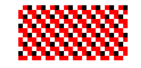
Figure 1: A piece of a PS of a 3-state rule. The states 0, 1 and 2 are represented by white, red and black cells, respectively.

To give an example, Figure 1 displays a piece of the space-time configuration of a 3-state 2-neighbor rule. The spatial and temporal axes are oriented horizontally rightward and downward, respectively, as is common in this field. This PS is generated by any 2-neighbor rule with $3$ states that satisfies $2\underline{0}\mapsto 1$, $1\underline{2}\mapsto 1$, $1\underline{1}\mapsto 1$, $1\underline{0}\mapsto 2$, and $0\underline{1}\mapsto 0$. The initial configuration $012^{\infty}$ re-appears for the first time after $6$ updates, thus in this case $\tau=6$, $\sigma=3$, and the tile (which is, by definition, unique) is

$$\begin{matrix}0&1&2\\ 1&0&1\\ 1&2&0\\ 0&1&1\\ 2&0&1\\ 1&1&0\\ \end{matrix}\quad.$$

Periodic configurations generated by CA have received some attention in the mathematical literature. The groundwork was laid in [23], which extensively studied additive CA, but also devoted some attention to non-additive ones. An important observation is the link between periodicity in CA and state transition diagrams, which we find useful in this paper as well. Successors of [23] include [17, 18, 16, 30, 31, 20]. In [7, 6], the authors take a dynamical systems point of view and explore the density of temporally and spatially periodic (which they call jointly periodic) configurations. Our research is also motivated by [12], where the authors investigate 3-neighbor binary CA and their PS that expand into any environment with positive speed.

Long temporal periods generated by CA have been of particular interest because of their applications to random number generation [29, 9, 27, 26, 24, 10]. In this paper, we focus on this aspect of randomly selected rules, a subject which so far remained unexplored, to our knowledge. For a fixed $n$ and $r$, the natural probability space is $\Omega_{r,n}$, containing all the $n^{n^{r}}$ $r$-neighbor rules, with $\mathbb{P}$ that assigns the uniform probability $\mathbb{P}(\{f\})=1/|\Omega_{r,n}|=1/n^{n^{r}}$ to every $f\in\Omega_{r,n}$. We also fix the spatial period $\sigma$, and define the random variable $X_{\sigma,n}$ by letting $X_{\sigma,n}(f)$ be the longest temporal period with spatial period $\sigma$, for any rule $f\in\Omega_{r,n}$. We are interested in the typical size of $X_{\sigma,n}$ when $r$ and $\sigma$ are fixed and $n$ is large. Our main result covers the case $\sigma\leq r$. The case $\sigma>r$ is much harder, but we expect the same result to hold; see the discussion in Section 4.

Theorem 1.

Fix a number of neighbors $r$ and a spatial period $\sigma\leq r$. Then $\displaystyle\frac{X_{\sigma,n}}{n^{\sigma/2}}$ converges in distribution, as $n\to\infty$, to a nontrivial limit.

Computations with the limiting distribution are a challenge, so we resort to Monte-Carlo simulations in Section 6 to illustrate Theorem 1.

In our companion paper [14], we assume that $r=2$ and show that the limiting probability, as $n\to\infty$, that a random rule has a PS with temporal and spatial periods confined to a finite set $\mathcal{T}\times\Sigma\subset\mathbb{N}\times\mathbb{N}$, is nontrivial and can be computed explicitly. Consequently, we answer another natural question, on the asymptotic size of the shortest temporal period $Y_{\sigma,n}$ of random-rule PS with a spatial period $\sigma$. This random variable converges to a nontrivial distribution ([14], Corollary 3), and is therefore much smaller than $X_{\sigma,n}$, which is on the order $n^{\sigma/2}$, at least for $r=\sigma=2$. It is also interesting to compare the typical value of $X_{\sigma,n}$ to its maximum over all rules [13]. It turns out that even $\max_{f}Y_{\sigma,n}(f)$ is on the order of $n^{\sigma}$ (which, by the pigeonhole principle, is the largest possible).

We now give an outline of the rest of the paper. In Section 2, we construct a directed graph, similar to the one in [14], and its use in analysis of PS is spelled out in Section 3. The proof of Theorem 1 is finally given in Section 5. On the way, we prove the following theorem, which may be of independent interest, in which $C_{n}=C_{\sigma,n}$ is the number of equivalence classes of initial conditions, modulo translations, that are periodic with (minimal) period $\sigma$ and are such that the CA evolution never reduces the spatial period.

Theorem 2.

Assume $\sigma\leq r$. If $\sigma$ is even, then, as $n\to\infty$, $n^{-\sigma}C_{n}$ converges in distribution to $1-\tau$, where $\tau$ is the hitting time of $0$ of the Brownian bridge $\eta(t)$ that starts at $\eta(0)=1/\sqrt{\sigma}$ and ends at $\eta(1)=0$. If $\sigma$ is odd, $n^{-\sigma}C_{n}\to 1$ in probability.

See [2, 1] for related results on random mappings. To prove Theorem 2, we present a sequential construction of the random rule that yields a stochastic difference equation whose solution converges to the Brownian bridge. Once Theorem 2 is established, the remainder of the proof of Theorem 1 is largely an application of existing results on random mappings and random permutations, which we adapt to our purposes in Section 4. In our final Section 6, we discuss extensions of our results, present several simulation results and propose a few open problems for future consideration.

2 The directed graph on equivalence classes of configurations

In this section, we introduce a variant of the configuration digraph [14], a concept introduced in [28]. While conceptually straightforward, this is a very convenient tool to study temporal periods of PS with a fixed spatial period $\sigma\geq 1$. In a sense, it is dual to the label digraph [12, 14], where a temporal period is fixed instead. It will be convenient to interpret periodic configuration with a spatial period $\sigma$, or a divisor of $\sigma$, as evolving on the finite interval $\{0,\ldots,\sigma-1\}$ with periodic boundary conditions, as in [28]. All our finite configurations will be on this interval, with indices taken modulo $\sigma$. We use the standard notation $\mu$ and $\varphi$ for Möbius and Euler totient function.

Definition 2.1.

Fix a spatial period $\sigma\geq 1$ and an $r$-neighbor rule $f$. Let $A=a_{0}\dots a_{\sigma-1}$ and $B=b_{0}\dots b_{\sigma-1}$ be two configurations. We say that $A$ down-extends to $B$ if the rule maps $A$ to $B$ in one update, that is,

$$f(a_{i-r+1},\ldots,a_{i})=b_{i},\quad i=0,\ldots,\sigma-1,$$

and we write $A\searrow B$.

For example, if $f$ is the rule with the PS of Figure 1, and $\sigma=3$, then $012\searrow 101\searrow 120$, etc.

Definition 2.2.

Fix a spatial period $\sigma$ and suppose $\sigma^{\prime}$ is a proper divisor of $\sigma$. A configuration $A=a_{0}\dots a_{\sigma-1}$ is periodic with period $\sigma^{\prime}$ if it can be divided into $\sigma/\sigma^{\prime}>1$ identical words, and $\sigma^{\prime}$ is the smallest such number. If no such $\sigma^{\prime}$ exists, $A$ is aperiodic.

Lemma 2.3.

The number of length-$\sigma$ $n$-state aperiodic configurations is

$$T(\sigma,n)=\sum_{d\bigm{|}\sigma}n^{d}\mu\left(\frac{\sigma}{d}\right)=\begin{cases}n^{\sigma}-n^{\sigma/2}+o(n^{\sigma/2}),&\text{if }\sigma\text{ is even}\\ n^{\sigma}+o(n^{\sigma/2}),&\text{if }\sigma\text{ is odd}\end{cases}.$$

Proof.

See [8]. ∎

Definition 2.4.

Let $\mathbb{Z}_{n}^{\sigma}$ consist of all length-$\sigma$ configurations. A circular shift is a map $\pi:\mathbb{Z}_{n}^{\sigma}\to\mathbb{Z}_{n}^{\sigma}$, satisfying $\pi(a_{0}a_{1}\dots a_{\sigma-1})=a_{\ell}a_{\ell+1}\dots a_{\sigma-1+\ell}$ for some $\ell\in\mathbb{Z}_{+}$ , for all $a_{0}a_{1}\dots a_{\sigma-1}\in\mathbb{Z}_{n}^{\sigma}$ (recall the subscripts are taken modulo of $\sigma$). The order of a circular shift $\pi$ is the smallest $k$ such that $\pi^{k}(A)=A$ for all $A\in\mathbb{Z}_{n}^{\sigma}$, and is denoted by $\text{\rm ord}(\pi)$.

We say that $A$ is equal to $B$ up to circular shift, or in short $A$ is equivalent to $B$, if there is a circular shift $\pi:\mathbb{Z}_{n}^{\sigma}\to\mathbb{Z}_{n}^{\sigma}$ such that $A=\pi(B)$. We record the following observation from [14].

Lemma 2.5.

Let $\pi$ be a circular shift on $\mathbb{Z}_{n}^{\sigma}$ and $A\in\mathbb{Z}_{n}^{\sigma}$ be any aperiodic finite configuration. Then: (1) ord$(\pi)\bigm{|}\sigma$; and (2) if $d\bigm{|}\sigma$, then $|\left\{B\in\mathbb{Z}_{n}^{\sigma}:A=\pi(B)\text{ for some }\pi\text{ with }\text{\rm ord}(\pi)=d\right\}|=\varphi(d)$.

As $A\searrow B$ implies $\pi(A)\searrow\pi(B)$ for any circular shift $\pi$, this relation defined a directed graph on equivalence classes in [14]. We now define a convenient variant, which we call the digraph on equivalence classes (DEC) $G_{\sigma}(f)=(V_{\sigma},E_{\sigma}(f))$, associated with $f$ and $\sigma$. Under the equivalence relation defined above, $\mathbb{Z}_{n}^{\sigma}$ is partitioned into equivalence classes, which inherit periodicy or aperiodicity from their representatives. Note that the cardinality of an aperiodic equivalence class is $\sigma$, while the cardinality of a periodic equivalence class is a proper divisor of $\sigma$. We regard each aperiodic equivalence class as a single vertex, called aperiodic vertex, of the DEC; thus there are $\frac{T(\sigma,n)}{\sigma}$ aperiodic vertices.

Next, we combine periodic classes together to form vertices called periodic vertices, so that, with one possible exception, each vertex contains $\sigma$ configurations. This can be achieved for a large enough $n$ (certainly for $n\geq\sigma^{2}$) as follows. For each proper division $\sigma^{\prime}>1$ of $\sigma$, divide all configurations with period $\sigma^{\prime}$ into sets, which all have cardinality $\sigma$, except for possibly one set; fill that last set with the necessary number of period-1 configurations to make its cardinality $\sigma$. Each of these sets represents a different periodic vertex. At the end, we have $\iota=n^{\sigma}-T(\sigma,n)-\sigma\lfloor\frac{n^{\sigma}-T(\sigma,n)}{\sigma}\rfloor<\sigma$ leftover period-1 configurations, which we combine into the exceptional initial periodic vertex, denoted by $v_{0}$. We let $V_{a}$ and $V_{p}$ be the sets of aperiodic and periodic vertices, so that the vertex set is $V_{\sigma}=V_{a}\cup V_{p}\cup\{v_{0}\}$.

Having completed the definition of the vertex set of DEC, we now specify its set $E_{\sigma}(f)$ of directed edges. An arc $\overrightarrow{uv}\in E_{\sigma}(f)$ if and only if: 1. $u\in V_{a}$, $v\in V_{\sigma}$; and 2. there exist $A\in u$ and $B\in v$ such that $A\searrow B$.

An example of DEC with $\sigma=2$ of a $5$-state rule is given in Figure 2. In this example, $V_{p}=\left\{\left\{00,11\right\},\left\{22,33\right\}\right\}$, $v_{0}=\left\{44\right\}$ and other vertices are all in $V_{a}$. We do not completely specify the rule that generate this DEC, as different CA rules (even a with different range $r$) may induce the same DEC.

Figure 2: DEC of a $2$-neighbor, $5$-state rule.

The set of all DEC’s generated by $r$-neighbor $n$-state rules is denoted by $\mathcal{G}_{\sigma}=\mathcal{G}_{\sigma,r,n}$. Choosing $f$ at random, we obtain a random DEC denoted by $G_{\sigma}=(V_{\sigma},E_{\sigma})\in\mathcal{G}_{\sigma}$. We now give the resulting distribution of $G_{\sigma}$.

Lemma 2.6.

For any $u\in V_{a}$ and $v\in V_{\sigma}$

$$\mathbb{P}(\overrightarrow{uv}\in E_{\sigma})=\begin{cases}\frac{\sigma}{n^{\sigma}},&\text{if }v\neq v_{0}\\ \frac{\iota}{n^{\sigma}},&\text{if }v=v_{0}\\ \end{cases}.$$

Proof.

For any configurations $A\in u$ and $B\in v$, $\mathbb{P}(A\searrow B)=1/n^{\sigma}$. Then $\mathbb{P}(\overrightarrow{uv}\in E_{\sigma})=|v|\mathbb{P}(A\searrow B)$, giving the desired result. ∎

3 The connection between DEC and PS

In a DEC, we call a vertex to be a cemetery vertex if it is either a periodic vertex or there is a directed path from it to a periodic vertex (which, we repeat, is a set of configurations with spatial periods less than $\sigma$). Otherwise, a vertex is said to be non-cemetery. For example, in Figure 2, the vertices $\{00,11\}$, $\{22,33\}$ and $\{44\}$ are cemetery as they are periodic; $\{03,30\}$, $\{04,40\}$, $\{12,21\}$, $\{14,41\}$ and $\{13,31\}$ are also cemetery as there exists a directed path from each of them to a periodic vertex; other five vertices are non-cemetery. The reason that we declare a vertex $C\ni A$ of length $\sigma$ to be cemetery is that when the CA updates to configuration $A$, the spatial period is reduced and the dynamics cannot produce a PS of spatial period $\sigma$. For example, in the DEC of Figure 2, a PS with $\sigma=2$ cannot contain the configuration $21$, as its appearance leads to $44$, which has spatial period $1$.

It is also important to note that different rules can have the same DEC. In particular, a cycle in a DEC may generate PS with different temporal periods depending on the rule. We illustrate this by the $\sigma=2$ example in Figure 2. First, we locate a directed cycle, say, the one of length 3. Using a configuration from any vertex on the cycle, say $23$, as the initial configuration, run the rule starting with $23$ until $23$ appears again. Now, the temporal period can be either 3 or 6, depending on the rule $f$. Namely, if the rule assignments result in, say, $23\searrow 24\searrow 43\searrow 23$, then $\tau=3$, while if they are $23\searrow 24\searrow 43\searrow 32$, then $\tau=6$. In general, if a cycle in DEC has length $\ell$, then the corresponding temporal period of the PS generated by this cycle may have length $d\ell$, where $d$ is any divisor of $\sigma$.

For an arbitrary $G\in\mathcal{G}_{\sigma}$, define $M(G)$ to be the number of directed cycles in $G$. (For example, $M(G)=2$ for $G$ in Figure 2.) Let $L_{i}(G)$ be the length of the $i$th longest directed cycle $C^{(i)}(G)$ of $G$, with $L_{i}(G)=0$ for $i>M(G)$. Then, for a rule $f$, define $M(f)=M(G_{\sigma}(f))$ and $L_{i}(f)=L_{i}(G_{\sigma}(f))$. Furthermore, if a PS of temporal period $d\ell$ results from a cycle $C$ of length $\ell$ in $G_{\sigma}(f)$, we say that $C$ has expanding number $d$ under $f$, and use the notation $E_{f}(C)=d$. We let $E_{i}(f)=E_{f}(C^{(i)}(G_{\sigma}(f)))$, again defined to be $0$ when $C^{(i)}(G_{\sigma}(f))$ does not exist, i.e., when $i>M(f)$. We state the connection between the longest temporal period and the cycle length in DEC in the following lemma.

Lemma 3.1.

Let $f$ be a CA rule and $G_{\sigma}(f)$ be its DEC of period $\sigma$. Then we have

$$X_{\sigma,n}(f)=\max\left\{L_{i}(f)\cdot E_{i}(f):i=1,2,\ldots\right\}.$$

Moreover, if $C^{(k)}(G_{\sigma}(f))$ is the longest cycle that is $\sigma$-expanded, then

$$X_{\sigma,n}(f)=\max\left\{L_{k}(f)\cdot\sigma,L_{i}(f)\cdot E_{i}(f):i=1,2,\ldots,k-1\right\}.$$

Proof.

The first part is clear from the definition, and the second part follows as $\sigma$ is the largest possible expanding number. ∎

As a consequence of the above lemma, our task is to study the properties of DEC and expanding numbers when a rule is randomly selected. A random DEC is essentially a random mapping, after eliminating cemetery vertices, as we will see. We formulate a lemma on expanding numbers next.

Lemma 3.2.

Let $G\in\mathcal{G}_{\sigma}$ be a fixed DEC, and $\sigma\leq r$. Select a rule $f$ at random. Then, conditioned on the event $\left\{G_{\sigma}(f)=G\right\}$, the random variables $E_{i}(f)$, $i=1,\dots,M(G)$, are independent. Also

$$\mathbb{P}\left(E_{i}(f)=d\biggm{|}G_{\sigma}(f)=G\right)=\frac{\varphi(d)}{\sigma},$$

for $i=1,\dots,M(G)$ and $d\bigm{|}\sigma$.

Proof.

Let a cycle $C^{(i)}(G)$ be $v_{1}\to v_{2}\to\dots\to v_{k}\to v_{1}$. Let $A_{j}$’s be configurations of length $\sigma$ such that $A_{j}\in v_{j}$, $j=1,\dots,k$. Then there are circular shifts, $\pi_{j}$’s, $j=1,\dots,k$, such that $A_{1}\searrow\pi_{2}(A_{2})\searrow\dots\searrow\pi_{k}(A_{k})\searrow\pi_{1}(A_{1})$, under rule $f$. Now, $E_{i}(f)=d$ if and only if ord$(\pi_{1})=d$, which is independent from other cycles as $\sigma\leq r$ and has the desired probability by Lemma 2.5. ∎

In summary, we may study the probabilistic behavior of $X_{\sigma,n}$ by moving from the sample space $\Omega_{r,n}$ to $\mathcal{G}_{\sigma}\times\Xi_{\sigma}^{\infty}$, where $\Xi_{\sigma}=\{d\in\mathbb{N}:d\bigm{|}\sigma\}$. The marginal probability distributions on components are independent from each other. The distribution on $\mathcal{G}_{\sigma}$ is given in Lemma 2.6, while the distribution on each component of $\Xi_{\sigma}^{\infty}$ is given by Lemma 3.2: $\mathbb{P}\left(\{w\}\right)=\frac{\varphi(w)}{\sigma}$, for $w\in\Xi_{\sigma}$. If the random variables $T_{i}:\Xi_{\sigma}\to\Xi_{\sigma}$ are defined to be identities, then the distribution of $X_{\sigma,n}$ is given by

$$\max\left\{L_{i}\left(G_{\sigma}\right)\cdot T_{i}(w):i=1,2,\dots\right\}=:\max\left\{L_{i}\cdot T_{i}:i=1,2,\dots\right\}.$$

Let $K_{\sigma}=\min\{i:T_{i}=\sigma\}$ be a random variable on $\Xi_{\sigma}^{\infty}$, representing the smallest index of $T_{i}$’s that is equal to $\sigma$. Then $\mathbb{P}\left(K_{\sigma}=k\right)=\left(1-\frac{\varphi(\sigma)}{\sigma}\right)^{k-1}\left(\frac{\varphi(\sigma)}{\sigma}\right)$ for $k\geq 1$, i.e., $K_{\sigma}$ is $\text{Geometric}\left(\frac{\varphi(\sigma)}{\sigma}\right)$. Then we may write

$$X_{\sigma,n}=\max\left\{L_{i}\cdot T_{i}^{\prime},L_{K_{\sigma}}\sigma,i=1,2,\dots,K_{\sigma}-1\right\},$$

where $\mathbb{P}\left(T_{i}^{\prime}=d\right)=\mathbb{P}\left(T_{i}=d\bigm{|}T_{i}\neq\sigma\right)=\frac{\varphi(d)}{\sigma-\varphi(\sigma)}$, for $d\bigm{|}\sigma$ and $d\neq\sigma$.

4 Random mappings

In this section, we discuss a result about the cycle structure of random mapping, indicating that the joint distribution of the longest $k$ cycles converges after a proper scaling.

We will consider the function space $\mathcal{R}_{N}=\{g:\mathbb{Z}_{N}\to\mathbb{Z}_{N}\}$ containing all functions from $\mathbb{Z}_{N}$ into itself. Clearly $|\mathcal{R}_{N}|=N^{N}$. A finite sequence $x_{0},\dots,x_{\ell-1}\in\mathbb{Z}_{N}$ is a cycle of length $\ell$ if $g(x_{0})=x_{1},g(x_{1})=x_{2},\dots,g(x_{\ell-2})=x_{\ell-1}$ and $g(x_{\ell-1})=x_{0}$. We call $g$ a random mapping if $g$ is randomly and uniformly selected from $\mathcal{R}_{N}$. Let $P_{N}^{(k)}$ be the random variable representing the $k$th longest cycle length of a random mapping from $\mathcal{R}_{N}$. More extensively studied function space is $\mathcal{S}_{N}=\{g:\mathbb{Z}_{N}\to\mathbb{Z}_{N}:g\text{ is bijective}\}$ containing all permutations of $\mathbb{Z}_{N}$. Clearly, $|\mathcal{S}_{N}|=N!$ and a cycle can be defined in the same way. We call $g$ a random permutation if $g$ is randomly and uniformly selected from $\mathcal{S}_{N}$ and we use $Q_{N}^{(k)}$ to denote the random variable representing the $k$th longest cycle length of a random permutation from $\mathcal{S}_{N}$. The probabilistic properties of $P_{N}^{(k)}$ and $Q_{N}^{(k)}$ have been investigated in a number of papers, including [4, 11, 3, 15].

What is relevant to us is the distribution of $\left(P_{N}^{(1)},P_{N}^{(2)},\dots,P_{N}^{(k)}\right)$ as $N\to\infty$, for which we are not aware of a direct reference. We can, however, use the fact that for a random mapping, conditioning on the set of elements that belong to cycles generates a random permutation. To begin, we let $M_{N}$ be the number of elements from $\mathbb{Z}_{N}$ that belong to cycles of a random mapping from $\mathcal{R}_{N}$. The following well-known result provides the distribution of $M_{N}$, see [4] or [5].

Lemma 4.1.

We have

$$\mathbb{P}\left(M_{N}=s\right)=\frac{s}{N}\prod_{j=1}^{s-1}\left(1-\frac{j}{N}\right),\quad s=1,\dots,N.$$

The next result is adapted from Corollary 5.11 in [3].

Proposition 4.2.

As $N\to\infty$,

$$\frac{1}{N}\left(Q_{N}^{(1)},Q_{N}^{(2)},\dots\right)\to\left(Q^{(1)},Q^{(2)},\dots\right),\text{ in distribution},$$

in $\Delta=\{(x_{1},x_{2},\dots)\subset(0,1)^{\infty}:\sum_{i}x_{i}=1\}$. Here, for each $k$, $\left(Q^{(1)},Q^{(2)},\dots,Q^{(k)}\right)$ has density

$$q^{(k)}(x_{1},\dots,x_{k})=\frac{1}{x_{1}x_{2}\cdots x_{k}}\left(1+\sum_{j=1}^{\infty}\frac{(-1)^{j}}{j!}\int_{I_{j}(x)}\frac{dy_{1}\cdots dy_{j}}{y_{1}\dots y_{j}}\right),$$

on $\Delta$, where $I_{j}(x)$ is the set of $(y_{1},\dots,y_{j})$ that satisfy

$$\min\{y_{1},\dots,y_{j}\}>x^{-1}\text{ and }y_{1}+\dots+y_{j}<1$$

and

$$x=\frac{1-x_{1}-\dots-x_{k}}{x_{k}}.$$

Lemma 4.3.

For a fixed $N$, let

$$h_{N}(x)=\frac{s}{\sqrt{N}}\prod_{j=1}^{s-1}\left(1-\frac{j}{N}\right),$$

for $x\in\left(\frac{s-1}{\sqrt{N}},\frac{s}{\sqrt{N}}\right]$ and $s=1,2,\dots$. Then $h_{N}(x)\leq 4\max\left(x,1\right)\exp\left(-x^{2}/2\right)$ for all $x>0$, which is integrable on $(0,\infty)$. Also, $h_{N}(x)\to x\exp\left(-x^{2}/2\right)$, as $N\to\infty$, for all $x\in(0,\infty)$.

Proof.

Since $h_{N}(x)=0$ for $x>\sqrt{N}$, it suffices to show the inequality for $x\leq\sqrt{N}$, i.e., $s\leq N$. Since $1-\frac{j}{N}<\exp\left(-\frac{j}{N}\right)$ , it follows that $\prod_{j=1}^{s-1}\left(1-\frac{j}{N}\right)<\exp\left(-\frac{s^{2}}{2N}\right)\exp\left(\frac{s}{2N}\right)<2\exp\left(-\frac{s^{2}}{2N}\right)$, for $s\leq N$. So, if $x\in\left(\frac{s-1}{\sqrt{N}},\frac{s}{\sqrt{N}}\right]$, then

$$h_{N}(x)\leq 2\frac{s}{\sqrt{N}}\exp\left(-\frac{x^{2}}{2}\right).$$

When $s=1$, $s/\sqrt{N}\leq 2$, while for $s\geq 2$, $s/\sqrt{N}\leq 2(s-1)/\sqrt{N}\leq 2x$, proving the inequality. To prove convergence, observe that

$$h_{N}(x) =\frac{\lceil\sqrt{N}x\rceil}{\sqrt{N}}\prod_{j=1}^{\lceil\sqrt{N}x\rceil-1}\left(1-\frac{j}{N}\right)$$

$$=\frac{\lceil\sqrt{N}x\rceil}{\sqrt{N}}\prod_{j=1}^{\lceil\sqrt{N}x\rceil-1}\exp\left\{-\frac{j}{N}+\mathcal{O}\left(\frac{j^{2}}{N^{2}}\right)\right\}$$

$$=\frac{\lceil\sqrt{N}x\rceil}{\sqrt{N}}\exp\left[-\frac{\lceil\sqrt{N}x\rceil\left(\lceil\sqrt{N}x\rceil-1\right)}{2N}+\mathcal{O}\left(\frac{1}{\sqrt{N}}\right)\right]$$

$$\to x\exp\left({-x^{2}}/{2}\right),$$

as $N\to\infty$.∎

Theorem 3.

Let $P_{N}^{(k)}$ be the $k$th longest cycle length in a random mapping from $\mathcal{R}_{N}$. Then

$$N^{-1/2}\left(P_{N}^{(1)},P_{N}^{(2)},\dots,P_{N}^{(k)}\right)$$

converges to a nontrivial joint distribution, as $N\to\infty$.

Proof.

Conditioning on the event that a set $S\subset\mathbb{Z}_{N}$ is exactly the set of elements of $\mathbb{Z}_{N}$ that belong to cycles, the random mapping is a random permutation of $S$. It follows that for any bounded continuous function $\phi:\mathbb{R}^{k}\to\mathbb{R}$,

$$\mathbb{E}\left[\phi\left(\frac{P_{N}^{(1)}}{\sqrt{N}},\dots,\frac{P_{N}^{(k)}}{\sqrt{N}}\right)\right] =\sum_{s=1}^{N}\mathbb{E}\left[\phi\left(\frac{P_{N}^{(1)}}{\sqrt{N}},\dots,\frac{P_{N}^{(k)}}{\sqrt{N}}\right)\biggm{|}M_{N}=s\right]\mathbb{P}\left(M_{N}=s\right)$$

$$=\sum_{s=1}^{N}\mathbb{E}\left[\phi\left(\frac{Q_{s}^{(1)}}{\sqrt{N}},\dots,\frac{Q_{s}^{(k)}}{\sqrt{N}}\right)\right]\frac{s}{N}\prod_{j=1}^{s-1}\left(1-\frac{j}{N}\right)$$

$$=\sum_{s=1}^{N}\mathbb{E}\left[\phi\left(\frac{Q_{s}^{(1)}}{s}\frac{s}{\sqrt{N}},\dots,\frac{Q_{s}^{(k)}}{s}\frac{s}{\sqrt{N}}\right)\right]\frac{s}{N}\prod_{j=1}^{s-1}\left(1-\frac{j}{N}\right).$$

Define $\widetilde{h}_{N}:\mathbb{R}\to\mathbb{R}$

$$\widetilde{h}_{N}(x)=\mathbb{E}\left[\phi\left(\frac{Q_{s}^{(1)}}{s}\frac{s}{\sqrt{N}},\dots,\frac{Q_{s}^{(k)}}{s}\frac{s}{\sqrt{N}}\right)\right]\frac{s}{\sqrt{N}}\prod_{j=1}^{s-1}\left(1-\frac{j}{N}\right),$$

for $x\in\left(\frac{s-1}{\sqrt{N}},\frac{s}{\sqrt{N}}\right]$, $s=1,2,\dots$ By Lemma 4.3 and Proposition 4.2, $\widetilde{h}_{N}$ is bounded by an integrable function and, for every fixed $x\geq 0$,

$$\lim_{n\to\infty}\widetilde{h}_{N}(x) =\lim_{N\to\infty}\mathbb{E}\left[\phi\left(\frac{Q_{\lceil\sqrt{N}x\rceil}^{(1)}}{{\lceil\sqrt{N}x\rceil}}\frac{{\lceil\sqrt{N}x\rceil}}{\sqrt{N}},\dots,\frac{Q_{\lceil\sqrt{N}x\rceil}^{(k)}}{{\lceil\sqrt{N}x\rceil}}\frac{{\lceil\sqrt{N}x\rceil}}{\sqrt{N}}\right)\right]x\exp\left(-\frac{x^{2}}{2}\right)$$

$$=\mathbb{E}\left[\phi\left(Q^{(1)}x,\dots,Q^{(k)}x\right)\right]x\exp\left(-\frac{x^{2}}{2}\right).$$

Then,

$$\lim_{N\to\infty}\mathbb{E}\left[\phi\left(\frac{P_{N}^{(1)}}{\sqrt{N}},\dots,\frac{P_{N}^{(k)}}{\sqrt{N}}\right)\right]$$

$$=\lim_{N\to\infty}\int_{0}^{\infty}\widetilde{h}_{N}(x)dx$$

$$=\int_{0}^{\infty}\mathbb{E}\left[\phi\left(Q^{(1)}x,\dots,Q^{(k)}x\right)\right]x\exp\left(-\frac{x^{2}}{2}\right)dx,$$

by dominated convergence theorem. ∎

As a consequence, we obtain the following convergence in distribution.

Lemma 4.4.

Let $T_{j}^{\prime}$’s, for $j=1,2,\dots$, be i.i.d. with

$$\mathbb{P}\left(T_{j}^{\prime}=d\right)=\frac{\varphi(d)}{\sigma-\varphi(\sigma)},$$

for all divisors $d\neq\sigma$ of $\sigma$, and independent of the random mapping. Let

$$D_{N}^{(k)}=\max\left\{P_{N}^{(k)}\cdot\sigma,P_{N}^{(j)}\cdot T_{j}^{\prime}:j=1,2,\dots,k-1\right\}.$$

Then $N^{-1/2}D_{N}^{(k)}$ converges to a nontrivial distribution, for any $k$ and $\sigma$.

Proof.

Note that $T_{j}^{\prime}$’s do not depend on $N$. So the vector $N^{-1/2}\left(P_{N}^{(1)}T_{1}^{\prime},\dots,P_{N}^{(k-1)}T_{k-1}^{\prime},P_{N}^{(k)}\sigma\right)$ converges in distribution as $N\to\infty$. The conclusion follows by continuity. ∎

In the sequel, we denote by $D^{(k)}$ a generic random variable with the limiting distribution of $N^{-1/2}D_{N}^{(k)}$.

5 The main results

5.1 The case $\sigma=1$

In this case, a DEC does not have cemetery vertices thus our problem simply reduces to a random mapping problem. To be precise,

(2) $$\frac{X_{1,n}}{n^{1/2}}=\frac{L_{1}}{n^{1/2}}=_{d}\frac{P_{n}^{(1)}}{n^{1/2}},$$

which converges in distribution by Theorem 3. The first equality in (2) holds because a cycle in a DEC cannot be expanded when $\sigma=1$ and the second equality in (2) is true because there are no cemetery states for $\sigma=1$.

For a general $\sigma$, the problem may be handled similarly to the case of $\sigma=1$ only after eliminating the cemetery vertices. As a consequence, we must determine the behavior of $C_{n}=C_{\sigma,n}$ from Section 1, which we may reinterpret as the random variable representing the number of non-cemetery vertices in a DEC of spatial period $\sigma$. The strategy is as follows: construct the random DEC via a sequential algorithm that naturally provides a system of stochastic difference equations for the number of non-cemetery classes with $C_{n}$ related to a hitting time; then show that the solution of the stochastic difference equations, appropriately scaled, converges to a diffusion, giving the asymptotic behavior of $C_{n}$.

5.2 Construction of a random DEC and the difference equations

$C_{A}\leftarrow V_{p}\cup\{v_{0}\}$ or $V_{p}$, if $v_{0}$ does not exist

  // Active cemetery vertices

$C_{P}\leftarrow\emptyset$

  // Passive cemetery vertices

$C_{N}\leftarrow V_{a}$

  // Non-cemetery vertices

$E\leftarrow\emptyset$

  // Set of arcs

$k\leftarrow 0$

$Y_{0}\leftarrow|C_{N}|$

$Z_{0}\leftarrow|C_{A}|$

if $v_{0}\in C_{A}$ then // If $v_{0}$ exists

       $C_{A}\leftarrow C_{A}\setminus\{v_{0}\}$

       $C_{P}\leftarrow C_{P}\cup\{v_{0}\}$

        // Make it passive

       Let $\beta_{0}\sim\text{\rm Binomial}\left(Y_{0},\frac{\iota}{n^{\sigma}}\right)$

       Pick random $v_{1},\dots,v_{\beta_{0}}$ in $C_{N}$

        // Select non-cemetery vertices that map to $v_{0}$

       for $j=1,\dots,\beta_{0}$ do

             $E\leftarrow E\cup\{\overrightarrow{v_{j}v_{0}}\}$

              // Add the arcs to the set of arcs

             $C_{A}\leftarrow C_{A}\cup\{v_{j}\}$

              // Make the vertices active cemetery

             $C_{N}\leftarrow C_{N}\setminus\{v_{j}\}$

            

       end for

      $Y_{0}\leftarrow|C_{N}|$

        // Update the number of temporary non-cemetery vertices

       $Z_{0}\leftarrow|C_{A}|$

        // Update the number of active cemetery vertices

       $k\leftarrow 1$

end if

while $|C_{A}|>0$ do // When $C_{A}=\emptyset$, the non-cemetery vertices are determined

       Pick a random $v\in C_{A}$

        // Pick a random active cemetery vertex $v$

       $C_{A}\leftarrow C_{A}\setminus\{v\}$

       $C_{P}\leftarrow C_{P}\cup\{v\}$

        // Make $v$ passive

       Let $\beta_{k}\sim\text{\rm Binomial}\left(Y_{k},\frac{1}{Y_{k}+Z_{k}}\right)$

       Pick random $v_{1},\dots,v_{\beta_{k}}$ in $C_{N}$

        // Select non-cemetery vertices that map to $v$

       for $j=1,\dots,\beta_{k}$ do

             $E\leftarrow E\cup\{\overrightarrow{v_{j}v}\}$

              // Add the arcs to the set of arcs

             $C_{A}\leftarrow C_{A}\cup\{v_{j}\}$

              // Make the vertices active cemetery

             $C_{N}\leftarrow C_{N}\setminus\{v_{j}\}$

            

       end for

      $Y_{k}\leftarrow|C_{N}|$

        // Update the number of non-cemetery vertices

       $Z_{k}\leftarrow|C_{A}|$

        // Update the number of active cemetery vertices

       $k\leftarrow k+1$

      

end while

for $v\in C_{N}$ do // Assign arcs among non-cemetery vertices.

       Pick a $u$ uniformly from $C_{N}$

       $E=E\cup\{\overrightarrow{vu}\}$

      

end for

Algorithm 1 Construction of a random DEC

Recall the notation from Section 2 and Lemma 2.6. Algorithm 1 formally describes a way of generating a random DEC that sequentially adds cemetery vertices until all are gathered. The procedure specifies the evolution of the set of cemetery vertices, which are separated into active and passive ones, initially all active. In the $k$th step ($k=0,1,\dots$), we pick an active cemetery vertex $v$, making it passive. We also select $\beta_{k}$ non-cemetery vertices that map to $v$, where $\beta_{k}\sim\text{\rm Binomial}\left(Y_{k},\frac{1}{Y_{k}+Z_{k}}\right)$. (If $k=0$ and $v_{0}$ exists, the initial pick is $v_{0}$ and the probability changes accordingly.) This distribution is justified by Lemma 2.6, i.e., all non-cemetery vertex share the same probability of mapping into a vertex that is not passive cemetery. We make those $\beta_{k}$ vertices active cemetery, because each one of them has the ability to “absorb” non-cemetery vertices (thus is active), while itself maps into a periodic class of a lower period along a directed path (thus is cemetery). The above procedure determines all cemetery classes in the while loop. In the final for loop, we assign a unique target uniformly for each non-cemetery vertex. Note that $Y_{k}$ and $Z_{k}$ are the numbers of non-cemetery and active cemetery vertices at the end of $k$th iteration of the while loop.

Now, letting $\Delta Y_{k}=Y_{k+1}-Y_{k}$, and $\Delta Z_{k}=Z_{k+1}-Z_{k}$, we obtain the stochastic difference equation for $k$ such that $Z_{k}\geq 0$,

(3) $$\begin{cases}\Delta Y_{k}=-1-\Delta Z_{k}=-\beta_{k}\\ \Delta Z_{k}=\beta_{k}-1=\frac{Y_{k}}{Y_{k}+Z_{k}}-1+\Delta B_{k}\sqrt{\frac{Y_{k}}{Y_{k}+Z_{k}}\left(1-\frac{1}{Y_{k}+Z_{k}}\right)}\end{cases},$$

where $\beta_{k}$’s are independent and

$$\beta_{k}\sim\text{\rm Binomial}\left(Y_{k},\frac{1}{Y_{k}+Z_{k}}\right),$$

for $k=1,2,\dots$, thus

$$\Delta B_{k}=\frac{\beta_{k}-Y_{k}/(Y_{k}+Z_{k})}{\sqrt{\frac{Y_{k}}{Y_{k}+Z_{k}}\left(1-\frac{1}{Y_{k}+Z_{k}}\right)}}.$$

For the initial condition, we have

$$Y_{0}=\begin{cases}-B_{0}+\frac{T(\sigma,n)}{\sigma},&\text{if }\iota=0\\ -B_{1}+\frac{T(\sigma,n)}{\sigma},&\text{if }\iota\neq 0\\ \end{cases},$$

and

$$Z_{0}=\begin{cases}B_{0}-1+\lfloor\frac{n^{\sigma}-T(\sigma,n)}{\sigma}\rfloor,&\text{if }\iota=0\\ B_{1}-1+\lfloor\frac{n^{\sigma}-T(\sigma,n)}{\sigma}\rfloor,&\text{if }\iota\neq 0\\ \end{cases},$$

where $B_{0}\sim\text{\rm Binomial}\left(\frac{T(\sigma,n)}{\sigma},\frac{\sigma}{n^{\sigma}}\right)$ and $B_{\text{1}}\sim\text{\rm Binomial}\left(\frac{T(\sigma,n)}{\sigma},\frac{\iota}{n^{\sigma}}\right)$. To define the processes for all $k=0,1,\dots,N-1$, we stop $Y_{k}$ and $Z_{k}$ once $Z_{k}$ hits zero.

5.3 Convergence to a diffusion

Let $N=|V_{\sigma}|=n^{\sigma}/\sigma+\mathcal{O}(n^{\sigma/2})$ be the total number of vertices. We scale $Y_{k}$ and $Z_{k}$ by dividing by $N$ and $\sqrt{N}$, respectively. To be more precise, consider the 2-dimensional process $\xi_{k,N}=\left(\xi_{k,N}^{(1)},\xi_{k,N}^{(2)}\right)$, for $k=0,\dots,N-1$, where $\xi_{k,N}^{(1)}=Y_{k}/N$ is the scaled number of non-cemetery states and $\xi_{k,N}^{(2)}=Z_{k}/\sqrt{N}$ is the scaled number of active cemetery states. For a fixed $\xi_{k,N}$, let $\tau=\tau\left(\xi_{k,N}\right)=\inf\{k/N:\xi_{k,N}^{(2)}\leq 0\}$ be the hitting time of zero for the second coordinate. We are thus interested in this question: when the number of active cemetery vertices is zero, what is the limiting distribution of proportion of non-cemetery vertices? In other words, what is $\lim\mathbb{P}\left(\xi_{\tau}^{(1)}\leq x\right)$, for $x\in(0,1)$, as $N\to\infty$? We will prove the following result, which is a restatement of Theorem 2.

Theorem 4.

As $N\to\infty$, $\xi_{\tau}^{(1)}\to 1-\tau(\eta)$ in distribution, where $\tau(\eta)=\inf\{t:\eta(t)=0\}$ and $\eta(t)$ satisfies

$$\eta(t)=p(\sigma)-\int_{0}^{t}\frac{\eta(s)}{1-s}ds-B_{t},$$

where $p(\sigma)=1/\sqrt{\sigma}$ if $\sigma$ is even and $p(\sigma)=0$, otherwise. In particular, when $\sigma$ is even, $\xi_{\tau}^{(1)}$ converges to a non-trivial limiting distribution, while when $\sigma$ is odd, $\xi_{\tau}^{(1)}\to 1$ in probability.

Our strategy in proving Theorem 4 is to verify the conditions in [22] for a solution of a stochastic difference equation to converge to a diffusion. However, trying to prove this directly for $\xi_{k,N}$ runs into uniform continuity and boundedness problems, so we need an intermediate process $\widetilde{\xi}_{k,N}$. For a fixed $N$, we define the stochastic difference equations of $\widetilde{\xi}_{k,N}=\left(\widetilde{\xi}_{k,N}^{(1)},\widetilde{\xi}_{k,N}^{(2)}\right)$ by giving $\Delta\widetilde{\xi}_{k,N}^{(i)}=\widetilde{\xi}_{k+1,N}^{(i)}-\widetilde{\xi}_{k,N}^{(i)}$, $i=1,2$, as follows

(4) $$\begin{cases}\Delta\widetilde{\xi}_{k,N}^{(1)}=-\frac{1}{N}-\Delta\widetilde{\xi}_{k,N}^{(2)}\,\frac{1}{\sqrt{N}}\\ \Delta\widetilde{\xi}_{k,N}^{(2)}=-\frac{1}{N}\widetilde{\Psi}+\frac{1}{\sqrt{N}}\Delta\widetilde{b}\,\widetilde{\Upsilon}\end{cases}.$$

The quantities $\widetilde{\Psi}$, $\widetilde{\Upsilon}$, and $\Delta\widetilde{b}$ depend on additional parameters $\delta\geq 0$ and $M\geq 0$. Define

(5) $$g(x)=\max(x,\delta)\text{ and }h(x)=\min(\max(x,-M),M).$$

Then

$$\widetilde{\Psi}=\frac{h\left(\widetilde{\xi}_{k,N}^{(2)}\right)}{g\left(\widetilde{\xi}_{k,N}^{(1)}\right)+h\left(\widetilde{\xi}_{k,N}^{(2)}\right)/\sqrt{N}},$$

$$\widetilde{\Upsilon}=\sqrt{\widetilde{\Phi}\left(1-\frac{1}{\lfloor Ng\left(\widetilde{\xi}_{k,N}^{(1)}\right)\rfloor+\sqrt{N}h\left(\widetilde{\xi}_{k,N}^{(2)}\right)}\right)},$$

$$\Delta\widetilde{b}=\frac{\widetilde{\beta}_{k}-\widetilde{\Phi}}{\widetilde{\Upsilon}},$$

$$\widetilde{\beta}_{k}\sim\text{\rm Binomial}\left(\lfloor Ng\left(\widetilde{\xi}^{(1)}_{k,N}\right)\rfloor,\frac{1}{\lfloor Ng\left(\widetilde{\xi}^{(1)}_{k,N}\right)\rfloor+\sqrt{N}h\left(\widetilde{\xi}^{(2)}_{k,N}\right)}\right),$$

$$\widetilde{\Phi}=\frac{\lfloor Ng\left(\widetilde{\xi}_{k,N}^{(1)}\right)\rfloor}{\lfloor Ng\left(\widetilde{\xi}_{k,N}^{(1)}\right)\rfloor+\sqrt{N}h\left(\widetilde{\xi}_{k,N}^{(2)}\right)}=\mathbb{E}\widetilde{\beta}_{k}.$$

We view the $\widetilde{\Psi}$, $\widetilde{\Upsilon}$, and $\widetilde{\Phi}$ (and their relatives defined later) alternatively as the expressions in $\widetilde{\xi}_{k,N}$ or functions from $\mathbb{R}^{2}$ to $\mathbb{R}$, which use $\widetilde{\xi}_{k,N}$ as values of their independent arguments. When $N>(M/\delta)^{2}$, the denominators in the above expressions are positive, and thus the process is automatically defined for $k=1,\dots,N-1$. When $\delta=0$ and $M=\infty$, the difference equation (4) is exactly the difference equation for $\left(\xi^{(1)}_{k,N},\xi^{(2)}_{k,N}\right)$, when $\xi^{(2)}_{k,N}\geq 0$. We assume $\delta>0$ (but small) and $M<\infty$ (but large) for the rest of this section. The initial conditions for $\widetilde{\xi}_{k,N}$ and ${\xi}_{k,N}$ agree: $\widetilde{\xi}_{0,N}=\xi_{0,N}$. We now record some immediate consequences of the above definitions.

Lemma 5.1.

When $N>(2M/\delta)^{2}$, the following statements hold:

1. For all $k$, $0<\widetilde{\Phi}<3$.

2. For all $k$, $0<\widetilde{\Upsilon}<2$.

3. For all $k$, $|\widetilde{\Psi}|\leq 2M/\delta$.

4. For all $\ell,k\geq 0$,

   $$\mathbb{E}\left|\Delta\widetilde{b}_{k}\widetilde{\Upsilon}\right|^{\ell}\leq D_{\ell},$$

   where $D_{\ell}$ is a constant depending only on $\ell$.

Proof.

Parts 1–3 are clear. For part 4, observe that $\mathbb{E}\left(\Delta\widetilde{b}_{k}\widetilde{\Upsilon}\right)^{\ell}$ is the centered moment of a $\text{\rm Binomial}(x,p)$ random variable with $xp<3$. Then the desired bound follows from Theorem 2.2 in [21] for even $\ell$ and from Cauchy-Schwarz for odd $\ell$. ∎

We have now arrived at the key result on the way to proving Theorems 1 and 2. As usual, the process $\widetilde{\xi}_{t}$ is the piecewise linear process on $[0,1]$, with values $\widetilde{\xi}_{k,N}$ at $k/N$. Furthermore, we define $\widetilde{\eta}_{t}=\left(\widetilde{\eta}_{t}^{(1)},\widetilde{\eta}_{t}^{(2)}\right)$ to be

(6) $$\begin{cases}\widetilde{\eta}_{t}^{(1)}=1-t\\ \widetilde{\eta}_{t}^{(2)}=\displaystyle p(\sigma)-\int_{0}^{t}\frac{h\left(\widetilde{\eta}_{s}^{(2)}\right)}{g(1-s)}ds-B_{t}\end{cases},$$

for $t\in[0,1]$, where $p(\sigma)=1/\sqrt{\sigma}$ if $\sigma$ is even and $p(\sigma)=0$, otherwise.

Lemma 5.2.

As $N\to\infty$, $\widetilde{\xi}_{t}\to\widetilde{\eta}_{t}$ in distribution, in $\mathcal{C}([0,1],\mathbb{R}^{2})$.

Proof.

We write

$$\mathbb{E}\left[\Delta\widetilde{\xi}_{k,N}\biggm{|}\mathcal{F}_{k}\right]=e_{N}\left(\widetilde{\xi}_{k,N}\right)\Delta t_{k}^{N},$$

where $\mathcal{F}_{k}$ is the $\sigma$-algebra generated by $\widetilde{\xi}_{0,N},\ldots,\widetilde{\xi}_{k,N}$, $e_{N}\left(\widetilde{\xi}_{k,N}\right)=\begin{bmatrix}-1+\frac{\widetilde{\Psi}}{\sqrt{N}}\\ -\widetilde{\Psi}\end{bmatrix}$ and $\Delta t_{k}^{N}=1/N$. Moreover,

$$\text{\rm Cov}\left[\Delta\widetilde{\xi}_{k,N}\biggm{|}\mathcal{F}_{k}\right]=s_{N}\left(\widetilde{\xi}_{k,N}\right)s_{N}\left(\widetilde{\xi}_{k,N}\right)^{T}\Delta t_{k}^{N},$$

where $s_{N}\left(\widetilde{\xi}_{k,N}\right)=\begin{bmatrix}\frac{\widetilde{\Upsilon}}{\sqrt{N}}\\ -\widetilde{\Upsilon}\end{bmatrix}$ and $s_{N}\left(\widetilde{\xi}_{k,N}\right)^{T}$ is its transpose. Now, define

$$e\left(\widetilde{\xi}_{k,N}\right)=\begin{bmatrix}-1\\ -\overline{\Psi}\end{bmatrix},$$

and

$$s\left(\widetilde{\xi}_{k,N}\right)=\begin{bmatrix}0\\ -1\end{bmatrix},$$

where

$$\overline{\Psi}=\frac{h\left(\widetilde{\xi}_{k,N}^{(2)}\right)}{g\left(\widetilde{\xi}_{k,N}^{(1)}\right)}.$$

In the following steps, we suppress the value $\widetilde{\xi}_{k,N}$ of the independent variables in the functions $e,e_{N},s,s_{N}$.

Step 1. Denoting the Euclidean norm by $|\cdot|$, we will verify that

$$\mathbb{E}\sum_{k=0}^{N-1}\left[|e_{N}-e|^{2}+|s_{N}-s|^{2}\right]\frac{1}{N}\to 0,$$

as $N\to\infty$. We write

$$\mathbb{E}\sum_{k=0}^{N-1}|e_{N}-e|^{2}\frac{1}{N} =\mathbb{E}\sum_{k=0}^{N-1}\frac{\widetilde{\Psi}^{2}}{N^{2}}+\mathbb{E}\sum_{k=0}^{N-1}\frac{\bigm{|}\widetilde{\Psi}-\overline{\Psi}\bigm{|}^{2}}{N}$$

and

$$\mathbb{E}\sum_{k=0}^{N-1}|s_{N}-s|^{2}\frac{1}{N} =\mathbb{E}\sum_{k=0}^{N-1}\frac{\widetilde{\Upsilon}^{2}}{N^{2}}+\mathbb{E}\sum_{k=0}^{N-1}\frac{\bigm{|}1-\widetilde{\Upsilon}\bigm{|}^{2}}{N}.$$

In the next fours steps, we show that the four expressions inside the expectations are bounded by deterministic quantities that go to $0$.

Step 2. For the first term,

$$\sum_{k=0}^{N-1}\frac{\widetilde{\Psi}^{2}}{N^{2}}\leq\left(\frac{2M}{\delta}\right)^{2}\cdot\frac{1}{N},$$

by Lemma 5.1 part 3.

Step 3. For the second term, the bounds $g\geq\delta$ and $|h|\leq M$ imply that, for a large enough $N$

$$\sum_{k=0}^{N-1}\frac{\bigm{|}\widetilde{\Psi}-\overline{\Psi}\bigm{|}^{2}}{N}=\sum_{k=0}^{N-1}\biggm{|}\frac{h^{2}\left(\widetilde{\xi}_{k,N}^{(2)}\right)/\sqrt{N}}{\left(g\left(\widetilde{\xi}_{k,N}^{(1)}\right)+h\left(\widetilde{\xi}_{k,N}^{(2)}\right)/\sqrt{N}\right)g\left(\widetilde{\xi}_{k,N}^{(1)}\right)}\biggm{|}^{2}\frac{1}{N}\leq\left(\frac{2M^{2}}{\delta^{2}}\right)^{2}\cdot\frac{1}{N}.$$

Step 4. For the third term, by Lemma 5.1, part 2,

$$\sum_{k=0}^{N-1}\frac{\widetilde{\Upsilon}^{2}}{N^{2}}\leq\frac{4}{N}.$$

Step 5. For the final term, we have, for large enough $N$, by Lemma 5.1, parts 1 and 2,

$$\sum_{k=0}^{N-1}\frac{\bigm{|}1-\widetilde{\Upsilon}\bigm{|}^{2}}{N} \leq\sum_{k=0}^{N-1}\frac{|1-\widetilde{\Upsilon}^{2}|}{N}$$

$$=\sum_{k=0}^{N-1}\left|1-\widetilde{\Phi}\left(1-\frac{1}{\lfloor Ng\left(\widetilde{\xi}_{k,N}^{(1)}\right)\rfloor+\sqrt{N}h\left(\widetilde{\xi}_{k,N}^{(2)}\right)}\right)\right|\frac{1}{N}$$

$$\leq\sum_{k=0}^{N-1}\left[|1-\widetilde{\Phi}|+\widetilde{\Phi}\cdot\frac{1}{\delta N-1-M\sqrt{N}}\right]\frac{1}{N}$$

$$\leq\sum_{k=0}^{N-1}\frac{|1-\widetilde{\Phi}|}{N}+\frac{3}{\delta N-1-M\sqrt{N}}$$

$$\leq\sum_{k=0}^{N-1}\frac{\sqrt{N}\,\bigm{|}h\left(\widetilde{\xi}_{k,N}^{(2)}\right)\bigm{|}}{\lfloor Ng\left(\widetilde{\xi}_{k,N}^{(1)}\right)\rfloor+\sqrt{N}h\left(\widetilde{\xi}_{k,N}^{(2)}\right)}\cdot\frac{1}{N}+\frac{3}{\delta N-1-M\sqrt{N}}$$

$$\leq\frac{2M}{\delta}\cdot\frac{1}{\sqrt{N}}+\frac{3}{\delta N-1-M\sqrt{N}}.$$

Steps 2–5 establish the claim in Step 1, and thus condition (1) in [22]. To finish the proof, we also need to verify the conditions A1–A6 in Theorem 9.1 in [22]. The conditions A1 and A5 hold trivially, and remaining four are handled in the next four steps.

Step 6. For A2, it suffices to observe that $e$ and $s$ are bounded and continuous and $e_{N}$ and $s_{N}$ are uniformly bounded on $\mathbb{R}^{2}$ (and none of them depend on the time variable).

Step 7. For A3, the initial value $\widetilde{\xi}_{0,N}$ converges in probability to $\begin{bmatrix}1\\ p(\sigma)\end{bmatrix}$.

Step 8. For A4, we show that

$$\mathbb{E}\sum_{k=0}^{N-1}\biggm{|}\Delta\widetilde{\xi}_{k,N}-\frac{e_{N}}{N}\biggm{|}^{4}\to 0.$$

Indeed, the expectation equals

$$\mathbb{E}\sum_{k=0}^{N-1}\biggm{|}\begin{bmatrix}\frac{2\widetilde{\Psi}}{N^{3/2}}-\frac{\Delta\widetilde{b}\widetilde{\Upsilon}}{N}\\ \frac{\Delta\widetilde{b}\widetilde{\Upsilon}}{\sqrt{N}}\end{bmatrix}\biggm{|}^{4} =\mathbb{E}\sum_{k=0}^{N-1}\biggm{[}\left(\frac{2\widetilde{\Psi}}{N^{3/2}}-\frac{\Delta\widetilde{b}\widetilde{\Upsilon}}{N}\right)^{4}+$$

$$\qquad 2\left(\frac{2\widetilde{\Psi}}{N^{3/2}}-\frac{\Delta\widetilde{b}\widetilde{\Upsilon}}{N}\right)^{2}\left(\frac{\Delta\widetilde{b}\widetilde{\Upsilon}}{\sqrt{N}}\right)^{2}+\left(\frac{\Delta\widetilde{b}\widetilde{\Upsilon}}{\sqrt{N}}\right)^{4}\biggm{]}$$

and goes to $0$ as $N\to\infty$, by Lemma 5.1, parts 2, 3, and 4.

Step 9. Finally, for A6, we apply the standard theory, e.g., Theorems 2.5 and 2.9 in [19], to show that equation (6) has a unique solution. ∎

We use the notation $\overline{\xi}_{t}$ and $\overline{\eta}_{t}$ for the processes resulting from taking $M=\infty$ in (5), so that these processes have the same $g$ but $h(x)=x$. Recall that $\xi_{t}$ and $\eta_{t}$ also have $\delta=0$, i.e., $g(x)=\max(x,0)$. We now extend Lemma 5.2 to show that $\overline{\xi}_{t}\to\overline{\eta}_{t}$ in distribution.

Lemma 5.3.

As $N\to\infty$, $\overline{\xi}_{t}\to\overline{\eta}_{t}$ in distribution.

Proof.

By continuity of $\widetilde{\eta}_{t}$, for any $\epsilon>0$, there exists an $M>0$ such that $\mathbb{P}\left(\max|\widetilde{\eta}_{t}^{(2)}|>M/2\right)<\epsilon$. Let $\gamma_{M}:\mathbb{R}\to[0,1]$ be a continuous function that vanishes outside $[-M,M]$ and is $1$ on $[-M/2,M/2]$. For any bounded continuous function $F:\mathcal{C}([0,1],\mathbb{R}^{2})\to\mathbb{R}$,

$$\limsup_{N\to\infty}\mathbb{E}F\left(\overline{\xi}_{t}\right) \leq\limsup_{N\to\infty}\mathbb{E}\left[F\left(\overline{\xi}_{t}\right)\cdot\gamma_{M}(\overline{\xi}_{t}^{(2)})\right]+\limsup_{N\to\infty}\mathbb{E}\left[F\left(\overline{\xi}_{t}\right)\cdot(1-\gamma_{M}(\overline{\xi}_{t}^{(2)}))\right]$$

$$\leq\limsup_{N\to\infty}\mathbb{E}\left[F\left(\widetilde{\xi}_{t}\right)\cdot\gamma_{M}(\widetilde{\xi}_{t}^{(2)})\right]+\sup|F|\cdot\limsup_{N\to\infty}\mathbb{P}(\max\bigm{|}\widetilde{\xi}_{t}^{(2)}\bigm{|}\geq M/2)$$

$$\leq\mathbb{E}\left[F\left(\widetilde{\eta}_{t}\right)\cdot\gamma_{M}(\widetilde{\eta}_{t}^{(2)})\right]+\sup|F|\cdot\epsilon$$

$$\leq\mathbb{E}\left[F\left(\overline{\eta}_{t}\right)\right]+2\sup|F|\cdot\epsilon,$$

and a matching lower bound on $\liminf\mathbb{E}F\left(\overline{\xi}_{t}\right)$ is obtained similarly. ∎

Lemma 5.4.

Let $\delta\in(0,1)$ be fixed and $\mathcal{T}:\mathcal{C}\left([0,1],\mathbb{R}^{2}\right)\to[0,1]$ be defined by

$$\mathcal{T}(\gamma^{(1)},\gamma^{(2)})=\gamma^{(1)}(\min\{1-\delta,\inf\{t:\gamma_{t}^{(2)}=0\}\}).$$

Then $\mathcal{T}$ is a.s. continuous on a path of $\overline{\eta}_{t}$. As a consequence, $\mathcal{T}(\overline{\xi}_{t})\to\mathcal{T}(\overline{\eta}_{t})$ in distribution, as $N\to\infty$.

Proof.

Note that $\overline{\eta}_{t}^{(2)}$ is a Brownian bridge prior to $1-\delta$. Thus the claims follows from well-known facts about the Brownian bridge and standard arguments. ∎

We can now complete the proof of Theorem 4, and thus also Theorem 2.

Proof of Theorem 4..

Fix a $\delta>0$. By Lemma 5.4, $\mathbb{P}\left(\mathcal{T}(\overline{\xi}_{t})\leq x\right)\to\mathbb{P}\left(\mathcal{T}(\overline{\eta}_{t})\leq x\right)$, for all $x\in(0,1-\delta)$, as $N\to\infty$. When $x\in(0,1-\delta)$, we also have that $\mathbb{P}\left(\mathcal{T}(\xi_{t})\leq x\right)=\mathbb{P}\left(\mathcal{T}(\overline{\xi}_{t})\leq x\right)$ and $\mathbb{P}\left(\mathcal{T}(\eta_{t})\leq x\right)=\mathbb{P}\left(\mathcal{T}(\overline{\eta}_{t})\leq x\right)$. It follows that $\mathbb{P}\left(\mathcal{T}(\xi_{t})\leq x\right)\to\mathbb{P}\left(\mathcal{T}(\eta_{t})\leq x\right)$, for all $x\in(0,1-\delta)$. As $\delta>0$ is arbitrary, the claim follows. ∎

The following proposition proves the distribution of hitting time of Brownian bridge.

Proposition 5.5.

Fix an $a>0$. Let $\eta_{a}$ be the stochastic process satisfying

$$\eta_{a}(t)=a-\int_{0}^{t}\frac{\eta_{a}(s)}{1-s}ds-B_{t}.$$

Define the hitting time $\tau_{a}=\inf\{t:\eta_{a}(t)=0\}$. Then $\tau_{a}$ has density

$$g_{\tau_{a}}(x)=\frac{a}{\sqrt{2\pi x^{3}(1-x)}}\exp\left\{-\frac{a^{2}(1-x)}{2x}\right\},\quad x\in(0,1).$$

Proof.

This is well-known and follows from the fact that $\eta_{a}(t)$ has the same distribution as

$$a(1-t)+(1-t)B_{t/(1-t)},$$

which relates $\tau_{a}$ to a hitting time for the Brownian motion. ∎

Corollary 5.

When $\sigma$ is even, the sequence of random variables $\xi_{\tau}^{(1)}$ converges in distribution to a random variable with density

$$g_{1-\tau_{1/\sqrt{\sigma}}}(x)=\frac{1}{\sqrt{2\sigma\pi x(1-x)^{3}}}\exp\left\{-\frac{x}{2\sigma(1-x)}\right\},\quad x\in(0,1).$$

Proof.

This follows from Theorem 4 and Proposition 5.5. ∎

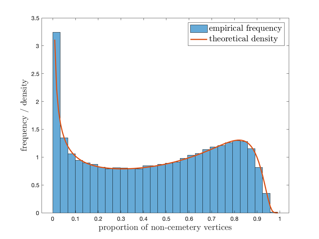
Figure 3: Normalized histogram of proportion of non-cemetery vertices in DEC, together with the theoretical limit density.

In Figure 3, we compare the empirical distribution of non-cemetery vertices and its limit density given by Corollary 5. In the simulation, we fix $\sigma=r=2$ and $n=100$, and randomly generate 10,000 rules.

5.4 Completion of proof of the main theorem

We now put together the results from Sections 3, 4, 5.2, and 5.3.

Proof of Theorem 1.

Recall the geometric random variable $K_{\sigma}$ from Section 3. For any $\epsilon>0$, pick $k_{\epsilon}$ large enough such that $\mathbb{P}\left(K_{\sigma}>k_{\epsilon}\right)<\epsilon$. Then we have

$$\mathbb{P}\left(\frac{X_{\sigma,n}}{n^{\sigma/2}}\leq x\right) =\mathbb{P}\left(n^{-\sigma/2}\max\left\{L_{i}\cdot T_{i},i=1,2,\dots\right\}\leq x\right)$$

$$\leq\sum_{k=1}^{k_{\epsilon}}\mathbb{P}\left(n^{-\sigma/2}\max\left\{L_{i}\cdot T_{i},i=1,2,\dots\right\}\leq x\bigm{|}K_{\sigma}=k\right)\mathbb{P}\left(K_{\sigma}=k\right)+\epsilon$$

$$=\sum_{k=1}^{k_{\epsilon}}\mathbb{P}\left(n^{-\sigma/2}\max\left\{L_{i}\cdot T_{i}^{\prime},L_{k}\sigma,i=1,2,\dots,k-1\right\}\leq x\right)\mathbb{P}\left(K_{\sigma}=k\right)+\epsilon$$

$$=\sum_{k=1}^{k_{\epsilon}}\mathbb{P}\left(\frac{D_{C_{n}}^{(k)}}{\sqrt{C_{n}}}\cdot\sqrt{\frac{C_{n}}{N}}\cdot\frac{\sqrt{N}}{n^{\sigma/2}}\leq x\right)\mathbb{P}\left(K_{\sigma}=k\right)+\epsilon,$$

where $D$ is defined in Lemma 4.4. Therefore, it suffices to show that

$$\mathbb{P}\left(\frac{D_{C_{n}}^{(k)}}{\sqrt{C_{n}}}\cdot\sqrt{\frac{C_{n}}{N}}\leq x\right)$$

converges as $n\to\infty$, for each fixed $k$. To this end, we partition the interval $(0,1]$ into $M$ sub-intervals, and write

(7) $$\mathbb{P}\left(\frac{D_{C_{n}}^{(k)}}{\sqrt{C_{n}}}\sqrt{\frac{C_{n}}{N}}\leq x\right)$$

$$=\sum_{i=0}^{M-1}\mathbb{P}\left(\frac{D_{C_{n}}^{(k)}}{\sqrt{N}}\leq x\biggm{|}\sqrt{\frac{C_{n}}{N}}\in\left(\frac{i}{M},\frac{i+1}{M}\right]\right)\mathbb{P}\left(\sqrt{\frac{C_{n}}{N}}\in\left(\frac{i}{M},\frac{i+1}{M}\right]\right).$$

Assume that $\sigma$ is even and let $a=1/\sqrt{\sigma}$. By Theorem 2,

(8) $$\mathbb{P}\left(\sqrt{\frac{C_{n}}{N}}\in\left(\frac{i}{M},\frac{i+1}{M}\right]\right)\to\int_{i/M}^{(i+1)/M}g_{\sqrt{1-\tau_{a}}}(t)\,dt,$$

as $n\to\infty$. Moreover,

(9) $$\mathbb{P}\left(\frac{D_{C_{n}}^{(k)}}{\sqrt{N}}\leq x\biggm{|}\sqrt{\frac{C_{n}}{N}}\in\left(\frac{i}{M},\frac{i+1}{M}\right]\right)\leq\mathbb{P}\left(\frac{D_{\lfloor i^{2}N/M^{2}\rfloor}^{(k)}}{\sqrt{N}i/M}\leq\frac{x}{i/M}\right).$$

It now follows from (7)-(9) and Lemma 4.4 that

$$\limsup_{n\to\infty}\mathbb{P}\left(\frac{D_{C_{n}}^{(k)}}{\sqrt{N}}\leq x\right) \leq\sum_{i=0}^{M-1}\mathbb{P}\left(D^{(k)}\leq\frac{x}{i/M}\right)\int_{i/M}^{(i+1)/M}g_{\sqrt{1-\tau_{a}}}(t)\,dt$$

$$=\sum_{i=0}^{M-1}\left[\mathbb{P}\left(D^{(k)}\leq\frac{x}{i/M}\right)\left(g_{\sqrt{1-\tau_{a}}}\left(\frac{i}{M}\right)\frac{1}{M}+\mathcal{O}\left(\frac{1}{M^{2}}\right)\right)\right]$$

$$\to\int_{0}^{1}\mathbb{P}\left(D^{(k)}\leq\frac{x}{y}\right)g_{\sqrt{1-\tau_{a}}}(y)\,dy$$

as $M\to\infty$, where $g_{\sqrt{1-\tau_{a}}}$ is the density of the random variable $\sqrt{1-\tau_{a}}$. The same lower bound for $\liminf_{n\to\infty}\mathbb{P}\left(\frac{D_{C_{n}}^{(k)}}{\sqrt{N}}\leq x\right)$ is obtained along similar lines. For odd $\sigma$, a simpler argument shows that

$$\lim_{n\to\infty}\mathbb{P}\left(\frac{D_{C_{n}}^{(k)}}{\sqrt{N}}\leq x\right)=\mathbb{P}\left(D^{(k)}\leq x\right),$$

and ends the proof. ∎

6 Conclusions and open problems

In a CA, finding PS of a given temporal period reduces to finding cycles of the corresponding DEC. When a rule is chosen at random, the arcs of the DEC are independent from each other, provided that the spatial period is less than the number of neighbors, i.e., if $\sigma\leq r$. The problem then reduces to finding the longest of the expanded cycles after the cemetery vertices have been eliminated.

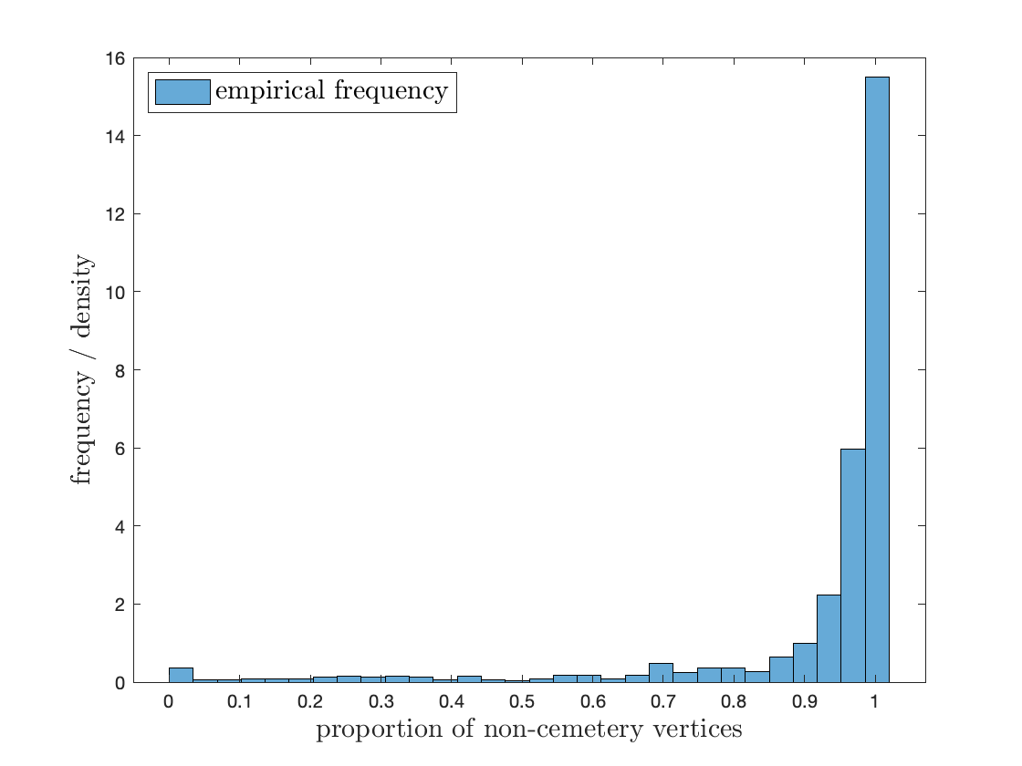
(a) $\sigma=3$, $r=2$

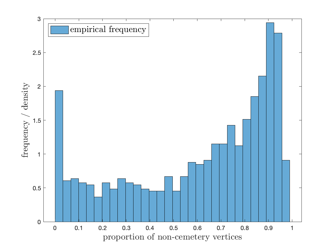
(b) $\sigma=4$, $r=2$

Figure 4: Empirical proportion of non-cemetery vertices for two examples with $r<\sigma$ and $n=50$, from $1000$ samples.

When $\sigma>r$, the independence among arcs in the DEC fails. For example, when $r=2$ and $\sigma=3$, the events $\{123\searrow a_{1}a_{2}a_{3}\}$ and $\{124\searrow b_{1}b_{2}b_{3}\}$ are dependent (as they cannot occur simultaneously unless $a_{2}=b_{2}$), but they are independent when $r=3$. Even though rigorous analysis seems elusive in this case, simulations strongly suggest that results very much like Theorems 1 and 2 hold. For starters, the random variable $C_{n}$ and the cemetery vertices in a DEC may be defined in the same manner, and they have the same connection to each other. Figure 4 supports the following conjecture.

Conjecture 6.1.

Fix arbitrary $\sigma,r\geq 1$, and let $n\to\infty$. If $\sigma$ is odd, $n^{-\sigma}C_{n}\to 1$ in probability. If $\sigma$ is even, then $n^{-\sigma}C_{n}$ converges in distribution to a nontrivial bimodal distribution.

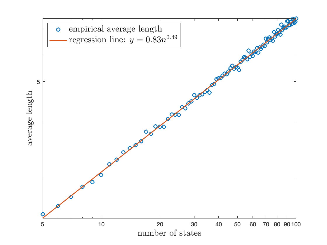
(a) $\sigma=1$, $r=2$, $5\leq n\leq 100$

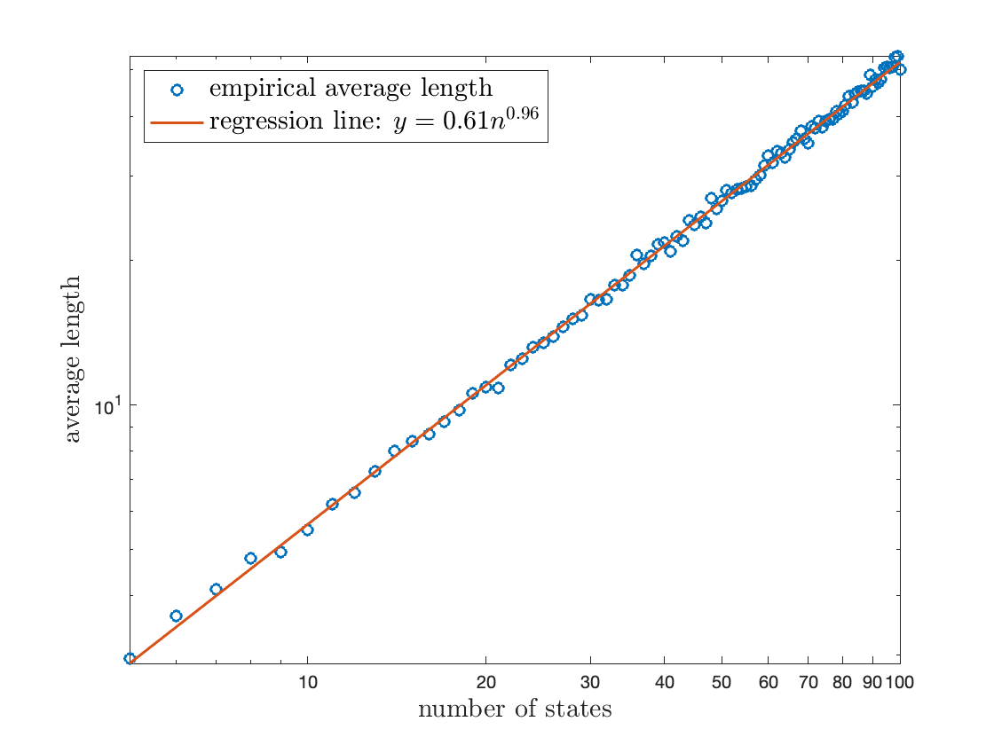
(b) $\sigma=2$, $r=2$, $5\leq n\leq 100$

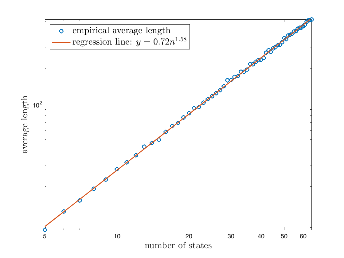
(c) $\sigma=3$, $r=2$, $5\leq n\leq 65$

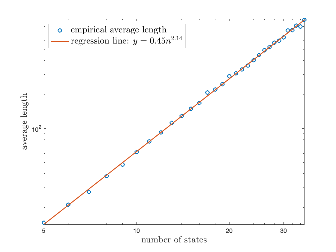
(d) $\sigma=4$, $r=2$, $5\leq n\leq 36$

Figure 5: Loglog plots of average lengths of longest PS with varied $\sigma$, from 1000 samples, with corresponding regression lines.

Turning to the longest periods themselves, we provide the loglog plots for $r=2$, and $\sigma=1,2,3,4$ in Figure 5. The first two cases are covered by Theorem 1, while the other two are not. Nevertheless, the average lengths behave with the same regularity, leading to our next conjecture.

Conjecture 6.2.

Theorem 1 holds in the same form for $\sigma>r$, i.e., $\displaystyle\frac{X_{\sigma,n}}{n^{\sigma/2}}$ converges in distribution, for any fixed $\sigma\geq 1$ and $r\geq 1$.

Returning to the case $\sigma\leq r$, one may ask whether our results can be extended to cover other than longest periods. Indeed, as we now sketch, it is possible to show that the length of the $j$th longest PS of a random rule, again scaled by $n^{\sigma/2}$ converges in distribution. To be more precise, recalling notation from Section 3, identify recursively for $\ell\geq 1$ the cycles with largest possible expansion numbers as follows: $K_{\sigma}^{(0)}=0$ and

$$K_{\sigma}^{(\ell)}=\min\left\{k>K_{\sigma}^{(\ell-1)}:T_{k}=\sigma\right\}.$$

Then the length of $j$th longest PS is given by

$$X_{\sigma,n}^{(j)}=\max_{(j)}\left\{L_{i}\cdot T_{i}^{\prime},L_{K_{\sigma}^{(\ell)}}\sigma:i=1,2,\dots,K_{\sigma}^{(j)}-1,i\neq K_{\sigma}^{(\ell)},\ell=1,\dots,j\right\},$$

where $\max_{(j)}$ returns the $j$th largest element of a set. The arguments similar to those in Sections 4 and 5.4, then show that $X_{\sigma,n}^{(j)}/n^{\sigma/2}$ converges in distribution to a nontrivial limit.

We conclude with four questions on the extensions of our results in different directions, some of which are analogous to the those posed in [14].

Question 6.3.

Assume that $n$ is fixed, but $\sigma,r\to\infty$. What is the asymptotic behavior of the longest temporal period with spatial period $\sigma$, depending on the relative sizes of $\sigma$ and $r$?

Question 6.4.

For a fixed $\tau$, define the random variable $X_{\tau,n}^{\prime}$ to be the longest spatial period of a PS with for a given temporal period $\tau$. What is the asymptotic behavior, as $n\to\infty$, of $X_{\tau,n}^{\prime}$?

A rule is left permutative if the map $\psi_{b_{-r+1},\ldots,b_{-1}}:\mathbb{Z}_{n}\to\mathbb{Z}_{n}$ given by $\psi_{b_{-r+1},\ldots,b_{-1}}(a)=f(b_{-r+1},\ldots,b_{-1},a)$ is a permutation for every $(b_{-r+1},\ldots,b_{-1})\in\mathbb{Z}_{n}^{r-1}$.

Question 6.5.

Let $\mathcal{L}$ be the set of all $(n!)^{n^{r-1}}$ left permutative rules. What is the asymptotic behavior of $X_{\sigma,n}$ if a rule from $\mathcal{L}$ is chosen uniformly at random?

Our final question is on additive rules [23], given by $f(b_{-r+1},\ldots,b_{0})=\sum_{i=-r+1}^{0}\beta_{i}b_{i}$, for some $\beta_{i}\in\mathbb{Z}_{n}$.

Question 6.6.

Let $\mathcal{A}$ be the set of all $n^{r}$ additive rules. What is the asymptotic behavior of $X_{\sigma,n}$ if a rule from $\mathcal{A}$ is chosen uniformly at random?

References

• [1] David J. Aldous, Grégory Miermont, and Jim Pitman. Brownian bridge asymptotics for random p-mappings. Electronic Journal of Probability, 9(paper no. 3):37–56, 2004.
• [2] David J. Aldous and Jim Pitman. Brownian bridge asymptotics for random mappings. Random Structures & Algorithms, 5(4):487–512, 1994.
• [3] Richard Arratia, Andrew D Barbour, and Simon Tavaré. Logarithmic combinatorial structures: a probabilistic approach, volume 1. European Mathematical Society, 2003.
• [4] Richard Arratia and Simon Tavaré. Limit theorems for combinatorial structures via discrete process approximations. Random Structures & Algorithms, 3(3):321–345, 1992.
• [5] Béla Bollobás. Random graphs. Number 73. Cambridge university press, 2001.
• [6] Mike Boyle and Bruce Kitchens. Periodic points for onto cellular automata. Indagationes Mathematicae, 10(4):483–493, 1999.
• [7] Mike Boyle and Bryant Lee. Jointly periodic points in cellular automata: computer explorations and conjectures. Experimental Mathematics, 16(3):293–302, 2007.
• [8] Kevin Cattell, Frank Ruskey, Joe Sawada, Micaela Serra, and C. Robert Miers. Fast algorithms to generate necklaces, unlabeled necklaces, and irreducible polynomials over gf (2). Journal of Algorithms, 37(2):267–282, 2000.
• [9] Taejoo Chang, Iickho Song, Jinsoo Bae, and Kwang Soon Kim. Maximum length cellular automaton sequences and its application. Signal Processing, 56(2):199–203, 1997.
• [10] Sourav Das and Dipanwita Roy Chowdhury. Generating cryptographically suitable non-linear maximum length cellular automata. In International Conference on Cellular Automata, pages 241–250. Springer, 2010.
• [11] Philippe Flajolet and Andrew M. Odlyzko. Random mapping statistics. In Workshop on the Theory and Application of of Cryptographic Techniques, pages 329–354. Springer, 1989.
• [12] Janko Gravner and David Griffeath. Robust periodic solutions and evolution from seeds in one-dimensional edge cellular automata. Theoretical Computer Science, 466:64, 2012.
• [13] Janko Gravner and Xiaochen Liu. Maximal temporal period of a periodic solution generated by a one-dimensional cellular automaton. In preparation, 2019.
• [14] Janko Gravner and Xiaochen Liu. Periodic solutions of one-dimensional cellular automata with random rules. In preparation, 2019.
• [15] Jennie C. Hansen and Jerzy Jaworski. Compound random mappings. Journal of applied probability, 39(4):712–729, 2002.
• [16] Erica Jen. Global properties of cellular automata. Journal of Statistical Physics, 43(1–2):219–242, 1986.
• [17] Erica Jen. Cylindrical cellular automata. Communications in Mathematical Physics, 118(4):569–590, 1988.
• [18] Erica Jen. Linear cellular automata and recurring sequences in finite fields. Communications in Mathematical Physics, 119(1):13–28, 1988.
• [19] Ionannis Karatzas and Steven Shreve. Brownian Motion and Stochastic Calculus. Springer, New York, 2nd edition, 1998.
• [20] Jae-Gyeom Kim. On state transition diagrams of cellular automata. East Asian Math. J, 25(4):517–525, 2009.
• [21] Andreas Knoblauch. Closed-form expressions for the moments of the binomial probability distribution. SIAM Journal on Applied Mathematics, 69(1):197–204, 2008.
• [22] Harold J. Kushner. On the weak convergence of interpolated markov chains to a diffusion. The annals of Probability, pages 40–50, 1974.
• [23] Olivier Martin, Andrew M. Odlyzko, and Stephen Wolfram. Algebraic properties of cellular automata. Communications in mathematical physics, 93(2):219–258, 1984.
• [24] Michał Misiurewicz, John G. Stevens, and Diana M. Thomas. Iterations of linear maps over finite fields. Linear algebra and its applications, 413(1):218–234, 2006.
• [25] Eduard Reithmeier. Periodic Solutions of Nonlinear Dynamical Systems. Springer-Verlag, 1991.
• [26] John G. Stevens. On the construction of state diagrams for cellular automata with additive rules. Information Sciences, 115(1-4):43–59, 1999.
• [27] John G. Stevens, Ronald E. Rosensweig, and A. E. Cerkanowicz. Transient and cyclic behavior of cellular automata with null boundary conditions. Journal of statistical physics, 73(1-2):159–174, 1993.
• [28] Stephen Wolfram. Computation theory of cellular automata. Communications in mathematical physics, 96(1):15–57, 1984.
• [29] Stephen Wolfram. Random sequence generation by cellular automata. Advances in Applied Mathematics, 7(2):132–169, 1986.
• [30] Stephen Wolfram. A new kind of science, volume 5. Wolfram media Champaign, IL, 2002.
• [31] Xu Xu, Yi Song, and Stephen P. Banks. On the dynamical behavior of cellular automata. International Journal of Bifurcation and Chaos, 19(04):1147–1156, 2009.