A class of partition functions associated with $E_{\tau,\eta}(gl_{3})$
by Izergin-Korepin analysis

Abstract

Recently, a class of partition functions associated with higher rank rational and trigonometric integrable models were introduced by Foda and Manabe. We use the dynamical $R$-matrix of the elliptic quantum group $E_{\tau,\eta}(gl_{3})$ to introduce an elliptic analogue of the partition functions associated with $E_{\tau,\eta}(gl_{3})$. We investigate the partition functions of Foda-Manabe type by developing a nested version of the elliptic Izergin-Korepin analysis, and present the explicit forms as symmetrization of multivariable elliptic functions. We show that special cases are essentially the elliptic weights functions introduced in the works by Rimányi-Tarasov-Varchenko, Konno, Felder-Rimányi-Varchenko.

1 Introduction

Partition functions of integrable models [1, 2, 3] in statistical physics have rich connections with mathematics and high energy physics. As for the connection with mathematics, one of the important facts is that wavefunctions of integrable models can be expressed using symmetric functions such as the Schur, Hall-Littlewood, Grothendieck polynomials and their symplectic analogues, $q$-deformation and elliptic generalizations. See [4, 5, 6, 7, 8, 9, 10, 11, 12, 13, 14, 15, 16, 17, 18, 19, 20, 21] for examples on various topics of investigations and applications of the correspondence between the wavefunctions and symmetric functions.

One of the challenging problems is to go beyond six-vertex models and study partition functions for higher rank models. See [22, 23, 24, 25, 26, 27, 28, 29, 30, 31] for examples on seminal and recent works on this topic. One of the recent progresses has been made by Foda and Manabe [32], which they introduced a new class of partition functions for higher rank rational and trigonometric models, motivated by the Bethe/Gauge correspondence [33, 34], and their partition functions seem to deserve further studies.

In this paper, we introduce and study an elliptic analogue of the partition functions of Foda-Manabe type associated with elliptic quantum group [35, 36, 37, 38] $E_{\tau,\eta}(gl_{3})$. We use the Izergin-Korepin method for the analysis of the partition functions. The Izergin-Korepin method is a method initiated by Korepin [39] and used by Izergin [40] to find a determinant representation for the domain wall boundary partition functions of the trigonometric six-vertex model. The determinant representation (Izegin-Korepin determinant) has found many applications and connections to many branches of mathematics and mathematical physics, such as the enumeration of the alternating sign matrices, relations with orthogonal polynomials and classical integrable systems [41, 42, 43, 44, 45, 46, 47, 48, 49]. The Izergin-Korepin method was also applied to variants of the domain wall boundary partition functions and extended to the scalar products [42, 43, 50, 51]. There are also developments on the studies of the domain wall boundary partition functions for elliptic integrable models by various methods. See [23, 52, 53, 54, 55, 56, 57, 58, 59, 60] for examples on this topic.

Recently, for the case of six-vertex type models, the Izergin-Korepin method was extended to the wavefunctions [61, 62], and we develop a nested version of this method in this paper for the purpose of analyzing the partition functions of Foda-Manabe type. We use the Izergin-Korepin method in two steps. We first use the method to analyze partition functions which we call as the base partition functions, which is essentially partition functions associated with $E_{\tau,\eta}(gl_{2})$. We next perform the Izergin-Korepin analysis on the partition functions of Foda-Manabe type associated with $E_{\tau,\eta}(gl_{3})$. The Izergin-Korepin method is a method which uses graphical representations of integrable models to construct relations between partition functions of different sizes. One needs the intitial condition, and the base partition functions essentially serve as the initial condition for the second Izergin-Korepin analysis. This is similar to the Izergin-Korepin analysis on the scalar products by Wheeler [51], which he introduced intermediate scalar products as a generalization, and the initial condition of the Izergin-Korepin analysis for the intermediate scalar products is essentially given by the domain wall boundary partition functions. Foda and Manabe mention that the partition functions of rational and trigonometric models they introduced contain the nested wavefunctions as special cases. From the point of view of the Izergin-Korepin analysis, the relation between the partition functions they introduced and the nested wavefunctions resemble the relation between the intermediate scalar products and the scalar products, since one needs generalizations of the partition functions to investigate the original ones. We also show that special cases are essentially the elliptic weights functions introduced in the works by Rimányi-Tarasov-Varchenko, Konno, Felder-Rimányi-Varchenko [63, 64, 65, 66], which appear as objects in the integral representation of the solutions to the elliptic $q$-KZ equations, and also essentially play the role of elliptic stable envelope maps for the cotangent bundles of flag varieties, which are geometric objects originally proposed by Aganagic-Okounkov [67] as an elliptic generalization of the cohomological stable envelopes which appear in the works by Maulik-Okounkov [68], in which they initiated a program to relate quantum torus equivariant cohomology of quiver varieties and representation theory of quantum groups, which is considered as a mathematical formulation of the Bethe/gauge correspondence [33, 34].

This paper is organized as follows. In the next section, we introduce the dynamical $R$-matrix and list the properties of theta functions which are necessary for the present paper. In section 3, we introduce two types of partition functions: the base partition functions and partition functions of Foda-Manabe type. In section 4, we analyze the base partition functions. In section 5, we perform the Izergin-Korepin analysis on partition functions of Foda-Manabe type, and determine the explicit form of the partition functions. In section 6, we show that special cases of the elliptic partition functions of Foda-Manabe type are the elliptic weights functions studied in Rimányi-Tarasov-Varchenko, Konno, Felder-Rimányi-Varchenko. Section 7 is devoted to the conclusion of this paper.

2 Theta function and Dynamical $R$-matrix

In this section, we recall the properties of the theta functions and the dynamical $R$-matrix which we use in this paper.

First we introduce the theta function

$$[z]=-\sum_{j\in{\bf Z}+1/2}e^{i\pi j^{2}\tau+2\pi ij(z+1/2)},$$ (2.1)

which is an odd function $[-z]=-[z]$ and satisfy the quasi-periodicities

$$[z+1] =-[z],$$ (2.2)

$$[z+\tau] =-e^{-2\pi iz-\pi i\tau}[z].$$ (2.3)

For the elliptic version of the Izergin-Korepin analysis, we use the following facts about the elliptic polynomials [52, 69].

A character is a group homomorphism $\chi$ from multiplicative groups $\Gamma=\mathbf{Z}+\tau\mathbf{Z}$ to $\mathbf{C}^{\times}$. An $n$-dimensional space $\Theta_{n}(\chi)$ is defined for each character $\chi$ and positive integer $n$, which consists of holomorphic functions $\phi(y)$ on $\mathbf{C}$ satisfying the quasi-periodicities

$$\phi(y+1) =\chi(1)\phi(y),$$ (2.4)

$$\phi(y+\tau) =\chi(\tau)e^{-2\pi iny-\pi in\tau}\phi(y).$$ (2.5)

The elements of the space $\Theta_{n}(\chi)$ are called elliptic polynomials. The space $\Theta_{n}(\chi)$ is $n$-dimensional [52, 69] and the following fact holds for the elliptic polynomials.

Proposition 2.1.

[52, 69] Suppose there are two elliptic polynomials $P(y)$ and $Q(y)$ in $\Theta_{n}(\chi)$, where $\chi(1)=(-1)^{n}$, $\chi(\tau)=(-1)^{n}e^{\alpha}$. If those two polynomials are equal $P(y_{j})=Q(y_{j})$ at $n$ points $y_{j}$, $j=1,\dots,n$ satisfying $y_{j}-y_{k}\not\in\Gamma$, $\sum_{k=1}^{N}y_{k}-\alpha\not\in\Gamma$, then the two polynomials are exactly the same $P(y)=Q(y)$.

The above proposition is an elliptic analogue of the following properties for ordinary polynomials: if $P(y)$ and $Q(y)$ are polynomials of degree $n-1$ in $y$, and if these polynomials match at $n$ distinct points, then the two polynomials are exactly the same. These properties ensure the uniqueness of the Izergin-Korepin analysis, which was effectively used in [52] to study the domain wall boundary partition functions of the Andrews-Baxter-Forrester model [70] which is related to the eight-vertex model [71] by the vertex-face transformation.

Next, let us reall the dynamical $R$-matrix. We use the dynamical $R$-matrix for the face-type elliptic quantum group $E_{\tau,\eta}(gl_{n})$ [35, 36, 37, 38] (there are also vertex-type and centrally-extended versions of the elliptic quantum groups [72, 73, 74, 75]). The dynamical $R$-matrix for the elliptic quantum group $E_{\tau,\eta}(gl_{n})$ is a function $R(z,\lambda):{\bf C}\otimes\mathfrak{h}^{*}\longrightarrow\mathrm{End}(V\otimes V)$ where $\mathfrak{h}$ is a Cartan subalgebra of $gl_{n}$, $\mathfrak{h}^{*}$ is its dual and $V$ is a diagonalizable $\mathfrak{h}$-module. For the case we consider, $V$ is the $\mathfrak{h}$-module ${\bf C}^{n}$ with standard basis $e_{i},i=1,\dots,n$. Let us define $\mu_{i}\in\mathfrak{h}^{*}$ as $\mu_{i}(h)=h^{i}$ if $h=\mathrm{diag}(h^{1},\dots,h^{n})\in\mathfrak{h}$. Then $V=\oplus_{i=1}^{N}V^{\mu_{i}}$ where $V^{\mu_{i}}={\bf C}e_{i}$.

The explicit form of the dynamical $R$-matrix is given by

$$R(z,\lambda)=\sum_{i=1}^{N}[z-\gamma]E_{ii}\otimes E_{ii}+\sum_{i\neq j}\alpha(z,\lambda_{i}-\lambda_{j})E_{ii}\otimes E_{jj}+\sum_{i\neq j}\beta(z,\lambda_{i}-\lambda_{j})E_{ij}\otimes E_{ji},$$ (2.6)

where $E_{ij}$ are matrix units $E_{ij}e_{k}=\delta_{jk}e_{i}$. $\alpha(z,\lambda)$ and $\beta(z,\lambda)$ are given in terms of theta functions as

$$\alpha(z,\lambda)=\frac{[z][\lambda+\gamma]}{[\lambda]},\ \beta(z,\lambda)=-\frac{[z+\lambda][\gamma]}{[\lambda]},$$ (2.7)

and $\lambda_{i}$ in (2.6) are coordinate functions $\lambda_{i}=\lambda(E_{ii}),i=1,\dots,n$.

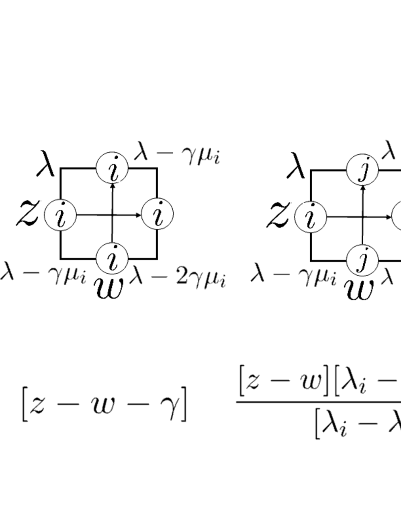
Figure 1: A graphical description of the dynamical $R$-matrix $R(z-w,\lambda)$ (2.6). Here, $i$ and $j$ are different $i\neq j$.

The dynamical $R$-matrix (2.6) satisfies the dynamical Yang-Baxter relation

$$R_{23}(z_{2}-z_{3},\lambda)R_{13}(z_{1}-z_{3},\lambda-\gamma h_{2})R_{12}(z_{1}-z_{2},\lambda)$$

$$= R_{12}(z_{1}-z_{2},\lambda-\gamma h_{3})R_{13}(z_{1}-z_{3},\lambda)R_{23}(z_{1}-z_{3},\lambda-\gamma h_{1}),$$ (2.8)

acting on $V_{1}\otimes V_{2}\otimes V_{3}$. The subscripts indicate the spaces the operators are acting on. For example,

$$R_{12}(z_{1}-z_{2},\lambda-\gamma h_{3})(v_{1}\otimes v_{2}\otimes v_{3})=R(z_{1}-z_{2},\lambda-\gamma\alpha)v_{1}\otimes v_{2}\otimes v_{3},$$ (2.9)

if $v_{3}\in V^{\alpha}$.

The dynamical $R$-matrix has its origin in the elliptic face model [70, 76, 77], and it describes the face model like a six-vertex model with an additional dynamical parameter. The dynamical $R$-matrix $R(z-w,\lambda)$ can be expressed as Figure 1 for example. We use this graphical description of the dynamical $R$-matrix to construct and study partition functions.

3 Partition functions

We introduce two types of partition functions in this section: the base partition functions and an elliptic analogue of the partition functions introduced by Foda and Manabe [32] recently.

First, we introduce monodromy matrix as

$$T_{a}(z|w_{1},\dots,w_{L}|\lambda)$$

$$= R_{aL}(z-w_{L},\lambda-\gamma(h_{1}+\cdots+h_{L-1}))\cdots R_{a2}(z-w_{2},\lambda-\gamma h_{1})R_{a1}(z-w_{1},\lambda),$$ (3.1)

acting on $V_{a}\otimes(V_{1}\otimes\cdots\otimes V_{L})$. We also use bra-ket notations. We denote the basis vector $e_{i}$ on $V_{j}$ as $|i\rangle_{j}$ and its dual $e_{i}^{*}$ as ${}_{j}\langle i|$.

We now introduce the following partition functions (Figure 2)

Figure 2: The base partition functions $W_{L,k}(z_{1},\dots,z_{k}|w_{1},\dots,w_{L}|I_{1},\dots,I_{k}|\lambda)$ (3.2).

$$W_{L,k}(z_{1},\dots,z_{k}|w_{1},\dots,w_{L}|I_{1},\dots,I_{k}|\lambda)$$

$$= {}_{a_{1}}\langle 2|\otimes\cdots\otimes{}_{a_{k}}\langle 2|\otimes{}_{1}\langle i_{1}^{(1)}|\otimes\cdots\otimes{}_{L}\langle i_{L}^{(1)}|$$

$$T_{a_{1}}(z_{1}|w_{1},\dots,w_{L}|\lambda)T_{a_{2}}(z_{2}|w_{1},\dots,w_{L}|\lambda-\gamma h_{a_{1}})\cdots$$

$$\cdots T_{a_{k}}(z_{k}|w_{1},\dots,w_{L}|\lambda-\gamma(h_{a_{1}}+\cdots h_{a_{k-1}}))|1\rangle_{a_{1}}\otimes\cdots\otimes|1\rangle_{a_{k}}\otimes|2\rangle_{1}\otimes\cdots\otimes|2\rangle_{L},$$ (3.2)

where $i_{j}^{(1)}$ ($j=1,\dots,L$) is 1 if $j=I_{\ell}$ for some $\ell\in\{1,\dots,k\}$, and 2 otherwise. In this paper, we call the partition functions $W_{L,k}(z_{1},\dots,z_{k}|w_{1},\dots,w_{L}|I_{1},\dots,I_{k}|\lambda)$ as the base partition functions. Note that only matrix elements of the form ${}_{1}\langle j_{1}|{}_{2}\langle j_{2}|R_{12}(z-w,\lambda)|i_{1}\rangle_{1}|i_{2}\rangle_{2}$, $i_{1},i_{2},j_{1},j_{2}=1,2$ contribute to the base partition functions, i.e. the base partition functions are essentially partition functions associated with $E_{\tau,\eta}(gl_{2})$.

Next we introduce a class of partition functions associated with $E_{\tau.\eta}(gl_{3})$, which is an elliptic analogue of the one recently introduced by Foda and Manabe [32]. Let us denote

$$T_{a}(z|\{\bm{z}^{(2)}\},\{\bm{w}^{(1)}\}|\lambda)$$

$$= R_{a,k_{2}+L_{1}}(z-w_{L_{1}}^{(1)},\lambda-\gamma(h_{1}+\cdots+h_{k_{2}+L_{1}-1}))\cdots R_{a,k_{2}+1}(z-w_{1}^{(1)},\lambda-\gamma(h_{1}+\cdots+h_{k_{2}}))$$

$$\times R_{ak_{2}}(z-z_{k_{2}}^{(2)},\lambda-\gamma(h_{1}+\cdots+h_{k_{2}-1}))\cdots R_{a1}(z-z_{1}^{(2)},\lambda),$$ (3.3)

The partition functions we consider is (Figure 3)

Figure 3: The partition functions of Foda-Manabe type associated with $E_{\tau,\eta}(gl_{3})$ $W(\{{\bm{z}^{(1)}}\},\{{\bm{z}^{(2)}}\}|\{{\bm{w}^{(1)}}\},\{{\bm{w}^{(2)}}\}|\{k_{1},k_{2},L_{1},L_{2},{\bm{I}}\}|\lambda)$ (3.4).

$$W(\{{\bm{z}^{(1)}}\},\{{\bm{z}^{(2)}}\}|\{{\bm{w}^{(1)}}\},\{{\bm{w}^{(2)}}\}|\{k_{1},k_{2},L_{1},L_{2},{\bm{I}}\}|\lambda)$$

$$= \sum_{\ell_{1},\dots,\ell_{k_{2}}=1,2}{}_{a_{1}}\langle 3|\otimes\cdots\otimes{}_{a_{k_{2}}}\langle 3|\otimes{}_{1}\langle i_{1}^{(2)}|\otimes\cdots\otimes{}_{L_{2}}\langle i_{L_{2}}^{(2)}|$$

$$T_{a_{1}}(z_{1}^{(2)}|w_{1}^{(2)},\dots,w_{L_{2}}^{(2)}|\lambda)T_{a_{2}}(z_{2}^{(2)}|w_{1}^{(2)},\dots,w_{L_{2}}^{(2)}|\lambda-\gamma h_{a_{1}})\cdots$$

$$\cdots T_{a_{k_{2}}}(z_{k_{2}}^{(2)}|w_{1}^{(2)},\dots,w_{L_{2}}^{(2)}|\lambda-\gamma(h_{a_{1}}+\cdots+h_{a_{{k_{2}}-1}}))|\ell_{1}\rangle_{a_{1}}\otimes\cdots\otimes|\ell_{k_{2}}\rangle_{a_{k_{2}}}\otimes|3\rangle_{1}\otimes\cdots\otimes|3\rangle_{L_{2}}$$

$$\times {}_{a_{1}}\langle 2|\otimes\cdots\otimes{}_{a_{k_{1}}}\langle 2|\otimes{}_{1}\langle\ell_{1}|\otimes\cdots\otimes{}_{k_{2}}\langle\ell_{k_{2}}|\otimes{}_{k_{2}+1}\langle i_{1}^{(1)}|\otimes\cdots\otimes{}_{k_{2}+L_{1}}\langle i_{L_{1}}^{(1)}|$$

$$T_{a_{1}}(z_{1}^{(1)}|\{{\bm{z}^{(2)}}\},\{{\bm{w}^{(1)}}\}|\lambda)T_{a_{2}}(z_{2}^{(1)}|\{{\bm{z}^{(2)}}\},\{{\bm{w}^{(1)}}\}|\lambda-\gamma h_{a_{1}})\cdots$$

$$\cdots T_{a_{k_{1}}}(z_{k_{1}}^{(1)}|\{{\bm{z}^{(2)}}\},\{{\bm{w}^{(1)}}\}|\lambda-\gamma(h_{a_{1}}+\cdots+h_{a_{{k_{1}}-1}}))|1\rangle_{a_{1}}\otimes\cdots\otimes|1\rangle_{a_{k_{1}}}\otimes|2\rangle_{1}\otimes\cdots\otimes|2\rangle_{k_{2}+L_{1}}.$$ (3.4)

The partition functions $W(\{{\bm{z}^{(1)}}\},\{{\bm{z}^{(2)}}\}|\{{\bm{w}^{(1)}}\},\{{\bm{w}^{(2)}}\}|\{k_{1},k_{2},L_{1},L_{2},{\bm{I}}\}|\lambda)$ depend on the sets of parameters $\{{\bm{z}^{(1)}}\}=\{z_{1}^{(1)},\dots,z_{k_{1}}^{(1)}\}$, $\{{\bm{z}^{(2)}}\}=\{z_{1}^{(1)},\dots,z_{k_{2}}^{(2)}\}$, $\{{\bm{w}^{(1)}}\}=\{w_{1}^{(1)},\dots,w_{L_{1}}^{(1)}\}$ $\{{\bm{w}^{(2)}}\}=\{w_{1}^{(2)},\dots,w_{L_{2}}^{(2)}\}$. The partition functions of Foda-Manabe type also depend on “the configuration of colors” $i_{1}^{(1)},\dots,\dots,i_{L_{1}}^{(1)}\in\{1,2\}$, $i_{1}^{(2)},\dots,\dots,i_{L_{2}}^{(2)}\in\{1,2,3\}$.

We adopt the label introduced by Foda-Manabe to label the configurations. A configuration of colors is labeled by a set ${\bm{I}}:=\{{\bm{I}_{k_{1}}^{(1)}},{\bm{I}_{k_{2}}^{(2)}},\widehat{{\bm{I}}}_{k_{2}+L_{1}}^{(2)},\widehat{{\bm{I}}}_{L_{2}}^{(3)}\}$ where the subsets ${\bm{I}_{k_{1}}^{(1)}},{\bm{I}_{k_{2}}^{(2)}},\widehat{{\bm{I}}}_{k_{2}+L_{1}}^{(2)},\widehat{{\bm{I}}}_{L_{2}}^{(3)}$ satisfy the following relations

$${\bm{I}}_{k_{1}}^{(1)}\subset\widehat{{\bm{I}}}_{k_{2}+L_{1}}^{(2)}:={\bm{I}_{k_{2}}^{(2)}}\cup\{L_{2}+1,\dots,L_{2}+L_{1}\},$$ (3.5)

$${\bm{I}_{k_{2}}^{(2)}}\subset\widehat{{\bm{I}}}_{L_{2}}^{(3)}:=\{1,\dots,L_{2}\}.$$ (3.6)

The relation between the naive label $i_{1}^{(1)},\dots,\dots,i_{L_{1}}^{(1)}$, $i_{1}^{(2)},\dots,\dots,i_{L_{2}}^{(2)}$ for the configuration of colors and ${\bm{I}}=\{{\bm{I}_{k_{1}}^{(1)}},{\bm{I}_{k_{2}}^{(2)}},\widehat{{\bm{I}}}_{k_{2}+L_{1}}^{(2)},\widehat{{\bm{I}}}_{L_{2}}^{(3)}\}$ is as follows. We label the positions which have colors $i_{1}^{(2)},\dots,\dots,i_{L_{2}}^{(2)}$ as $1,2,\dots,L_{2}$, and positions which have colors $i_{1}^{(1)},\dots,\dots,i_{L_{1}}^{(1)}$ are labeled as $L_{2}+1,\dots,L_{1}+L_{2}$. ${\bm{I}}_{k_{2}}^{(2)}$ is a set such that $\widehat{{\bm{I}}}_{L_{2}}^{(3)}\backslash{\bm{I}_{k_{2}}^{(2)}}$ is the set of positions which have color $3$, and ${\bm{I}}_{k_{1}}^{(1)}$ is the set of positions which have color $1$ so that $\widehat{{\bm{I}}}_{k_{2}+L_{1}}^{(2)}\backslash{\bm{I}}_{k_{1}}^{(1)}$ becomes the set which records the positions of color $2$. Since the definition of the subsets of ${\bm{I}}$ depends on integers $k_{1},k_{2},L_{1},L_{2}$ which characterize the sizes of partition functions, we introduce the full label $\{k_{1},k_{2},L_{1},L_{2},{\bm{I}}\}$ for the configuration of colors. This full label is important for the Izergin-Korepin analysis for the partition functions of Foda-Manabe type. In this paper, we call the quadruplet $\{k_{1},k_{2},L_{1},L_{2}\}$ as the size of the partition functions. Also note that throughout this paper, when one denotes the set as ${\bm{I}}_{k}^{(b)}$, the number of elements of the set is $k$, and the elements of the set are denoted as $I_{1}^{(b)},\cdots,I_{k}^{(b)}$ where $I_{1}^{(b)}<\cdots<I_{k}^{(b)}$.

For later purpose, we also use the induced set $\widetilde{{\bm{I}_{k_{1}}^{(1)}}}$ which is induced by the map

$${\bm{I}}_{k_{1}}^{(1)}\subset\widehat{{\bm{I}}}_{k_{2}+L_{1}}^{(2)}\longrightarrow\widetilde{{\bm{I}_{k_{1}}^{(1)}}}\subset\{1,\dots,k_{2}+L_{1}\}.$$ (3.7)

We map the set $\widehat{{\bm{I}}}_{k_{2}+L_{1}}^{(2)}$ to $\{1,\dots,k_{2}+L_{1}\}$ by $\widehat{I}_{a}^{(2)}\longrightarrow a$ $(a=1,\dots,k_{2}+L_{1})$, and correspondingly the elements in ${\bm{I}}_{k_{1}}^{(1)}$ which are included in $\widehat{{\bm{I}}}_{k_{2}+L_{1}}^{(2)}$ are naturally mapped to elements in $\{1,\dots,k_{2}+L_{1}\}$, which form the induced subset $\widetilde{{\bm{I}_{k_{1}}^{(1)}}}$.

4 Base partition functions

In this section, we analyze the base partition functions $W_{L,k}(z_{1},\dots,z_{k}|w_{1},\dots,w_{L}|I_{1},\dots,I_{k}|\lambda)$ which is used as the initial condition for the Izergin-Korepin analysis [39, 40] on the partition functions of Foda-Manabe type $W(\{{\bm{z}^{(1)}}\},\{{\bm{z}^{(2)}}\}|\{{\bm{w}^{(1)}}\},\{{\bm{w}^{(2)}}\}|\{k_{1},k_{2},L_{1},L_{2},{\bm{I}}\}|\lambda)$ in the next section. The idea of the Izergin-Korepin analysis is to construct relations between partition functions of different sizes and determine the initial condition, and find the explicit forms satisfying the recursive relations and the initial condition. The base partition functions $W_{L,k}(z_{1},\dots,z_{k}|w_{1},\dots,w_{L}|I_{1},\dots,I_{k}|\lambda)$ serve as the initial condition for the Izergin-Korepin analysis on the partition functions $W(\{{\bm{z}^{(1)}}\},\{{\bm{z}^{(2)}}\}|\{{\bm{w}^{(1)}}\},\{{\bm{w}^{(2)}}\}|\{k_{1},k_{2},L_{1},L_{2},{\bm{I}}\}|\lambda)$. In this section, we analyze the base partition functions $W_{L,k}(z_{1},\dots,z_{k}|w_{1},\dots,w_{L}|I_{1},\dots,I_{k}|\lambda)$ itself by using the Izergin-Korepin method for the wavefunctions [61, 62]. First, we introduce the elliptic multivariable functions and state the correspondence with the base partition functions.

Definition 4.1.

We define symmetric functions $E_{L,k}(z_{1},\dots,z_{k}|w_{1},\dots,w_{L}|I_{1},\dots,I_{k}|\lambda)$ that depend on the symmetric variables $z_{1},\dots,z_{k}$, complex parameters $w_{1},\dots,w_{L}$, $\gamma$, $\lambda_{1},\lambda_{2}$ and integers $I_{1},\dots,I_{k}$ satisfying $1\leq I_{1}<\cdots<I_{k}\leq L$,

$$E_{L,k}(z_{1},\dots,z_{k}|w_{1},\dots,w_{L}|I_{1},\dots,I_{k}|\lambda)$$

$$= \frac{[\gamma]^{k}}{\prod_{j=1}^{k}[\lambda_{1}-\lambda_{2}+(1-j)\gamma]}\sum_{\sigma\in S_{k}}\prod_{a=1}^{k}\Bigg{(}[z_{\sigma(a)}-w_{I_{a}}+\lambda_{2}-\lambda_{1}+(2a-1-I_{a})\gamma]$$

$$\times \prod_{i=1}^{I_{a}-1}[z_{\sigma(a)}-w_{i}]\prod_{i=I_{a}+1}^{L}[z_{\sigma(a)}-w_{i}-\gamma]\Bigg{)}\prod_{1\leq a<b\leq k}\frac{[z_{\sigma(a)}-z_{\sigma(b)}+\gamma]}{[z_{\sigma(a)}-z_{\sigma(b)}]}.$$ (4.1)

Theorem 4.2.

The base partition functions $W_{L,k}(z_{1},\dots,z_{k}|w_{1},\dots,w_{L}|I_{1},\dots,I_{k}|\lambda)$ can be explicitly expressed as the symmetric functions $E_{L,k}(z_{1},\dots,z_{k}|w_{1},\dots,w_{L}|I_{1},\dots,I_{k}|\lambda)$,

$$W_{L,k}(z_{1},\dots,z_{k}|w_{1},\dots,w_{L}|I_{1},\dots,I_{k}|\lambda)=E_{L,k}(z_{1},\dots,z_{k}|w_{1},\dots,w_{L}|I_{1},\dots,I_{k}|\lambda).$$ (4.2)

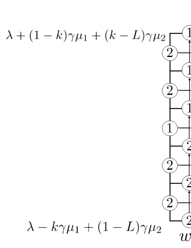
Figure 4: The states of the rightmost column of the partition functions $W_{L,k}(z_{1},\dots,z_{k}|w_{1},\dots,w_{L}|I_{1},\dots,I_{k}|\lambda)$ giving non-zero contributions are graphically represented as above. The factors including $w_{L}$ all come from the matrix elements of the dynamical $R$-matrices in this column and can be computed from the above graphical description. We get $\displaystyle g_{\ell}(w_{L})=[z_{\ell}-w_{L}+\lambda_{2}-\lambda_{1}+(2k-L-\ell)\gamma]\prod_{j=1}^{\ell-1}[z_{j}-w_{L}]\prod_{j=\ell+1}^{k}[z_{j}-w_{L}-\gamma],\ \ \ \ell=1,\cdots,k$.

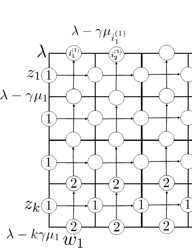
Figure 5: The base partition functions satisfying $I_{k}=L$, evaluated at $w_{L}=z_{k}-\gamma$ (4.5). The dynamical $R$-matrices at the rightmost column and the bottom row are all frozen.

Figure 6: The base partition functions with $I_{k}\neq L$ (4.6). The dynamical $R$-matrices at the rightmost column are all frozen.

We give below a proof of Theorem 4.2 by using the Izergin-Korepin method [39, 40] for the wavefunctions [61, 62]. See also [14, 37] which treat the same type of elliptic partition functions by different methods.

Proof.

First, we construct Korepin’s lemma, i.e. list the properties of the base partition functions which uniquely define them. For the case of partition functions of wavefunctions type, it is given by the following proposition.

Proposition 4.3.

The base partition functions $W_{L,k}(z_{1},\dots,z_{k}|w_{1},\dots,w_{L}|I_{1},\dots,I_{k}|\lambda)$ possess the following properties.

(1) If $I_{k}=L$, the base partition functions $W_{L,k}(z_{1},\dots,z_{k}|w_{1},\dots,w_{L}|I_{1},\dots,I_{k}|\lambda)$ are elliptic polynomials of $w_{L}$ in $\Theta_{k}(\chi)$ with quasi-periodicities

$$W_{L,k}(z_{1},\dots,z_{k}|w_{1},\dots,w_{L}+1|I_{1},\dots,I_{k}|\lambda)$$

$$= (-1)^{k}W_{L,k}(z_{1},\dots,z_{k}|w_{1},\dots,w_{L}|I_{1},\dots,I_{k}|\lambda),$$ (4.3)

$$W_{L,k}(z_{1},\dots,z_{k}|w_{1},\dots,w_{L}+\tau|I_{1},\dots,I_{k}|\lambda),$$

$$= (-1)^{k}\mathrm{exp}\Bigg{(}-2\pi i\Bigg{(}kw_{L}-\sum_{i=1}^{k}z_{i}+\lambda_{1}-\lambda_{2}+\gamma(L-k)\Bigg{)}-\pi ik\tau\Bigg{)}$$

$$\times W_{L,k}(z_{1},\dots,z_{k}|w_{1},\dots,w_{L}|I_{1},\dots,I_{k}|\lambda).$$ (4.4)

(2) The base partition functions $W_{L,k}(z_{1},\dots,z_{k}|w_{1},\dots,w_{L}|I_{1},\dots,I_{k}|\lambda)$ are symmetric with respect to $z_{1},\dots,z_{k}$.

(3) If $I_{k}=L$, the following recursive relations between the base partition functions hold (Figure 5):

$$W_{L,k}(z_{1},\dots,z_{k}|w_{1},\dots,w_{L}|I_{1},\dots,I_{k}|\lambda)|_{w_{L}=z_{k}-\gamma}$$

$$= \frac{[\gamma][\lambda_{2}-\lambda_{1}+(2k-L)\gamma]}{[\lambda_{1}-\lambda_{2}+(1-k)\gamma]}\prod_{j=1}^{k-1}[z_{j}-z_{k}+\gamma]\prod_{j=1}^{L-1}[z_{k}-w_{j}]$$

$$\times W_{L-1,k-1}(z_{1},\dots,z_{k-1}|w_{1},\dots,w_{L-1}|I_{1},\dots,I_{k-1}|\lambda).$$ (4.5)

If $I_{k}\neq L$, the following factorizations hold for the base partition functions (Figure 6):

$$W_{L,k}(z_{1},\dots,z_{k}|w_{1},\dots,w_{L}|I_{1},\dots,I_{k}|\lambda)$$

$$= \prod_{j=1}^{k}[z_{j}-w_{L}-\gamma]W_{L-1,k}(z_{1},\dots,z_{k}|w_{1},\dots,w_{L-1}|I_{1},\dots,I_{k}|\lambda).$$ (4.6)

(4) The following evaluation holds for the case $k=1$, $I_{1}=L$:

$$W_{L,1}(z_{1}|w_{1},\dots,w_{L}|L|\lambda)$$

$$= \frac{[\gamma][z_{1}-w_{L}+\lambda_{2}-\lambda_{1}+\gamma(1-L)]}{[\lambda_{1}-\lambda_{2}]}\prod_{j=1}^{L-1}[z_{1}-w_{j}].$$ (4.7)

Proposition 4.3 can be proved by the standard argument using the graphical representations, the dynamical Yang-Baxter relation and the ice-rule for the six-vertex type models.

For example, Property (1) follows by inserting a completeness relation between the space where the spectral variable $w_{L}$ is associated and the space where the spectral variable $w_{L-1}$ is associated, and split each base partition function into a sum of products of factors. The $w_{L}$-dependent factors for each summand can be computed by concentrating on the dynamical $R$-matrices in the rightmost column of the base partition functions, and has the following form (Figure 4):

$$g_{\ell}(w_{L})=[z_{\ell}-w_{L}+\lambda_{2}-\lambda_{1}+(2k-L-\ell)\gamma]\prod_{j=1}^{\ell-1}[z_{j}-w_{L}]\prod_{j=\ell+1}^{k}[z_{j}-w_{L}-\gamma],\ \ \ \ell=1,\cdots,k.$$ (4.8)

One can easily calculate the quasi-periodicities

$$g_{\ell}(w_{L}+1)=(-1)^{k}g_{\ell}(w_{L}),$$ (4.9)

$$g_{\ell}(w_{L}+\tau)=(-1)^{k}\mathrm{exp}\Bigg{(}-2\pi i\Bigg{(}kw_{L}-\sum_{i=1}^{k}z_{i}+\lambda_{1}-\lambda_{2}+\gamma(L-k)\Bigg{)}-\pi ik\tau\Bigg{)}g_{\ell}(w_{L}),$$ (4.10)

which is the same for all summands, and one concludes the quasi-periodicities (4.3), (4.4) hold.

Property (3) can be shown by using the graphical description of the base partition functions. When $I_{k}=L$, one finds that after the substitution $w_{L}=z_{k}-\gamma$, the dynamical $R$-matrices at the lowest row and the rightmost column get frozen, and the remaining unfrozen part is a smaller base partition function $W_{L-1,k-1}(z_{1},\dots,z_{k-1}|w_{1},\dots,w_{L-1}|I_{1},\dots,I_{k-1}|\lambda)$ (Figure 5). Multiplying $W_{L-1,k-1}(z_{1},\dots,z_{k-1}|w_{1},\dots,w_{L-1}|I_{1},\dots,I_{k-1}|\lambda)$ by the product of the weights of the dynamical $R$-matrices of the frozen part, we get (4.5).

When $I_{k}\neq L$, one can easily see that the dynamical $R$-matrices at the rightmost column are frozen, and the unfrozen part is $W_{L-1,k}(z_{1},\dots,z_{k}|w_{1},\dots,w_{L-1}|I_{1},\dots,I_{k}|\lambda)$ (Figure 6). Multiplying $W_{L-1,k}(z_{1},\dots,z_{k}|w_{1},\dots,w_{L-1}|I_{1},\dots,I_{k}|\lambda)$ by the product of the weights of the dynamical $R$-matrices at the rightmost column, we have (4.6).

The next thing to do after proving Proposition (4.3) is to show that the elliptic multivariable functions $E_{L,k}(z_{1},\dots,z_{k}|w_{1},\dots,w_{L}|I_{1},\dots,I_{k}|\lambda)$ (4.1) satisfy all the properties in Proposition (4.3), hence they are nothing but the explicit representations for the base partition functions $W_{L,k}(z_{1},\dots,z_{k}|w_{1},\dots,w_{L}|I_{1},\dots,I_{k}|\lambda)$.

For example, let us show Property (1) and (3) for the case $I_{k}=L$. We first note that each summand in $E_{L,k}(z_{1},\dots,z_{k}|w_{1},\dots,w_{L}|I_{1},\dots,I_{k}|\lambda)$ has a $w_{L}$-dependent factor

$$f_{\sigma}(w_{L})=[z_{\sigma(k)}-w_{L}+\lambda_{2}-\lambda_{1}+(2k-1-L)\gamma]\prod_{i=1}^{k-1}[z_{\sigma(i)}-w_{L}-\gamma].$$ (4.11)

The quasi-periodicites for these factors can be easily computed as

$$f_{\sigma}(w_{L}+1)=(-1)^{k}f_{\sigma}(w_{L}),$$ (4.12)

$$f_{\sigma}(w_{L}+\tau)=(-1)^{k}\mathrm{exp}\Bigg{(}-2\pi i\Bigg{(}kw_{L}-\sum_{i=1}^{k}z_{i}+\lambda_{1}-\lambda_{2}+\gamma(L-k)\Bigg{)}-\pi ik\tau\Bigg{)}f_{\sigma}(w_{L}),$$ (4.13)

which is independent of $\sigma$, hence $E_{L,k}(z_{1},\dots,z_{k}|w_{1},\dots,w_{L}|I_{1},\dots,I_{k}|\lambda)$ satisfy the required quasi-periodicities (4.3), (4.4) and are elliptic polynomials.

One also notes from (4.11) that only the summands satisfying $\sigma(k)=k$ survive after we set $w_{L}=z_{k}-\gamma$ in $E_{L,k}(z_{1},\dots,z_{k}|w_{1},\dots,w_{L}|I_{1},\dots,I_{k}|\lambda)$. Then we find that (4.1) can be rewritten as

$$E_{L,k}(z_{1},\dots,z_{k}|w_{1},\dots,w_{L}|I_{1},\dots,I_{k}|\lambda)|_{w_{L}=z_{k}-\gamma}$$

$$= \frac{[\gamma][\gamma]^{k-1}}{[\lambda_{1}-\lambda_{2}+(1-k)\gamma]\prod_{j=1}^{k-1}[\lambda_{1}-\lambda_{2}+(1-j)\gamma]}$$

$$\times \sum_{\sigma\in S_{k-1}}\prod_{a=1}^{k-1}\Bigg{(}[z_{\sigma(a)}-w_{I_{a}}+\lambda_{2}-\lambda_{1}+(2a-1-I_{a})\gamma]\prod_{i=1}^{I_{a}-1}[z_{\sigma(a)}-w_{i}]\prod_{i=I_{a}+1}^{L-1}[z_{\sigma(a)}-w_{i}-\gamma]\Bigg{)}$$

$$\times [\lambda_{2}-\lambda_{1}+\gamma(2k-L)]\prod_{j=1}^{L-1}[z_{k}-w_{j}]\prod_{i=1}^{k-1}[z_{\sigma(i)}-z_{k}]$$

$$\times \prod_{a=1}^{k-1}\frac{[z_{\sigma(a)}-z_{k}+\gamma]}{[z_{\sigma(a)}-z_{k}]}\prod_{1\leq a<b\leq k-1}\frac{[z_{\sigma(a)}-z_{\sigma(b)}+\gamma]}{[z_{\sigma(a)}-z_{\sigma(b)}]}$$

$$= \frac{[\gamma][\lambda_{2}-\lambda_{1}+(2k-L)\gamma]}{[\lambda_{1}-\lambda_{2}+(1-k)\gamma]}\prod_{j=1}^{k-1}[z_{j}-z_{k}+\gamma]\prod_{j=1}^{L-1}[z_{k}-w_{j}]$$

$$\times E_{L-1,k-1}(z_{1},\dots,z_{k-1}|w_{1},\dots,w_{L-1}|I_{1},\dots,I_{k-1}|\lambda).$$ (4.14)

This relation for the elliptic multivartiable functions is exactly the same as the relation (4.5) for the base partition functions, and hence property (3) for the case $I_{k}=L$ is shown.

Property (3) for the case $I_{k}\neq L$ can also be shown in a simliar way. The other properties are easy to check from the definition of the elliptic functions (4.1).

∎

5 Partition functions of Foda-Manabe type associated with $E_{\tau,\eta}(gl_{3})$

We analyze the partition functions $W(\{{\bm{z}^{(1)}}\},\{{\bm{z}^{(2)}}\}|\{{\bm{w}^{(1)}}\},\{{\bm{w}^{(2)}}\}|\{k_{1},k_{2},L_{1},L_{2},{\bm{I}}\}|\lambda)$ of Foda-Manabe type associated with $E_{\tau,\eta}(gl_{3})$ in this section.

5.1 Izergin-Korepin analysis

In this subsection, we perform the Izergin-Korepin analysis to determine the properties of the partition functions $W(\{{\bm{z}^{(1)}}\},\{{\bm{z}^{(2)}}\}|\{{\bm{w}^{(1)}}\},\{{\bm{w}^{(2)}}\}|\{k_{1},k_{2},L_{1},L_{2},{\bm{I}}\}|\lambda)$. We introduce the following notation

$$c(k,j)=\#\{\ell|1\leq\ell\leq k,i_{\ell}^{(2)}=j\}.$$ (5.1)

The Korepin’s Lemma corresponding to the partition functions of Foda-Manabe type is given by the following proposition.

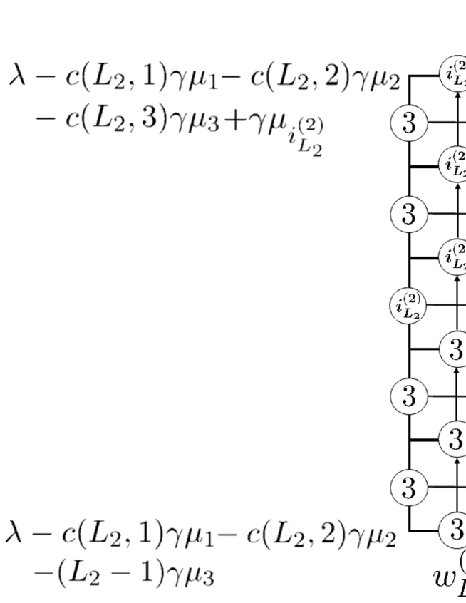
Figure 7: The states of the rightmost column of the upper region of the partition functions $W(\{{\bm{z}^{(1)}}\},\{{\bm{z}^{(2)}}\}|\{{\bm{w}^{(1)}}\},\{{\bm{w}^{(2)}}\}|\{k_{1},k_{2},L_{1},L_{2},{\bm{I}}\}|\lambda)$ giving non-zero contributions are graphically represented as above. The factors including $w_{L_{2}}^{(2)}$ all come from the dynamical $R$-matrices in this column and can be computed from the above graphical description. We get $\displaystyle h_{\ell}(w_{L_{2}}^{(2)})=[z_{\ell}^{(2)}-w_{L_{2}}^{(2)}+\lambda_{3}-\lambda_{i_{L_{2}}^{(2)}}+(c(L_{2},i_{L_{2}}^{(2)})-c(L_{2},3)-\ell)\gamma]\prod_{j=1}^{\ell-1}[z_{j}^{(2)}-w_{L_{2}}^{(2)}]\prod_{j=\ell+1}^{k_{2}}[z_{j}^{(2)}-w_{L_{2}}^{(2)}-\gamma],\ \ \ \ell=1,\cdots,k_{2}$.

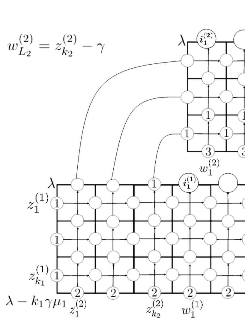
Figure 8: The partition functions of Foda-Manabe type satisfying $i_{L_{2}}^{(2)}=1$, evaluated at $w_{L_{2}}^{(2)}=z_{k_{2}}^{(2)}-\gamma$ (5.4). In the upper region, the dynamical $R$-matrices at the rightmost column and the bottom row are all frozen.

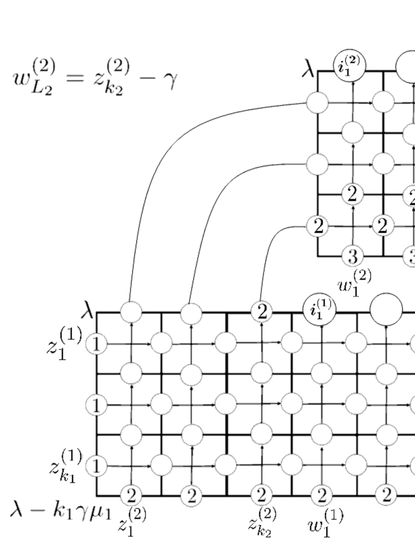
Figure 9: The partition functions of Foda-Manabe type satisfying $i_{L_{2}}^{(2)}=2$, evaluated at $w_{L_{2}}^{(2)}=z_{k_{2}}^{(2)}-\gamma$ (5.4). In the upper region, the dynamical $R$-matrices at the rightmost column and the bottom row are all frozen.

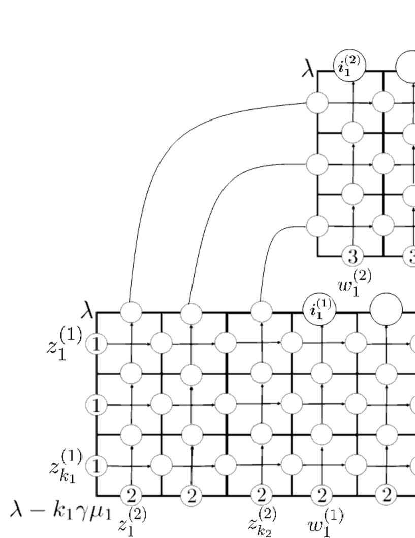
Figure 10: The partition functions of Foda-Manabe type with $i_{L_{2}}^{(2)}=3$ (5.7). The dynamical $R$-matrices at the rightmost column in the upper region are all frozen.

Proposition 5.1.

The partition functions of Foda-Manabe type associated with $E_{\tau,\eta}(gl_{3})$
$W(\{{\bm{z}^{(1)}}\},\{{\bm{z}^{(2)}}\}|\{{\bm{w}^{(1)}}\},\{{\bm{w}^{(2)}}\}|\{k_{1},k_{2},L_{1},L_{2},{\bm{I}}\}|\lambda)$ possess the following properties.

(1) When $i^{(2)}_{L_{2}}$ satisfies $i^{(2)}_{L_{2}}=1$ or $i^{(2)}_{L_{2}}=2$, the partition functions
$W(\{{\bm{z}^{(1)}}\},\{{\bm{z}^{(2)}}\}|\{{\bm{w}^{(1)}}\},\{{\bm{w}^{(2)}}\}|\{k_{1},k_{2},L_{1},L_{2},{\bm{I}}\}|\lambda)$ are elliptic polynomials of $w_{L_{2}}^{(2)}$ in $\Theta_{k_{2}}(\chi)$ with the following quasi-periodicities

$$W(\{{\bm{z}^{(1)}}\},\{{\bm{z}^{(2)}}\}|\{{\bm{w}^{(1)}}\},\{{\bm{w}^{(2)}}\}|\{k_{1},k_{2},L_{1},L_{2},{\bm{I}}\}|\lambda)|_{w^{(2)}_{L_{2}}\longrightarrow w^{(2)}_{L_{2}}+1}$$

$$= (-1)^{k_{2}}W(\{{\bm{z}^{(1)}}\},\{{\bm{z}^{(2)}}\}|\{{\bm{w}^{(1)}}\},\{{\bm{w}^{(2)}}\}|\{k_{1},k_{2},L_{1},L_{2},{\bm{I}}\}|\lambda),$$ (5.2)

$$W(\{{\bm{z}^{(1)}}\},\{{\bm{z}^{(2)}}\}|\{{\bm{w}^{(1)}}\},\{{\bm{w}^{(2)}}\}|\{k_{1},k_{2},L_{1},L_{2},{\bm{I}}\}|\lambda)|_{w^{(2)}_{L_{2}}\longrightarrow w^{(2)}_{L_{2}}+\tau}$$

$$= (-1)^{k_{2}}\mathrm{exp}\Bigg{(}-2\pi i\Bigg{(}k_{2}w_{L_{2}}^{(2)}-\sum_{i=1}^{k_{2}}z_{i}^{(2)}+\lambda_{i_{L_{2}}^{(2)}}-\lambda_{3}+\gamma(L_{2}-c(L_{2},i^{(2)}_{L_{2}}))\Bigg{)}-\pi ik_{2}\tau\Bigg{)}$$

$$\times W(\{{\bm{z}^{(1)}}\},\{{\bm{z}^{(2)}}\}|\{{\bm{w}^{(1)}}\},\{{\bm{w}^{(2)}}\}|\{k_{1},k_{2},L_{1},L_{2},{\bm{I}}\}|\lambda).$$ (5.3)

(2) The partition functions $W(\{{\bm{z}^{(1)}}\},\{{\bm{z}^{(2)}}\}|\{{\bm{w}^{(1)}}\},\{{\bm{w}^{(2)}}\}|\{k_{1},k_{2},L_{1},L_{2},{\bm{I}}\}|\lambda)$ are symmetric with respect to $z_{1}^{(2)},\dots,z_{k_{2}}^{(2)}$.

(3) If $i^{(2)}_{L_{2}}$ satisfies $i^{(2)}_{L_{2}}=1$ or $i^{(2)}_{L_{2}}=2$, the following recursive relations between the partition functions hold (Figures 8, 9):

$$W(\{{\bm{z}^{(1)}}\},\{{\bm{z}^{(2)}}\}|\{{\bm{w}^{(1)}}\},\{{\bm{w}^{(2)}}\}|\{k_{1},k_{2},L_{1},L_{2},{\bm{I}}\}|\lambda)|_{w_{L_{2}}^{(2)}=z_{k_{2}}^{(2)}-\gamma}$$

$$= \frac{[\gamma][\lambda_{3}-\lambda_{i^{(2)}_{L_{2}}}+\gamma(k_{2}-L_{2}+c(L_{2},i^{(2)}_{L_{2}}))]}{[\lambda_{i_{L_{2}}^{(2)}}-\lambda_{3}+\gamma(1-c(L_{2},i_{L_{2}}^{(2)}))]}\prod_{j=1}^{k_{2}-1}[z_{j}^{(2)}-z_{k_{2}}^{(2)}+\gamma]\prod_{j=1}^{L_{2}-1}[z_{k_{2}}^{(2)}-w_{j}^{(2)}]$$

$$\times W(\{{\bm{z}^{(1)}}\},\{{z_{1}^{(2)},\dots,z_{k_{2}-1}^{(2)}}\}|\{z_{k_{2}}^{(2)},w_{1}^{(1)},\dots,w_{L_{1}}^{(1)}\},\{w_{1}^{(2)},\dots,w_{L_{2}-1}^{(2)}\}$$

$$|\{k_{1},k_{2}-1,L_{1}+1,L_{2}-1,{\bm{J}}\}|\lambda).$$ (5.4)

Here, $W(\{{\bm{z}^{(1)}}\},\{{z_{1}^{(2)},\dots,z_{k_{2}-1}^{(2)}}\}|\{z_{k_{2}}^{(2)},w_{1}^{(1)},\dots,w_{L_{1}}^{(1)}\},\{w_{1}^{(2)},\dots,w_{L_{2}-1}^{(2)}\}|\{k_{1},k_{2}-1,L_{1}+1,L_{2}-1,{\bm{J}}\}|\lambda)$ are partition functions of size $\{k_{1},k_{2}-1,L_{1}+1,L_{2}-1\}$ whose configuration of colors are labeled by a set ${\bm{J}}:=\{{\bm{J}_{k_{1}}^{(1)}},{\bm{J}_{k_{2}-1}^{(2)}},\widehat{{\bm{J}}}_{(k_{2}-1)+(L_{1}+1)}^{(2)},\widehat{{\bm{J}}}_{L_{2}-1}^{(3)}\}$ where the subsets ${\bm{J}_{k_{1}}^{(1)}}$, ${\bm{J}_{k_{2}-1}^{(2)}}$, $\widehat{{\bm{J}}}_{(k_{2}-1)+(L_{1}+1)}^{(2)}$, $\widehat{{\bm{J}}}_{L_{2}-1}^{(3)}$ are given by ${\bm{J}_{k_{1}}^{(1)}}={\bm{I}_{k_{1}}^{(1)}}$, ${\bm{J}_{k_{2}-1}^{(2)}}={\bm{I}_{k_{2}}^{(2)}}\backslash\{L_{2}\}$, $\widehat{{\bm{J}}}_{(k_{2}-1)+(L_{1}+1)}^{(2)}=\widehat{{\bm{I}}}_{k_{2}+L_{1}}^{(2)}$, $\widehat{{\bm{J}}}_{L_{2}-1}^{(3)}=\{1,\dots,L_{2}-1\}$ satisfying the following inclusion relations

$${\bm{J}}_{k_{1}}^{(1)}\subset\widehat{{\bm{J}}}_{(k_{2}-1)+(L_{1}+1)}^{(2)}:={\bm{J}_{k_{2}-1}^{(2)}}\cup\{L_{2},\dots,L_{2}+L_{1}\},$$ (5.5)

$${\bm{J}_{k_{2}-1}^{(2)}}\subset\widehat{{\bm{J}}}_{L_{2}-1}^{(3)}:=\{1,\dots,L_{2}-1\}.$$ (5.6)

If $i^{(2)}_{L_{2}}=3$, the following factorizations hold for the partition functions (Figure 10):

$$W(\{{\bm{z}^{(1)}}\},\{{\bm{z}^{(2)}}\}|\{{\bm{w}^{(1)}}\},\{{\bm{w}^{(2)}}\}|\{k_{1},k_{2},L_{1},L_{2},{\bm{I}}\}|\lambda)$$

$$= \prod_{j=1}^{k_{2}}[z_{j}^{(2)}-w_{L_{2}}^{(2)}-\gamma]$$

$$\times W(\{{\bm{z}^{(1)}}\},\{{\bm{z}^{(2)}}\}|\{{\bm{w}^{(1)}}\},\{w_{1}^{(2)},\dots,w_{L_{2}-1}^{(2)}\}|\{k_{1},k_{2},L_{1},L_{2}-1,{\bm{K}}\}|\lambda).$$ (5.7)

Here, $W(\{{\bm{z}^{(1)}}\},\{{\bm{z}^{(2)}}\}|\{{\bm{w}^{(1)}}\},\{w_{1}^{(2)},\dots,w_{L_{2}-1}^{(2)}\}|\{k_{1},k_{2},L_{1},L_{2}-1,{\bm{K}}\}|\lambda)$ are partition functions of size $\{k_{1},k_{2},L_{1},L_{2}-1\}$ whose configuration of colors are labeled by a set ${\bm{K}}:=\{{\bm{K}_{k_{1}}^{(1)}},{\bm{K}_{k_{2}}^{(2)}},\widehat{{\bm{K}}}_{k_{2}+L_{1}}^{(2)},\widehat{{\bm{K}}}_{L_{2}-1}^{(3)}\}$ where the subsets ${\bm{K}_{k_{1}}^{(1)}}$, ${\bm{K}_{k_{2}}^{(2)}}$, $\widehat{{\bm{K}}}_{k_{2}+L_{1}}^{(2)}$, $\widehat{{\bm{K}}}_{L_{2}-1}^{(3)}$ are given by ${\bm{K}_{k_{1}}^{(1)}}={\bm{I}_{k_{1}}^{(1)}}|_{L_{2}+1\rightarrow L_{2},\dots,L_{2}+L_{1}\rightarrow L_{2}+L_{1}-1}$, ${\bm{K}_{k_{2}}^{(2)}}={\bm{I}_{k_{2}}^{(2)}}$, $\widehat{{\bm{K}}}_{k_{2}+L_{1}}^{(2)}={\bm{I}_{k_{2}}^{(2)}}\cup\{L_{2},\dots,L_{2}+L_{1}-1\}$, $\widehat{{\bm{K}}}_{L_{2}-1}^{(3)}=\{1,\dots,L_{2}-1\}$ satisfying the following inclusion relations

$${\bm{K}}_{k_{1}}^{(1)}\subset\widehat{{\bm{K}}}_{k_{2}+L_{1}}^{(2)}:={\bm{K}_{k_{2}}^{(2)}}\cup\{L_{2},\dots,L_{2}+L_{1}-1\},$$ (5.8)

$${\bm{K}_{k_{2}}^{(2)}}\subset\widehat{{\bm{K}}}_{L_{2}-1}^{(3)}:=\{1,\dots,L_{2}-1\}.$$ (5.9)

(4) When $k_{2}=1$ and $i^{(2)}_{L_{2}}$ satisfies $i^{(2)}_{L_{2}}=1$ or $i^{(2)}_{L_{2}}=2$, the following evaluation holds (Figures 11, 12) :

$$W(\{{\bm{z}^{(1)}}\},\{{\bm{z}^{(2)}}\}|\{{\bm{w}^{(1)}}\},\{{\bm{w}^{(2)}}\}|\{k_{1},1,L_{1},L_{2},{\bm{I}}\}|\lambda)$$

$$= \frac{[\gamma][z_{1}^{(2)}-w_{L_{2}}^{(2)}+\lambda_{3}-\lambda_{i_{L_{2}}^{(2)}}-\gamma(L_{2}-1)]}{[\lambda_{i_{L_{2}}^{(2)}}-\lambda_{3}]}\prod_{j=1}^{L_{2}-1}[z_{1}^{(2)}-w_{j}^{(2)}]$$

$$\times W_{L_{1}+1,k_{1}}(z_{1}^{(1)},\dots,z_{k_{1}}^{(1)}|z_{1}^{(2)},w_{1}^{(1)},\dots,w_{L_{1}}^{(1)}|I_{1}^{(1)}+1-L_{2},\dots,I_{k_{1}}^{(1)}+1-L_{2}|\lambda).$$ (5.10)

Let us give some remarks on Proposition 5.1, which corresponds to the Korepin’s lemma for the case of higher rank partition functions. An idea to anlayze partition functions which goes back to Korepin [39] is to construct relations between partition functions of different sizes. In the present case, the partition functions of type $\{k_{1},k_{2},L_{1},L_{2},{\bm{I}}\}$ is connected with other smaller partition functions (which have smaller $k_{1}+k_{2}+L_{1}+L_{2}$), and which smaller partition functions are connected depend on the color $i_{L_{2}}^{(2)}$ in the northeast corner. When $i_{L_{2}}^{(2)}=1$ or $i^{(2)}_{L_{2}}=2$, partition functions of type $\{k_{1},k_{2},L_{1},L_{2},{\bm{I}}\}$ are connected with the ones of type $\{k_{1},k_{2}-1,L_{1}+1,L_{2}-1,{\bm{J}}\}$, When $i_{L_{2}}^{(2)}=3$, the partition functions of type $\{k_{1},k_{2},L_{1},L_{2},{\bm{I}}\}$ are reduced to the ones of type $\{k_{1},k_{2},L_{1},L_{2}-1,{\bm{K}}\}$. The case $k_{2}=1$ and $i^{(2)}_{L_{2}}=1$ or $i^{(2)}_{L_{2}}=2$ correspond to the initial partition functions for this recursion, and are essentially given by the base partition functions $W_{L_{1}+1,k_{1}}(z_{1}^{(1)},\dots,z_{k_{1}}^{(1)}|z_{1}^{(2)},w_{1}^{(1)},\dots,w_{L_{1}}^{(1)}|I_{1}^{(1)}+1-L_{2},\dots,I_{k_{1}}^{(1)}+1-L_{2}|\lambda)$ which are analyzed in the previous section.

Proof.

The proof of the Izergin-Korepin analysis is basically the same with the case for the base partition functions.

Property (1) can be shown by inserting a completeness relation between the space where the spectral variable $w_{L_{2}}^{(2)}$ is associated and the space where the spectral variable $w_{L_{2}-1}^{(2)}$ is associated to split the partition functions into a sum of factors. The $w_{L_{2}}^{(2)}$-dependent factors for each summand has the following form (Figure 7):

$$h_{\ell}(w_{L_{2}}^{(2)})= [z_{\ell}^{(2)}-w_{L_{2}}^{(2)}+\lambda_{3}-\lambda_{i_{L_{2}}^{(2)}}+(c(L_{2},i_{L_{2}}^{(2)})-c(L_{2},3)-\ell)\gamma]$$

$$\times \prod_{j=1}^{\ell-1}[z_{j}^{(2)}-w_{L_{2}}^{(2)}]\prod_{j=\ell+1}^{k_{2}}[z_{j}^{(2)}-w_{L_{2}}^{(2)}-\gamma],\ \ \ \ell=1,\cdots,k_{2}.$$ (5.11)

Calculating the quasi-periodicities of $h_{\ell}(w_{L_{2}}^{(2)})$, we get

$$h_{\ell}(w_{L_{2}}^{(2)}+1) =(-1)^{k_{2}}h_{\ell}(w_{L_{2}}^{(2)}),$$ (5.12)

$$h_{\ell}(w_{L_{2}}^{(2)}+\tau) =(-1)^{k_{2}}\mathrm{exp}\Bigg{(}-2\pi i\Bigg{(}k_{2}w_{L_{2}}^{(2)}-\sum_{i=1}^{k_{2}}z_{i}^{(2)}+\lambda_{i_{L_{2}}^{(2)}}-\lambda_{3}$$

$$+\gamma(k_{2}+c(L_{2},3)-c(L_{2},i_{L_{2}}^{(2)}))\Bigg{)}-\pi ik_{2}\tau\Bigg{)}h_{\ell}(w_{L_{2}}^{(2)}),$$ (5.13)

and one finds that they are all the same for all summands, hence we get (5.2) and (5.3) (also note that $c(L_{2},3)=L_{2}-k_{2}$).

Property (2) follows from the standard railroad argument using the dynamical Yang-Baxter relation. Note that the height variables at the northwest corners in the upper region and the lower region are both fixed to $\lambda$ so that the railroad argument can be applied.

Property (3) can be shown by using the graphical representation for the partition functions. We look at the upper region where the spectral parameters $w_{1}^{(2)},\dots,w_{L_{2}}^{(2)}$ are associated. When $i^{(2)}_{L_{2}}=1$ or $i^{(2)}_{L_{2}}=2$, one can see that after the substitution $w_{L_{2}}^{(2)}=z_{k_{2}}^{(2)}-\gamma$, the dynamical $R$-matrices at the bottom row and the rightmost column in the upper region are frozen (Figures 8, 9). The product of the matrix elements of the dynamical $R$-matrices of the frozen part gives the factor

$$\frac{[\gamma][\lambda_{3}-\lambda_{i^{(2)}_{L_{2}}}+\gamma(k_{2}-L_{2}+c(L_{2},i^{(2)}_{L_{2}}))]}{[\lambda_{i_{L_{2}}^{(2)}}-\lambda_{3}+\gamma(1-c(L_{2},i_{L_{2}}^{(2)}))]}\prod_{j=1}^{k_{2}-1}[z_{j}^{(2)}-z_{k_{2}}^{(2)}+\gamma]\prod_{j=1}^{L_{2}-1}[z_{k_{2}}^{(2)}-w_{j}^{(2)}],$$ (5.14)

in the right hand side of (5.4). Next we look at the unfrozen part and we view this as a partition function of a smaller size $\{k_{1},k_{2}-1,L_{1}+1,L_{2}-1\}$. The configuration of colors are encoded into a set which we denote by ${\bm{J}}:=\{{\bm{J}_{k_{1}}^{(1)}},{\bm{J}_{k_{2}-1}^{(2)}},\widehat{{\bm{J}}}_{(k_{2}-1)+(L_{1}+1)}^{(2)},\widehat{{\bm{J}}}_{L_{2}-1}^{(3)}\}$. The set ${\bm{J}}$ is related with the set ${\bm{I}}:=\{{\bm{I}_{k_{1}}^{(1)}},{\bm{I}_{k_{2}}^{(2)}},\widehat{{\bm{I}}}_{k_{2}+L_{1}}^{(2)},\widehat{{\bm{I}}}_{L_{2}}^{(3)}\}$ for the original partition functions, and we can see from the encoding rule of the configuration of colors into sets explained in section 3 that the subsets of ${\bm{J}}$ and ${\bm{I}}$ are related by the following relations: ${\bm{J}_{k_{1}}^{(1)}}={\bm{I}_{k_{1}}^{(1)}}$, ${\bm{J}_{k_{2}-1}^{(2)}}={\bm{I}_{k_{2}}^{(2)}}\backslash\{L_{2}\}$, $\widehat{{\bm{J}}}_{(k_{2}-1)+(L_{1}+1)}^{(2)}=\widehat{{\bm{I}}}_{k_{2}+L_{1}}^{(2)}$, $\widehat{{\bm{J}}}_{L_{2}-1}^{(3)}=\{1,\dots,L_{2}-1\}$. Hence, we conclude that the original partition functions $W(\{{\bm{z}^{(1)}}\},\{{\bm{z}^{(2)}}\}|\{{\bm{w}^{(1)}}\},\{{\bm{w}^{(2)}}\}|\{k_{1},k_{2},L_{1},L_{2},{\bm{I}}\}|\lambda)$ evaluated at $w_{L_{2}}^{(2)}=z_{k_{2}}^{(2)}-\gamma$ is given by the product of the factor (5.14) and the smaller partition functions $W(\{{\bm{z}^{(1)}}\},\{{z_{1}^{(2)},\dots,z_{k_{2}-1}^{(2)}}\}|\{z_{k_{2}}^{(2)},w_{1}^{(1)},\dots,w_{L_{1}}^{(1)}\},\{w_{1}^{(2)},\dots,w_{L_{2}-1}^{(2)}\}|\{k_{1},k_{2}-1,L_{1}+1,L_{2}-1,{\bm{J}}\}|\lambda)$, i.e. we get (5.4).

We can also show (5.7) with the help of the graphical description. When $i^{(2)}_{L_{2}}=3$, one can see that the dynamical $R$-matrices at the rightmost column in the upper region are frozen (Figure 10), and the matrix elements of the dynamical $R$-matrices of this column gives the factor $\prod_{j=1}^{k_{2}}[z_{j}-w_{L_{2}}^{(2)}-\gamma]$. Peeling off the column, we get a smaller partition function of size $\{k_{1},k_{2},L_{1},L_{2}-1\}$, denoted by $W(\{{\bm{z}^{(1)}}\},\{{\bm{z}^{(2)}}\}|\{{\bm{w}^{(1)}}\},\{w_{1}^{(2)},\dots,w_{L_{2}-1}^{(2)}\}|\{k_{1},k_{2},L_{1},L_{2}-1,{\bm{K}}\}|\lambda)$. One can see that the set ${\bm{K}}:=\{{\bm{K}_{k_{1}}^{(1)}},{\bm{K}_{k_{2}}^{(2)}},\widehat{{\bm{K}}}_{k_{2}+L_{1}}^{(2)},\widehat{{\bm{K}}}_{L_{2}-1}^{(3)}\}$, which encodes the configuration of colors for the smaller partition function, is related with the set ${\bm{I}}:=\{{\bm{I}_{k_{1}}^{(1)}},{\bm{I}_{k_{2}}^{(2)}},\widehat{{\bm{I}}}_{k_{2}+L_{1}}^{(2)},\widehat{{\bm{I}}}_{L_{2}}^{(3)}\}$ for the original partition functions by the following relations: ${\bm{K}_{k_{1}}^{(1)}}={\bm{I}_{k_{1}}^{(1)}}|_{L_{2}+1\rightarrow L_{2},\dots,L_{2}+L_{1}\rightarrow L_{2}+L_{1}-1}$, ${\bm{K}_{k_{2}}^{(2)}}={\bm{I}_{k_{2}}^{(2)}}$, $\widehat{{\bm{K}}}_{k_{2}+L_{1}}^{(2)}={\bm{I}_{k_{2}}^{(2)}}\cup\{L_{2},\dots,L_{2}+L_{1}-1\}$, $\widehat{{\bm{K}}}_{L_{2}-1}^{(3)}=\{1,\dots,L_{2}-1\}$. Hence we find that the original partition functions are given by multiplying the factor $\prod_{j=1}^{k_{2}}[z_{j}-w_{L_{2}}^{(2)}-\gamma]$ by $W(\{{\bm{z}^{(1)}}\},\{{\bm{z}^{(2)}}\}|\{{\bm{w}^{(1)}}\},\{w_{1}^{(2)},\dots,w_{L_{2}-1}^{(2)}\}|\{k_{1},k_{2},L_{1},L_{2}-1,{\bm{K}}\}|\lambda)$, i.e. we get (5.7).

Property (4), which corresponds to the initial conditions of the recursion, can also be shown by graphical descriptions. When $k_{2}=1$ and $i^{(2)}_{L_{2}}=1$ or $i^{(2)}_{L_{2}}=2$, one can see that the dynamical $R$-matrices in the upper region are all frozen (Figures 11, 12), and the product of the matrix elements of the dynamical $R$-matrices gives the factor

$$\frac{[\gamma][z_{1}^{(2)}-w_{L_{2}}^{(2)}+\lambda_{3}-\lambda_{i_{L_{2}}^{(2)}}-\gamma(L_{2}-1)]}{[\lambda_{i_{L_{2}}^{(2)}}-\lambda_{3}]}\prod_{j=1}^{L_{2}-1}[z_{1}^{(2)}-w_{j}^{(2)}].$$ (5.15)

The unfrozen part is the lower region, which is nothing but the base partition function. One can see that using the elements of the set ${\bm{I}_{k_{1}}^{(1)}}=\{I_{1}^{(1)},\dots,I_{k_{1}}^{(1)}\}$ which label the configuration of colors for the original partition functions of Foda-Manabe type, the base partition function which appears as the unfrozen part is $W_{L_{1}+1,k_{1}}(z_{1}^{(1)},\dots,z_{k_{1}}^{(1)}|z_{1}^{(2)},w_{1}^{(1)},\dots,w_{L_{1}}^{(1)}|I_{1}^{(1)}+1-L_{2},\dots,I_{k_{1}}^{(1)}+1-L_{2}|\lambda).$ Hence, we find the original partition functions are given by the product of (5.15) and $W_{L_{1}+1,k_{1}}(z_{1}^{(1)},\dots,z_{k_{1}}^{(1)}|z_{1}^{(2)},w_{1}^{(1)},\dots,w_{L_{1}}^{(1)}|I_{1}^{(1)}+1-L_{2},\dots,I_{k_{1}}^{(1)}+1-L_{2}|\lambda)$ (5.10).

∎

Figure 11: The partition functions of Foda-Manabe type with $k_{2}=1$ and $i^{(2)}_{L_{2}}=1$ (5.10). One can easily see that the upper region is frozen, and the lower region is a base partition function.

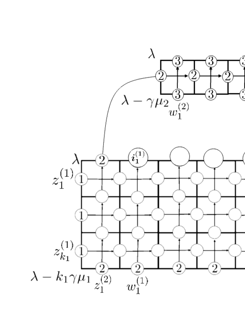
Figure 12: The partition functions of Foda-Manabe type with $k_{2}=1$ and $i^{(2)}_{L_{2}}=2$ (5.10). One can easily see that the upper region is frozen, and the lower region is a base partition function.

5.2 Elliptic multivariable functions

In this subsection, we show the elliptic multivariable functions defined below give the explicit representations for the partition functions of Foda-Manabe type by showing that they satisfy all the properties in Proposition 5.1 which $W(\{{\bm{z}^{(1)}}\},\{{\bm{z}^{(2)}}\}|\{{\bm{w}^{(1)}}\},\{{\bm{w}^{(2)}}\}|\{k_{1},k_{2},L_{1},L_{2},{\bm{I}}\}|\lambda)$ possess.

Definition 5.2.

We define the following elliptic multivariable function
$E(\{{\bm{z}^{(1)}}\},\{{\bm{z}^{(2)}}\}|\{{\bm{w}^{(1)}}\},\{{\bm{w}^{(2)}}\}|\{k_{1},k_{2},L_{1},L_{2},{\bm{I}}\}|\lambda)$ which depend on two sets of symmetric variables $\{{\bm{z}^{(1)}}\}$, $\{{\bm{z}^{(2)}}\}$, two sets of complex parameters $\{{\bm{w}^{(1)}}\}$, $\{{\bm{w}^{(2)}}\}$, complex parameters $\gamma$, $\lambda_{1}$, $\lambda_{2}$, $\lambda_{3}$ and a set $\{k_{1},k_{2},L_{1},L_{2},{\bm{I}}\}$, ${\bm{I}}=\{{\bm{I}_{k_{1}}^{(1)}},{\bm{I}_{k_{2}}^{(2)}},\widehat{{\bm{I}}}_{k_{2}+L_{1}}^{(2)},\widehat{{\bm{I}}}_{L_{2}}^{(3)}\}$ which is equivalent to “the configuration of colors” $i_{1}^{(1)},\dots,\dots,i_{L_{1}}^{(1)}\in\{1,2\}$, $i_{1}^{(2)},\dots,\dots,i_{L_{2}}^{(2)}\in\{1,2,3\}$,

$$E(\{{\bm{z}^{(1)}}\},\{{\bm{z}^{(2)}}\}|\{{\bm{w}^{(1)}}\},\{{\bm{w}^{(2)}}\}|\{k_{1},k_{2},L_{1},L_{2},{\bm{I}}\}|\lambda)$$

$$= [\gamma]^{k_{1}+k_{2}}\sum_{\sigma_{1}\in S_{k_{1}}}\sum_{\sigma_{2}\in S_{k_{2}}}\prod_{a=1}^{k_{1}}\Bigg{(}\prod_{i=1}^{\widetilde{I_{a}^{(1)}}-1}[z_{\sigma_{1}(a)}^{(1)}-m_{i}^{k_{2},L_{1}}(\{{\bm{z}_{\sigma_{2}}^{(2)}}\}|\{{\bm{w}^{(1)}}\})]$$

$$\times \frac{[z_{\sigma_{1}(a)}^{(1)}-m_{\widetilde{I_{a}^{(1)}}}^{k_{2},L_{1}}(\{{\bm{z}_{\sigma_{2}}^{(2)}}\}|\{{\bm{w}^{(1)}}\})+\lambda_{2}-\lambda_{1}+\gamma(2a-1-\widetilde{I_{a}^{(1)}})]}{[\lambda_{1}-\lambda_{2}+(1-a)\gamma]}$$

$$\times \prod_{i={\widetilde{I_{a}^{(1)}}+1}}^{k_{2}+L_{1}}[z_{\sigma_{1}(a)}^{(1)}-m_{i}^{k_{2},L_{1}}(\{{\bm{z}_{\sigma_{2}}^{(2)}}\}|\{{\bm{w}^{(1)}}\})-\gamma]\Bigg{)}$$

$$\times \prod_{1\leq a<b\leq k_{1}}\frac{[z_{\sigma_{1}(a)}^{(1)}-z_{\sigma_{1}(b)}^{(1)}+\gamma]}{[z_{\sigma_{1}(a)}^{(1)}-z_{\sigma_{1}(b)}^{(1)}]}\prod_{a=1}^{k_{2}}\Bigg{(}\prod_{i=1}^{I_{a}^{(2)}-1}[z_{\sigma_{2}(a)}^{(2)}-w_{i}^{(2)}]$$

$$\times \frac{[z_{\sigma_{2}(a)}^{(2)}-w_{I_{a}^{(2)}}^{(2)}+\lambda_{3}-\lambda_{i_{I_{a}^{(2)}}^{(2)}}+(a-I_{a}^{(2)}-1+c(I_{a}^{(2)},i_{I_{a}^{(2)}}^{(2)}))\gamma]}{[\lambda_{i_{I_{a}^{(2)}}^{(2)}}-\lambda_{3}+(1-c(I_{a}^{(2)},i_{I_{a}^{(2)}}^{(2)}))\gamma]}$$

$$\times \prod_{i=I_{a}^{(2)}+1}^{L_{2}}[z_{\sigma_{2}(a)}^{(2)}-w_{i}^{(2)}-\gamma]\Bigg{)}\prod_{1\leq a<b\leq k_{2}}\frac{[z_{\sigma_{2}(a)}^{(2)}-z_{\sigma_{2}(b)}^{(2)}+\gamma]}{[z_{\sigma_{2}(a)}^{(2)}-z_{\sigma_{2}(b)}^{(2)}]},$$ (5.16)

where $m_{i}^{k_{2},L_{1}}(\{{\bm{z}^{(2)}}\}|\{{\bm{w}^{(1)}}\})$ and $c(k,j)$ are given by

$$m_{i}^{k_{2},L_{1}}(\{{\bm{z}^{(2)}}\}|\{{\bm{w}^{(1)}}\})=\begin{cases}z_{i}^{(2)}&1\leq i\leq k_{2}\\ w_{i-k_{2}}^{(1)}&k_{2}+1\leq i\leq k_{2}+L_{1}\end{cases},$$ (5.17)

and

$$c(k,j)=\#\{\ell|1\leq\ell\leq k,i_{\ell}^{(2)}=j\}.$$ (5.18)

The relation between the Foda-Manabe label $\{k_{1},k_{2},L_{1},L_{2},{\bm{I}}\}$, ${\bm{I}}=\{{\bm{I}_{k_{1}}^{(1)}},{\bm{I}_{k_{2}}^{(2)}},\widehat{{\bm{I}}}_{k_{2}+L_{1}}^{(2)},\widehat{{\bm{I}}}_{L_{2}}^{(3)}\}$ and “the configuration of colors” $i_{1}^{(1)},\dots,\dots,i_{L_{1}}^{(1)}\in\{1,2\}$, $i_{1}^{(2)},\dots,\dots,i_{L_{2}}^{(2)}\in\{1,2,3\}$, and the induced label $\widetilde{{\bm{I}_{k_{1}}^{(1)}}}$ which is induced from the map $\displaystyle{\bm{I}}_{k_{1}}^{(1)}\subset\widehat{{\bm{I}}}_{k_{2}+L_{1}}^{(2)}\longrightarrow\widetilde{{\bm{I}_{k_{1}}^{(1)}}}\subset\{1,\dots,k_{2}+L_{1}\}$, are explained in section 3.

Theorem 5.3.

The partition functions $W(\{{\bm{z}^{(1)}}\},\{{\bm{z}^{(2)}}\}|\{{\bm{w}^{(1)}}\},\{{\bm{w}^{(2)}}\}|\{k_{1},k_{2},L_{1},L_{2},{\bm{I}}\}|\lambda)$ of Foda-Manabe type associated with $E_{\tau,\gamma}(gl_{3})$ are explicitly expressed as the multivariable elliptic symmetric functions $E(\{{\bm{z}^{(1)}}\},\{{\bm{z}^{(2)}}\}|\{{\bm{w}^{(1)}}\},\{{\bm{w}^{(2)}}\}|\{k_{1},k_{2},L_{1},L_{2},{\bm{I}}\}|\lambda)$,

$$W(\{{\bm{z}^{(1)}}\},\{{\bm{z}^{(2)}}\}|\{{\bm{w}^{(1)}}\},\{{\bm{w}^{(2)}}\}|\{k_{1},k_{2},L_{1},L_{2},{\bm{I}}\}|\lambda)$$

$$= E(\{{\bm{z}^{(1)}}\},\{{\bm{z}^{(2)}}\}|\{{\bm{w}^{(1)}}\},\{{\bm{w}^{(2)}}\}|\{k_{1},k_{2},L_{1},L_{2},{\bm{I}}\}|\lambda).$$ (5.19)

Proof.

We show that the functions $E(\{{\bm{z}^{(1)}}\},\{{\bm{z}^{(2)}}\}|\{{\bm{w}^{(1)}}\},\{{\bm{w}^{(2)}}\}|\{k_{1},k_{2},L_{1},L_{2},{\bm{I}}\}|\lambda)$ satisfy all the properties in Proposition 5.1 which the partition functions of Foda-Manabe type $W(\{{\bm{z}^{(1)}}\},\{{\bm{z}^{(2)}}\}|\{{\bm{w}^{(1)}}\},\{{\bm{w}^{(2)}}\}|\{k_{1},k_{2},L_{1},L_{2},{\bm{I}}\}|\lambda)$ satisfy.

Properties (2) and (4) are easy to check from the definition of the elliptic multivariable functions $E(\{{\bm{z}^{(1)}}\},\{{\bm{z}^{(2)}}\}|\{{\bm{w}^{(1)}}\},\{{\bm{w}^{(2)}}\}|\{k_{1},k_{2},L_{1},L_{2},{\bm{I}}\}|\lambda)$ (5.16).

Let us show Property (1) and (5.4) in Property (3). When $i_{L_{2}}^{(2)}=1$ or $i_{L_{2}}^{(2)}=2$, we note $I_{k_{2}}^{(2)}=L_{2}$ since $L_{2}\in{\bm{I}_{k_{2}}^{(2)}}$. From this fact, one finds that each summand in (5.16) contains the following product of factors

$$f_{\sigma_{2}}(w_{L_{2}}^{(2)})$$

$$=[z_{\sigma_{2}(k_{2})}^{(2)}-w_{L_{2}}^{(2)}+\lambda_{3}-\lambda_{i_{L_{2}}^{(2)}}+\gamma(k_{2}-L_{2}-1+c(L_{2},i_{L_{2}}^{(2)}))]\prod_{a=1}^{k_{2}-1}[z_{\sigma_{2}(a)}^{(2)}-w_{L_{2}}^{(2)}-\gamma],$$ (5.20)

from which all the $w_{L_{2}}^{(2)}$-dependence comes. One can easily compute the quasi-periodicities for $f_{\sigma_{2}}(w_{L_{2}}^{(2)})$

$$f_{\sigma_{2}}(w_{L_{2}}^{(2)}+1)=(-1)^{k_{2}}f_{\sigma_{2}}(w_{L_{2}}^{(2)}),$$

$$f_{\sigma_{2}}(w_{L_{2}}^{(2)}+\tau)$$

$$= (-1)^{k_{2}}\mathrm{exp}\Bigg{(}-2\pi i\Bigg{(}k_{2}w_{L_{2}}^{(2)}-\sum_{i=1}^{k_{2}}z_{i}^{(2)}+\lambda_{i_{L_{2}}^{(2)}}-\lambda_{3}+\gamma(L_{2}-c(L_{2},i^{(2)}_{L_{2}}))\Bigg{)}-\pi ik_{2}\tau\Bigg{)}f_{\sigma_{2}}(w_{L_{2}}^{(2)}).$$

We find the quasi-periodicities are independent of $\sigma_{2}$, and from this explicit expression, one concludes that the elliptic multivariable functions satisfy the same quasi-periodicities with the partition functions (5.2) and (5.3).

We continue the argument to show (5.4). We note from the factor (5.20) for each summand in $E(\{{\bm{z}^{(1)}}\},\{{\bm{z}^{(2)}}\}|\{{\bm{w}^{(1)}}\},\{{\bm{w}^{(2)}}\}|\{k_{1},k_{2},L_{1},L_{2},{\bm{I}}\}|\lambda)$ that only the summands satisfying $\sigma_{2}(k_{2})=k_{2}$ in (5.16) survive after the substitution $w_{L_{2}}^{(2)}=z_{k_{2}}^{(2)}-\gamma$. Then we find that after the substitution $w_{L_{2}}^{(2)}=z_{k_{2}}^{(2)}-\gamma$, the following product of factors

$$[\gamma]^{k_{1}+k_{2}}$$

$$\times \prod_{a=1}^{k_{2}}\Bigg{(}\prod_{i=1}^{I_{a}^{(2)}-1}[z_{\sigma_{2}(a)}^{(2)}-w_{i}^{(2)}]\frac{[z_{\sigma_{2}(a)}^{(2)}-w_{I_{a}^{(2)}}^{(2)}+\lambda_{3}-\lambda_{i_{I_{a}^{(2)}}^{(2)}}+(a-I_{a}^{(2)}-1+c(I_{a}^{(2)},i_{I_{a}^{(2)}}^{(2)}))\gamma]}{[\lambda_{i_{I_{a}^{(2)}}^{(2)}}-\lambda_{3}+(1-c(I_{a}^{(2)},i_{I_{a}^{(2)}}^{(2)}))\gamma]}$$

$$\times \prod_{i=I_{a}^{(2)}+1}^{L_{2}}[z_{\sigma_{2}(a)}^{(2)}-w_{i}^{(2)}-\gamma]\Bigg{)}\prod_{1\leq a<b\leq k_{2}}\frac{[z_{\sigma_{2}(a)}^{(2)}-z_{\sigma_{2}(b)}^{(2)}+\gamma]}{[z_{\sigma_{2}(a)}^{(2)}-z_{\sigma_{2}(b)}^{(2)}]},$$ (5.21)

in each summand in (5.16) can be rewritten as

$$[\gamma]^{k_{1}+k_{2}-1}$$

$$\times \prod_{a=1}^{k_{2}-1}\Bigg{(}\prod_{i=1}^{I_{a}^{(2)}-1}[z_{\sigma_{2}(a)}^{(2)}-w_{i}^{(2)}]\frac{[z_{\sigma_{2}(a)}^{(2)}-w_{I_{a}^{(2)}}^{(2)}+\lambda_{3}-\lambda_{i_{I_{a}^{(2)}}^{(2)}}+(a-I_{a}^{(2)}-1+c(I_{a}^{(2)},i_{I_{a}^{(2)}}^{(2)}))\gamma]}{[\lambda_{i_{I_{a}^{(2)}}^{(2)}}-\lambda_{3}+(1-c(I_{a}^{(2)},i_{I_{a}^{(2)}}^{(2)}))\gamma]}$$

$$\times \prod_{i=I_{a}^{(2)}+1}^{L_{2}-1}[z_{\sigma_{2}(a)}^{(2)}-w_{i}^{(2)}-\gamma]\Bigg{)}\prod_{1\leq a<b\leq k_{2}-1}\frac{[z_{\sigma_{2}(a)}^{(2)}-z_{\sigma_{2}(b)}^{(2)}+\gamma]}{[z_{\sigma_{2}(a)}^{(2)}-z_{\sigma_{2}(b)}^{(2)}]}$$

$$\times \frac{[\gamma][\lambda_{3}-\lambda_{i^{(2)}_{L_{2}}}+\gamma(k_{2}-L_{2}+c(L_{2},i^{(2)}_{L_{2}}))]}{[\lambda_{i_{L_{2}}^{(2)}}-\lambda_{3}+\gamma(1-c(L_{2},i_{L_{2}}^{(2)}))]}\prod_{j=1}^{k_{2}-1}[z_{j}^{(2)}-z_{k_{2}}^{(2)}+\gamma]\prod_{j=1}^{L_{2}-1}[z_{k_{2}}^{(2)}-w_{j}^{(2)}].$$ (5.22)

We further rewrite this using the set ${\bm{J}}=\{{\bm{J}_{k_{1}}^{(1)}},{\bm{J}_{k_{2}-1}^{(2)}},\widehat{{\bm{J}}}_{(k_{2}-1)+(L_{1}+1)}^{(2)},\widehat{{\bm{J}}}_{L_{2}-1}^{(3)}\}$ whose relation with the set ${\bm{I}}=\{{\bm{I}_{k_{1}}^{(1)}},{\bm{I}_{k_{2}}^{(2)}},\widehat{{\bm{I}}}_{k_{2}+L_{1}}^{(2)},\widehat{{\bm{I}}}_{L_{2}}^{(3)}\}$ is given in Proposition 5.1. Since ${\bm{J}_{k_{2}-1}^{(2)}}={\bm{I}_{k_{2}}^{(2)}}\backslash\{L_{2}\}$ and $I_{k_{2}}^{(2)}=L_{2}$, we have the following relation $J_{a}^{(2)}=I_{a}^{(2)}$, $a=1,\dots,k_{2}-1$. Using this relation, (5.22) can be rewritten as

$$[\gamma]^{k_{1}+k_{2}-1}$$

$$\times \prod_{a=1}^{k_{2}-1}\Bigg{(}\prod_{i=1}^{J_{a}^{(2)}-1}[z_{\sigma_{2}(a)}^{(2)}-w_{i}^{(2)}]\frac{[z_{\sigma_{2}(a)}^{(2)}-w_{J_{a}^{(2)}}^{(2)}+\lambda_{3}-\lambda_{i_{J_{a}^{(2)}}^{(2)}}+(a-J_{a}^{(2)}-1+c(J_{a}^{(2)},i_{J_{a}^{(2)}}^{(2)}))\gamma]}{[\lambda_{i_{J_{a}^{(2)}}^{(2)}}-\lambda_{3}+(1-c(J_{a}^{(2)},i_{J_{a}^{(2)}}^{(2)}))\gamma]}$$

$$\times \prod_{i=J_{a}^{(2)}+1}^{L_{2}-1}[z_{\sigma_{2}(a)}^{(2)}-w_{i}^{(2)}-\gamma]\Bigg{)}\prod_{1\leq a<b\leq k_{2}-1}\frac{[z_{\sigma_{2}(a)}^{(2)}-z_{\sigma_{2}(b)}^{(2)}+\gamma]}{[z_{\sigma_{2}(a)}^{(2)}-z_{\sigma_{2}(b)}^{(2)}]}$$

$$\times \frac{[\gamma][\lambda_{3}-\lambda_{i^{(2)}_{L_{2}}}+\gamma(k_{2}-L_{2}+c(L_{2},i^{(2)}_{L_{2}}))]}{[\lambda_{i_{L_{2}}^{(2)}}-\lambda_{3}+\gamma(1-c(L_{2},i_{L_{2}}^{(2)}))]}\prod_{j=1}^{k_{2}-1}[z_{j}^{(2)}-z_{k_{2}}^{(2)}+\gamma]\prod_{j=1}^{L_{2}-1}[z_{k_{2}}^{(2)}-w_{j}^{(2)}].$$ (5.23)

We next rewrite the remaining product of factors

$$\prod_{a=1}^{k_{1}}\Bigg{(}\prod_{i=1}^{\widetilde{I_{a}^{(1)}}-1}[z_{\sigma_{1}(a)}^{(1)}-m_{i}^{k_{2},L_{1}}(\{{\bm{z}_{\sigma_{2}}^{(2)}}\}|\{{\bm{w}^{(1)}}\})]$$

$$\times \frac{[z_{\sigma_{1}(a)}^{(1)}-m_{\widetilde{I_{a}^{(1)}}}^{k_{2},L_{1}}(\{{\bm{z}_{\sigma_{2}}^{(2)}}\}|\{{\bm{w}^{(1)}}\})+\lambda_{2}-\lambda_{1}+\gamma(2a-1-\widetilde{I_{a}^{(1)}})]}{[\lambda_{1}-\lambda_{2}+(1-a)\gamma]}$$

$$\times \prod_{i={\widetilde{I_{a}^{(1)}}+1}}^{k_{2}+L_{1}}[z_{\sigma_{1}(a)}^{(1)}-m_{i}^{k_{2},L_{1}}(\{{\bm{z}_{\sigma_{2}}^{(2)}}\}|\{{\bm{w}^{(1)}}\})-\gamma]\Bigg{)}\prod_{1\leq a<b\leq k_{1}}\frac{[z_{\sigma_{1}(a)}^{(1)}-z_{\sigma_{1}(b)}^{(1)}+\gamma]}{[z_{\sigma_{1}(a)}^{(1)}-z_{\sigma_{1}(b)}^{(1)}]},$$ (5.24)

which, together with the factors (5.21), forms each summand in (5.16). We again rewrite using the set ${\bm{J}}=\{{\bm{J}_{k_{1}}^{(1)}},{\bm{J}_{k_{2}-1}^{(2)}},\widehat{{\bm{J}}}_{(k_{2}-1)+(L_{1}+1)}^{(2)},\widehat{{\bm{J}}}_{L_{2}-1}^{(3)}\}$.

First, let us recall that only the summands satisfying $\sigma_{2}(k_{2})=k_{2}$ in (5.16) survive after the substitution $w_{L_{2}}^{(2)}=z_{k_{2}}^{(2)}-\gamma$. When $\sigma_{2}(k_{2})=k_{2}$, we can rewrite $m_{i}^{k_{2},L_{1}}(\{{\bm{z}_{\sigma_{2}}^{(2)}}\}|\{{\bm{w}^{(1)}}\})$ as

$$m_{i}^{k_{2},L_{1}}(\{{\bm{z}_{\sigma_{2}}^{(2)}}\}|\{{\bm{w}^{(1)}}\})=\begin{cases}z_{\sigma_{2}(i)}^{(2)}&1\leq i\leq k_{2}-1\\ z_{k_{2}}^{(2)}&i=k_{2}\\ w_{i-k_{2}}^{(1)}&k_{2}+1\leq i\leq k_{2}+L_{1}\end{cases}$$

$$= m_{i}^{k_{2}-1,L_{1}+1}(\{z_{\sigma_{2}(1)}^{(2)},\dots,z_{\sigma_{2}(k_{2}-1)}^{(2)}\}|\{z_{k_{2}}^{(2)},w_{1}^{(1)},\dots,w_{L_{1}}^{(1)}\}),$$ (5.25)

which can be easily checked from the definition of $m_{i}^{k_{2},L_{1}}(\{{\bm{z}^{(2)}}\}|\{{\bm{w}^{(1)}}\})$ (5.17).

We also note that since ${\bm{J}_{k_{1}}^{(1)}}={\bm{I}_{k_{1}}^{(1)}}$ and $\widehat{{\bm{J}}}_{(k_{2}-1)+(L_{1}+1)}^{(2)}=\widehat{{\bm{I}}}_{k_{2}+L_{1}}^{(2)}$, the inclusion relation ${\bm{J}}_{k_{1}}^{(1)}\subset\widehat{{\bm{J}}}_{(k_{2}-1)+(L_{1}+1)}^{(2)}$ for ${\bm{J}}$ is exactly the same with the one ${\bm{I}}_{k_{1}}^{(1)}\subset\widehat{{\bm{I}}}_{k_{2}+L_{1}}^{(2)}$ for ${\bm{I}}$. The induced sets $\widetilde{{\bm{J}_{k_{1}}^{(1)}}}$ and $\widetilde{{\bm{I}_{k_{1}}^{(1)}}}$ are induced from these inclusion relations in the same way and since both relations are exactly the same, we conclude $\widetilde{{\bm{J}_{k_{1}}^{(1)}}}=\widetilde{{\bm{I}_{k_{1}}^{(1)}}}$. Hence the elements of both sets are all the same $\widetilde{J_{a}^{(1)}}=\widetilde{I_{a}^{(1)}}$, $a=1,\dots,k_{1}$ and one can rewrite (5.24) using the set ${\bm{J}}=\{{\bm{J}_{k_{1}}^{(1)}},{\bm{J}_{k_{2}-1}^{(2)}},\widehat{{\bm{J}}}_{(k_{2}-1)+(L_{1}+1)}^{(2)},\widehat{{\bm{J}}}_{L_{2}-1}^{(3)}\}$ as

$$\prod_{a=1}^{k_{1}}\Bigg{(}\prod_{i=1}^{\widetilde{J_{a}^{(1)}}-1}[z_{\sigma_{1}(a)}^{(1)}-m_{i}^{k_{2}-1,L_{1}+1}(\{z_{\sigma_{2}(1)}^{(2)},\dots,z_{\sigma_{2}(k_{2}-1)}^{(2)}\}|\{z_{k_{2}}^{(2)},w_{1}^{(1)},\dots,w_{L_{1}}^{(1)}\})]$$

$$\times \frac{[z_{\sigma_{1}(a)}^{(1)}-m_{\widetilde{J_{a}^{(1)}}}^{k_{2}-1,L_{1}+1}(\{z_{\sigma_{2}(1)}^{(2)},\dots,z_{\sigma_{2}(k_{2}-1)}^{(2)}\}|\{z_{k_{2}}^{(2)},w_{1}^{(1)},\dots,w_{L_{1}}^{(1)}\})+\lambda_{2}-\lambda_{1}+\gamma(2a-1-\widetilde{J_{a}^{(1)}})]}{[\lambda_{1}-\lambda_{2}+(1-a)\gamma]}$$

$$\times \prod_{i={\widetilde{J_{a}^{(1)}}+1}}^{(k_{2}-1)+(L_{1}+1)}[z_{\sigma_{1}(a)}^{(1)}-m_{i}^{k_{2}-1,L_{1}+1}(\{z_{\sigma_{2}(1)}^{(2)},\dots,z_{\sigma_{2}(k_{2}-1)}^{(2)}\}|\{z_{k_{2}}^{(2)},w_{1}^{(1)},\dots,w_{L_{1}}^{(1)}\})-\gamma]\Bigg{)}$$

$$\times \prod_{1\leq a<b\leq k_{1}}\frac{[z_{\sigma_{1}(a)}^{(1)}-z_{\sigma_{1}(b)}^{(1)}+\gamma]}{[z_{\sigma_{1}(a)}^{(1)}-z_{\sigma_{1}(b)}^{(1)}]}.$$ (5.26)

Combining the two factors (5.23) and (5.26) whose product gives each summand in the elliptic multivariable functions, we find that $E(\{{\bm{z}^{(1)}}\},\{{\bm{z}^{(2)}}\}|\{{\bm{w}^{(1)}}\},\{{\bm{w}^{(2)}}\}|\{k_{1},k_{2},L_{1},L_{2},{\bm{I}}\}|\lambda)$ evaluated at $w_{L_{2}}^{(2)}=z_{k_{2}}^{(2)}-\gamma$ can be expressed as

$$E(\{{\bm{z}^{(1)}}\},\{{\bm{z}^{(2)}}\}|\{{\bm{w}^{(1)}}\},\{{\bm{w}^{(2)}}\}|\{k_{1},k_{2},L_{1},L_{2},{\bm{I}}\}|\lambda)|_{w_{L_{2}}^{(2)}=z_{k_{2}}^{(2)}-\gamma}$$

$$= [\gamma]^{k_{1}+k_{2}-1}\sum_{\sigma_{1}\in S_{k_{1}}}\sum_{\sigma_{2}\in S_{k_{2}-1}}$$

$$\times \prod_{a=1}^{k_{1}}\Bigg{(}\prod_{i=1}^{\widetilde{J_{a}^{(1)}}-1}[z_{\sigma_{1}(a)}^{(1)}-m_{i}^{k_{2}-1,L_{1}+1}(\{z_{\sigma_{2}(1)}^{(2)},\dots,z_{\sigma_{2}(k_{2}-1)}^{(2)}\}|\{z_{k_{2}}^{(2)},w_{1}^{(1)},\dots,w_{L_{1}}^{(1)}\})]$$

$$\times \frac{[z_{\sigma_{1}(a)}^{(1)}-m_{\widetilde{J_{a}^{(1)}}}^{k_{2}-1,L_{1}+1}(\{z_{\sigma_{2}(1)}^{(2)},\dots,z_{\sigma_{2}(k_{2}-1)}^{(2)}\}|\{z_{k_{2}}^{(2)},w_{1}^{(1)},\dots,w_{L_{1}}^{(1)}\})+\lambda_{2}-\lambda_{1}+\gamma(2a-1-\widetilde{J_{a}^{(1)}})]}{[\lambda_{1}-\lambda_{2}+(1-a)\gamma]}$$

$$\times \prod_{i={\widetilde{J_{a}^{(1)}}+1}}^{(k_{2}-1)+(L_{1}+1)}[z_{\sigma_{1}(a)}^{(1)}-m_{i}^{k_{2}-1,L_{1}+1}(\{z_{\sigma_{2}(1)}^{(2)},\dots,z_{\sigma_{2}(k_{2}-1)}^{(2)}\}|\{z_{k_{2}}^{(2)},w_{1}^{(1)},\dots,w_{L_{1}}^{(1)}\})-\gamma]\Bigg{)}$$

$$\times \prod_{1\leq a<b\leq k_{1}}\frac{[z_{\sigma_{1}(a)}^{(1)}-z_{\sigma_{1}(b)}^{(1)}+\gamma]}{[z_{\sigma_{1}(a)}^{(1)}-z_{\sigma_{1}(b)}^{(1)}]}$$

$$\times \prod_{a=1}^{k_{2}-1}\Bigg{(}\prod_{i=1}^{J_{a}^{(2)}-1}[z_{\sigma_{2}(a)}^{(2)}-w_{i}^{(2)}]\frac{[z_{\sigma_{2}(a)}^{(2)}-w_{J_{a}^{(2)}}^{(2)}+\lambda_{3}-\lambda_{i_{J_{a}^{(2)}}^{(2)}}+(a-J_{a}^{(2)}-1+c(J_{a}^{(2)},i_{J_{a}^{(2)}}^{(2)}))\gamma]}{[\lambda_{i_{J_{a}^{(2)}}^{(2)}}-\lambda_{3}+(1-c(J_{a}^{(2)},i_{J_{a}^{(2)}}^{(2)}))\gamma]}$$

$$\times \prod_{i=J_{a}^{(2)}+1}^{L_{2}-1}[z_{\sigma_{2}(a)}^{(2)}-w_{i}^{(2)}-\gamma]\Bigg{)}\prod_{1\leq a<b\leq k_{2}-1}\frac{[z_{\sigma_{2}(a)}^{(2)}-z_{\sigma_{2}(b)}^{(2)}+\gamma]}{[z_{\sigma_{2}(a)}^{(2)}-z_{\sigma_{2}(b)}^{(2)}]}$$

$$\times \frac{[\gamma][\lambda_{3}-\lambda_{i^{(2)}_{L_{2}}}+\gamma(k_{2}-L_{2}+c(L_{2},i^{(2)}_{L_{2}}))]}{[\lambda_{i_{L_{2}}^{(2)}}-\lambda_{3}+\gamma(1-c(L_{2},i_{L_{2}}^{(2)}))]}\prod_{j=1}^{k_{2}-1}[z_{j}^{(2)}-z_{k_{2}}^{(2)}+\gamma]\prod_{j=1}^{L_{2}-1}[z_{k_{2}}^{(2)}-w_{j}^{(2)}]$$

$$= \frac{[\gamma][\lambda_{3}-\lambda_{i^{(2)}_{L_{2}}}+\gamma(k_{2}-L_{2}+c(L_{2},i^{(2)}_{L_{2}}))]}{[\lambda_{i_{L_{2}}^{(2)}}-\lambda_{3}+\gamma(1-c(L_{2},i_{L_{2}}^{(2)}))]}\prod_{j=1}^{k_{2}-1}[z_{j}^{(2)}-z_{k_{2}}^{(2)}+\gamma]\prod_{j=1}^{L_{2}-1}[z_{k_{2}}^{(2)}-w_{j}^{(2)}]$$

$$\times E(\{{\bm{z}^{(1)}}\},\{{z_{1}^{(2)},\dots,z_{k_{2}-1}^{(2)}}\}|\{z_{k_{2}}^{(2)},w_{1}^{(1)},\dots,w_{L_{1}}^{(1)}\},\{w_{1}^{(2)},\dots,w_{L_{2}-1}^{(2)}\}$$

$$|\{k_{1},k_{2}-1,L_{1}+1,L_{2}-1,{\bm{J}}\}|\lambda).$$ (5.27)

This relation for the elliptic functions is exactly the same as the relation (5.4) for the partition functions $W(\{{\bm{z}^{(1)}}\},\{{\bm{z}^{(2)}}\}|\{{\bm{w}^{(1)}}\},\{{\bm{w}^{(2)}}\}|\{k_{1},k_{2},L_{1},L_{2},{\bm{I}}\}|\lambda)$, and hence property (3) for the case $i_{L_{2}}^{(2)}=1$ or $i_{L_{2}}^{(2)}=2$ is shown.

Let us show the case when $i_{L_{2}}^{(2)}=3$ which can be shown in a similar way. We rewrite the elliptic functions using the set ${\bm{K}}=\{{\bm{K}_{k_{1}}^{(1)}},{\bm{K}_{k_{2}}^{(2)}},\widehat{{\bm{K}}}_{k_{2}+L_{1}}^{(2)},\widehat{{\bm{K}}}_{L_{2}-1}^{(3)}\}$, whose relation with ${\bm{I}}:=\{{\bm{I}_{k_{1}}^{(1)}},{\bm{I}_{k_{2}}^{(2)}},\widehat{{\bm{I}}}_{k_{2}+L_{1}}^{(2)},\widehat{{\bm{I}}}_{L_{2}}^{(3)}\}$ is given in Proposition 5.1.

First, we note $K_{a}^{(2)}=I_{a}^{(2)}$, $a=1,\dots,k_{2}$ since ${\bm{K}_{k_{2}}^{(2)}}={\bm{I}_{k_{2}}^{(2)}}$. Next, using ${\bm{K}}_{k_{1}}^{(1)}={\bm{I}}_{k_{1}}^{(1)}|_{L_{2}+1\rightarrow L_{2},\dots,L_{2}+L_{1}\rightarrow L_{2}+L_{1}-1}$ and $\widehat{{\bm{K}}}_{k_{2}+L_{1}}^{(2)}={\bm{K}_{k_{2}}^{(2)}}\cup\{L_{2},\dots,L_{2}+L_{1}-1\}={\bm{I}_{k_{2}}^{(2)}}\cup\{L_{2},\dots,L_{2}+L_{1}-1\}={\bm{I}_{k_{2}}^{(2)}}\cup\{L_{2}+1,\dots,L_{2}+L_{1}\}|_{L_{2}+1\rightarrow L_{2},\dots,L_{2}+L_{1}\rightarrow L_{2}+L_{1}-1}=\widehat{{\bm{I}}}_{k_{2}+L_{1}}^{(2)}|_{L_{2}+1\rightarrow L_{2},\dots,L_{2}+L_{1}\rightarrow L_{2}+L_{1}-1}$, one finds that the inclusion relation ${\bm{K}}_{k_{1}}^{(1)}\subset\widehat{{\bm{K}}}_{k_{2}+L_{1}}^{(2)}:={\bm{K}_{k_{2}}^{(2)}}\cup\{L_{2},\dots,L_{2}+L_{1}-1\}$ can be rewritten as ${\bm{I}}_{k_{1}}^{(1)}|_{L_{2}+1\rightarrow L_{2},\dots,L_{2}+L_{1}\rightarrow L_{2}+L_{1}-1}\subset\widehat{{\bm{I}}}_{k_{2}+L_{1}}^{(2)}|_{L_{2}+1\rightarrow L_{2},\dots,L_{2}+L_{1}\rightarrow L_{2}+L_{1}-1}$. From this rewriting, we find that the induced sets induced by the mapping the inclusion relations to $\{1,\dots,k_{2}+L_{1}\}$ are exactly the same $\widetilde{{\bm{K}_{k_{1}}^{(1)}}}=\widetilde{{\bm{I}_{k_{1}}^{(1)}}}$, hence we get $\widetilde{K_{a}^{(1)}}=\widetilde{I_{a}^{(1)}}$, $a=1,\dots,k_{1}$. Finally, note that when $i_{L_{2}}^{(2)}=3$, $I_{k_{2}}^{(2)}\leq L_{2}-1$ holds since $L_{2}\notin{\bm{I}_{k_{2}}^{(2)}}$, and using this fact, one rewrites the factor $\displaystyle\prod_{a=1}^{k_{2}}\prod_{i=I_{a}^{(2)}+1}^{L_{2}}[z_{\sigma_{2}(a)}^{(2)}-w_{i}^{(2)}-\gamma]$ in (5.16) as $\displaystyle\prod_{j=1}^{k_{2}}[z_{j}^{(2)}-w_{L_{2}}^{(2)}-\gamma]\prod_{a=1}^{k_{2}}\prod_{i=I_{a}^{(2)}+1}^{L_{2}-1}[z_{\sigma_{2}(a)}^{(2)}-w_{i}^{(2)}-\gamma]$. Using this rewriting and switching from the set ${\bm{I}}$ to ${\bm{K}}$ using the above rule, we find that $E(\{{\bm{z}^{(1)}}\},\{{\bm{z}^{(2)}}\}|\{{\bm{w}^{(1)}}\},\{{\bm{w}^{(2)}}\}|\{k_{1},k_{2},L_{1},L_{2},{\bm{I}}\}|\lambda)$ can be expressed as

$$E(\{{\bm{z}^{(1)}}\},\{{\bm{z}^{(2)}}\}|\{{\bm{w}^{(1)}}\},\{{\bm{w}^{(2)}}\}|\{k_{1},k_{2},L_{1},L_{2},{\bm{I}}\}|\lambda)$$

$$= \Bigg{(}\prod_{j=1}^{k_{2}}[z_{j}^{(2)}-w_{L_{2}}^{(2)}-\gamma]\Bigg{)}[\gamma]^{k_{1}+k_{2}}\sum_{\sigma_{1}\in S_{k_{1}}}\sum_{\sigma_{2}\in S_{k_{2}}}\prod_{a=1}^{k_{1}}\Bigg{(}\prod_{i=1}^{\widetilde{K_{a}^{(1)}}-1}[z_{\sigma_{1}(a)}^{(1)}-m_{i}^{k_{2},L_{1}}(\{{\bm{z}_{\sigma_{2}}^{(2)}}\}|\{{\bm{w}^{(1)}}\})]$$

$$\times \frac{[z_{\sigma_{1}(a)}^{(1)}-m_{\widetilde{K_{a}^{(1)}}}^{k_{2},L_{1}}(\{{\bm{z}_{\sigma_{2}}^{(2)}}\}|\{{\bm{w}^{(1)}}\})+\lambda_{2}-\lambda_{1}+\gamma(2a-1-\widetilde{K_{a}^{(1)}})]}{[\lambda_{1}-\lambda_{2}+(1-a)\gamma]}$$

$$\times \prod_{i={\widetilde{K_{a}^{(1)}}+1}}^{k_{2}+L_{1}}[z_{\sigma_{1}(a)}^{(1)}-m_{i}^{k_{2},L_{1}}(\{{\bm{z}_{\sigma_{2}}^{(2)}}\}|\{{\bm{w}^{(1)}}\})-\gamma]\Bigg{)}$$

$$\times \prod_{1\leq a<b\leq k_{1}}\frac{[z_{\sigma_{1}(a)}^{(1)}-z_{\sigma_{1}(b)}^{(1)}+\gamma]}{[z_{\sigma_{1}(a)}^{(1)}-z_{\sigma_{1}(b)}^{(1)}]}\prod_{a=1}^{k_{2}}\Bigg{(}\prod_{i=1}^{K_{a}^{(2)}-1}[z_{\sigma_{2}(a)}^{(2)}-w_{i}^{(2)}]$$

$$\times \frac{[z_{\sigma_{2}(a)}^{(2)}-w_{K_{a}^{(2)}}^{(2)}+\lambda_{3}-\lambda_{i_{K_{a}^{(2)}}^{(2)}}+(a-K_{a}^{(2)}-1+c(K_{a}^{(2)},i_{K_{a}^{(2)}}^{(2)}))\gamma]}{[\lambda_{i_{K_{a}^{(2)}}^{(2)}}-\lambda_{3}+(1-c(K_{a}^{(2)},i_{K_{a}^{(2)}}^{(2)}))\gamma]}$$

$$\times \prod_{i=K_{a}^{(2)}+1}^{L_{2}-1}[z_{\sigma_{2}(a)}^{(2)}-w_{i}^{(2)}-\gamma]\Bigg{)}\prod_{1\leq a<b\leq k_{2}}\frac{[z_{\sigma_{2}(a)}^{(2)}-z_{\sigma_{2}(b)}^{(2)}+\gamma]}{[z_{\sigma_{2}(a)}^{(2)}-z_{\sigma_{2}(b)}^{(2)}]}$$

$$= \prod_{j=1}^{k_{2}}[z_{j}^{(2)}-w_{L_{2}}^{(2)}-\gamma]$$

$$\times E(\{{\bm{z}^{(1)}}\},\{{\bm{z}^{(2)}}\}|\{{\bm{w}^{(1)}}\},\{w_{1}^{(2)},\dots,w_{L_{2}-1}^{(2)}\}|\{k_{1},k_{2},L_{1},L_{2}-1,{\bm{K}}\}|\lambda),$$ (5.28)

hence we have shown that the elliptic functions satisfy the factorization property (5.7).

Property (4) for the case $k_{2}=1$ and $i^{(2)}_{L_{2}}=1$ or $i^{(2)}_{L_{2}}=2$ can be checked as follows. In this case, we have $I_{1}^{(2)}=L_{2}$ and $c(L_{2},i_{L_{2}}^{(2)})=1$ since $i_{1}^{(2)}=\cdots=i_{L_{2}-1}^{(2)}=3$. One can also easily see that the elements of the induced set $\widetilde{{\bm{I}_{k_{1}}^{(1)}}}$ are given by those of the set ${\bm{I}_{k_{1}}^{(1)}}$ as $\widetilde{I_{a}^{(1)}}=I_{a}^{(1)}+1-L_{2}$, $a=1,\dots,k_{2}$. Then one finds that (5.16) can be rewritten as

$$E(\{{\bm{z}^{(1)}}\},\{{z_{1}^{(2)}}\}|\{{\bm{w}^{(1)}}\},\{{\bm{w}^{(2)}}\}|\{k_{1},1,L_{1},L_{2},{\bm{I}}\}|\lambda)$$

$$= [\gamma]^{k_{1}+1}\sum_{\sigma_{1}\in S_{k_{1}}}\prod_{a=1}^{k_{1}}\Bigg{(}\prod_{i=1}^{\widetilde{I_{a}^{(1)}}-1}[z_{\sigma_{1}(a)}^{(1)}-m_{i}^{1,L_{1}}(\{z_{1}^{(2)}\}|\{{\bm{w}^{(1)}}\})]$$

$$\times \frac{[z_{\sigma_{1}(a)}^{(1)}-m_{\widetilde{I_{a}^{(1)}}}^{1,L_{1}}(\{z_{1}^{(2)}\}|\{{\bm{w}^{(1)}}\})+\lambda_{2}-\lambda_{1}+\gamma(2a-1-\widetilde{I_{a}^{(1)}})]}{[\lambda_{1}-\lambda_{2}+(1-a)\gamma]}$$

$$\times \prod_{i={\widetilde{I_{a}^{(1)}}+1}}^{L_{1}+1}[z_{\sigma_{1}(a)}^{(1)}-m_{i}^{1,L_{1}}(\{z_{1}^{(2)}\}|\{{\bm{w}^{(1)}}\})-\gamma]\Bigg{)}\prod_{1\leq a<b\leq k_{1}}\frac{[z_{\sigma_{1}(a)}^{(1)}-z_{\sigma_{1}(b)}^{(1)}+\gamma]}{[z_{\sigma_{1}(a)}^{(1)}-z_{\sigma_{1}(b)}^{(1)}]}$$

$$\times \prod_{i=1}^{L_{2}-1}[z_{1}^{(2)}-w_{i}^{(2)}]\frac{[z_{1}^{(2)}-w_{L_{2}}^{(2)}+\lambda_{3}-\lambda_{i_{L_{2}}^{(2)}}+(1-L_{2})\gamma]}{[\lambda_{i_{L_{2}}^{(2)}}-\lambda_{3}]}$$

$$= [\gamma]\prod_{i=1}^{L_{2}-1}[z_{1}^{(2)}-w_{i}^{(2)}]\frac{[z_{1}^{(2)}-w_{L_{2}}^{(2)}+\lambda_{3}-\lambda_{i_{L_{2}}^{(2)}}+(1-L_{2})\gamma]}{[\lambda_{i_{L_{2}}^{(2)}}-\lambda_{3}]}$$

$$\times [\gamma]^{k_{1}}\sum_{\sigma_{1}\in S_{k_{1}}}\prod_{a=1}^{k_{1}}\Bigg{(}\prod_{i=1}^{\widetilde{I_{a}^{(1)}}-1}[z_{\sigma_{1}(a)}^{(1)}-m_{i}^{1,L_{1}}(\{z_{1}^{(2)}\}|\{{\bm{w}^{(1)}}\})]$$

$$\times \frac{[z_{\sigma_{1}(a)}^{(1)}-m_{\widetilde{I_{a}^{(1)}}}^{1,L_{1}}(\{z_{1}^{(2)}\}|\{{\bm{w}^{(1)}}\})+\lambda_{2}-\lambda_{1}+\gamma(2a-1-\widetilde{I_{a}^{(1)}})]}{[\lambda_{1}-\lambda_{2}+(1-a)\gamma]}$$

$$\times \prod_{i={\widetilde{I_{a}^{(1)}}+1}}^{L_{1}+1}[z_{\sigma_{1}(a)}^{(1)}-m_{i}^{1,L_{1}}(\{z_{1}^{(2)}\}|\{{\bm{w}^{(1)}}\})-\gamma]\Bigg{)}\prod_{1\leq a<b\leq k_{1}}\frac{[z_{\sigma_{1}(a)}^{(1)}-z_{\sigma_{1}(b)}^{(1)}+\gamma]}{[z_{\sigma_{1}(a)}^{(1)}-z_{\sigma_{1}(b)}^{(1)}]}$$

$$= \frac{[\gamma][z_{1}^{(2)}-w_{L_{2}}^{(2)}+\lambda_{3}-\lambda_{i_{L_{2}}^{(2)}}-\gamma(L_{2}-1)]}{[\lambda_{i_{L_{2}}^{(2)}}-\lambda_{3}]}\prod_{j=1}^{L_{2}-1}[z_{1}^{(2)}-w_{j}^{(2)}]$$

$$\times E_{L_{1}+1,k_{1}}(z_{1}^{(1)},\dots,z_{k_{1}}^{(1)}|z_{1}^{(2)},w_{1}^{(1)},\dots,w_{L_{1}}^{(1)}|\widetilde{I_{1}^{(1)}},\dots,\widetilde{I_{k_{1}}^{(1)}}|\lambda)$$

$$= \frac{[\gamma][z_{1}^{(2)}-w_{L_{2}}^{(2)}+\lambda_{3}-\lambda_{i_{L_{2}}^{(2)}}-\gamma(L_{2}-1)]}{[\lambda_{i_{L_{2}}^{(2)}}-\lambda_{3}]}\prod_{j=1}^{L_{2}-1}[z_{1}^{(2)}-w_{j}^{(2)}]$$

$$\times E_{L_{1}+1,k_{1}}(z_{1}^{(1)},\dots,z_{k_{1}}^{(1)}|z_{1}^{(2)},w_{1}^{(1)},\dots,w_{L_{1}}^{(1)}|I_{1}^{(1)}+1-L_{2},\dots,I_{k_{1}}^{(1)}+1-L_{2}|\lambda),$$ (5.29)

hence one concludes that the elliptic multivariable functions satisfy the initial conditions (5.10).

Since we have shown that the functions $E(\{{\bm{z}^{(1)}}\},\{{\bm{z}^{(2)}}\}|\{{\bm{w}^{(1)}}\},\{{\bm{w}^{(2)}}\}|\{k_{1},k_{2},L_{1},L_{2},{\bm{I}}\}|\lambda)$ satisfy all the properties in Proposition 5.1, they are the explicit forms of the partition functions of Foda-Manabe type

$$W(\{{\bm{z}^{(1)}}\},\{{\bm{z}^{(2)}}\}|\{{\bm{w}^{(1)}}\},\{{\bm{w}^{(2)}}\}|\{k_{1},k_{2},L_{1},L_{2},{\bm{I}}\}|\lambda)$$

$$= E(\{{\bm{z}^{(1)}}\},\{{\bm{z}^{(2)}}\}|\{{\bm{w}^{(1)}}\},\{{\bm{w}^{(2)}}\}|\{k_{1},k_{2},L_{1},L_{2},{\bm{I}}\}|\lambda).$$

∎

6 Connections with Elliptic weight functions

In this section, we show that special cases of the elliptic partition functions of Foda-Manabe type introduced in this paper are essentially the elliptic weights functions introduced in the works by Rimányi-Tarasov-Varchenko, Konno, Felder-Rimányi-Varchenko [63, 64, 65, 66]. The elliptic weight functions appear in the integral representation of the solutions to the elliptic $q$-KZ equation, which is a difference equation described by the elliptic dynamical $R$-matrix. The elliptic weight functions also become the elliptic stable envelopes for the cotangent bundles of flag varieties by an appropriate projection procedure, which are meromorphic sections of certain line bundles on products of elliptic curves, and define the equivariant elliptic cohomology class originally proposed by Aganagic-Okounkov [67], which is an elliptic generalization of the work by Maulik-Okounkov [68] in which they initiated a program to relate quantum torus equivariant cohomology of quiver varieties and representation theory of quantum groups. See [63, 64, 65, 66] for details about the elliptic weight functions and elliptic stable envelopes.

The elliptic weight functions was introduced as an elliptic analogue of the trigonometric weight functions, and it was shown that the trigonometric weight functions have connections with the off-shell Bethe wavefunctions of trigonometric integrable models [78]. From this fact, it is supposed that the special case $L_{1}=0$ of the elliptic multivariable functions (5.16) introduced in this paper have connections with the elliptic weight functions, since the type of partition functions of the off-shell Bethe wavefunctions of the trigonometric $U_{q}(\widehat{sl_{3}})$ model correspond to the case $L_{1}=0$ [22]. The same type of partition functions using rational $SU(3)$ $R$-matrix first appeared in [79]. See [27] for applications of this type of partition functions to probability theory. See also [52, 53] for example for the relation between the domain wall boundary partition functions constructed from the elliptic dynamical $R$-matrix $E_{\tau,\eta}(gl_{2})$ and the simplest case of the weight functions.

In this section, we consider the case $L_{1}=0$ of the elliptic multivariable functions (5.16). When $L_{1}=0$, first note that $m_{i}^{k_{2},L_{1}}(\{{\bm{z}^{(2)}}\}|\{{\bm{w}^{(1)}}\})$ defined as (5.17) becomes $m_{i}^{k_{2},L_{1}}(\{{\bm{z}^{(2)}}\}|\{{\bm{w}^{(1)}}\}=z_{i}^{(2)},\ 1\leq i\leq k_{2}$. Then we find the elliptic multivariable functions (5.16) can be written as

$$E(\{{\bm{z}^{(1)}}\},\{{\bm{z}^{(2)}}\}|\phi,\{{\bm{w}^{(2)}}\}|\{k_{1},k_{2},0,L_{2},{\bm{I}}\}|\lambda)$$

$$= [\gamma]^{k_{1}+k_{2}}\sum_{\sigma_{1}\in S_{k_{1}}}\sum_{\sigma_{2}\in S_{k_{2}}}\prod_{a=1}^{k_{1}}\Bigg{(}\prod_{i=1}^{\widetilde{I_{a}^{(1)}}-1}[z_{\sigma_{1}(a)}^{(1)}-z_{\sigma_{2}(i)}^{(2)}]$$

$$\times \frac{[z_{\sigma_{1}(a)}^{(1)}-z_{\sigma_{2}(\widetilde{I_{a}^{(1)}})}^{(2)}+\lambda_{2}-\lambda_{1}+\gamma(2a-1-\widetilde{I_{a}^{(1)}})]}{[\lambda_{1}-\lambda_{2}+(1-a)\gamma]}\prod_{i={\widetilde{I_{a}^{(1)}}+1}}^{k_{2}}[z_{\sigma_{1}(a)}^{(1)}-z_{\sigma_{2}(i)}^{(2)}-\gamma]\Bigg{)}$$

$$\times \prod_{1\leq a<b\leq k_{1}}\frac{[z_{\sigma_{1}(a)}^{(1)}-z_{\sigma_{1}(b)}^{(1)}+\gamma]}{[z_{\sigma_{1}(a)}^{(1)}-z_{\sigma_{1}(b)}^{(1)}]}\prod_{a=1}^{k_{2}}\Bigg{(}\prod_{i=1}^{I_{a}^{(2)}-1}[z_{\sigma_{2}(a)}^{(2)}-w_{i}^{(2)}]$$

$$\times \frac{[z_{\sigma_{2}(a)}^{(2)}-w_{I_{a}^{(2)}}^{(2)}+\lambda_{3}-\lambda_{i_{I_{a}^{(2)}}^{(2)}}+(a-I_{a}^{(2)}-1+c(I_{a}^{(2)},i_{I_{a}^{(2)}}^{(2)}))\gamma]}{[\lambda_{i_{I_{a}^{(2)}}^{(2)}}-\lambda_{3}+(1-c(I_{a}^{(2)},i_{I_{a}^{(2)}}^{(2)}))\gamma]}$$

$$\times \prod_{i=I_{a}^{(2)}+1}^{L_{2}}[z_{\sigma_{2}(a)}^{(2)}-w_{i}^{(2)}-\gamma]\Bigg{)}\prod_{1\leq a<b\leq k_{2}}\frac{[z_{\sigma_{2}(a)}^{(2)}-z_{\sigma_{2}(b)}^{(2)}+\gamma]}{[z_{\sigma_{2}(a)}^{(2)}-z_{\sigma_{2}(b)}^{(2)}]}.$$ (6.1)

In order to make comparison with the elliptic weight functions clearer, we multiply the elliptic multivariable functions (6.1) by the following overall factor which is independent of the spectral parameters

$$[\gamma]^{-k_{1}-k_{2}}\prod_{a=1}^{k_{1}}[\lambda_{1}-\lambda_{2}+(1-a)\gamma]\prod_{a=1}^{k_{2}}[\lambda_{i_{I_{a}^{(2)}}^{(2)}}-\lambda_{3}+(1-c(I_{a}^{(2)},i_{I_{a}^{(2)}}^{(2)}))\gamma],$$ (6.2)

i.e., clear the overall factor in front of the double summation in (6.1) and the denominators which are independent of the spectral parameters. We further shift the spectral parameters $z_{j}^{(1)}$, $j=1,\dots,k_{1}$ by $+\gamma$, and shift $w_{j}^{(2)}$, $j=1,\dots,k_{2}$ by $-\gamma$. These shifts correspond to the redefinition of the spectral parameters $z_{j}^{(1)}$ and $w_{j}^{(2)}$. We denote the elliptic multivariable functions obtained by this modification as $\overline{E}(\{{\bm{z}^{(1)}}\},\{{\bm{z}^{(2)}}\}|\phi,\{{\bm{w}^{(2)}}\}|\{k_{1},k_{2},0,L_{2},{\bm{I}}\}|\lambda)$, which has the following representation

$$\overline{E}(\{{\bm{z}^{(1)}}\},\{{\bm{z}^{(2)}}\}|\phi,\{{\bm{w}^{(2)}}\}|\{k_{1},k_{2},0,L_{2},{\bm{I}}\}|\lambda)$$

$$= \sum_{\sigma_{1}\in S_{k_{1}}}\sum_{\sigma_{2}\in S_{k_{2}}}\prod_{a=1}^{k_{1}}\Bigg{(}\prod_{i=1}^{\widetilde{I_{a}^{(1)}}-1}[z_{\sigma_{1}(a)}^{(1)}-z_{\sigma_{2}(i)}^{(2)}+\gamma]$$

$$\times [z_{\sigma_{1}(a)}^{(1)}-z_{\sigma_{2}(\widetilde{I_{a}^{(1)}})}^{(2)}+\lambda_{2}-\lambda_{1}+\gamma(2a-\widetilde{I_{a}^{(1)}})]\prod_{i={\widetilde{I_{a}^{(1)}}+1}}^{k_{2}}[z_{\sigma_{1}(a)}^{(1)}-z_{\sigma_{2}(i)}^{(2)}]\Bigg{)}$$

$$\times \prod_{1\leq a<b\leq k_{1}}\frac{[z_{\sigma_{1}(a)}^{(1)}-z_{\sigma_{1}(b)}^{(1)}+\gamma]}{[z_{\sigma_{1}(a)}^{(1)}-z_{\sigma_{1}(b)}^{(1)}]}\prod_{a=1}^{k_{2}}\Bigg{(}\prod_{i=1}^{I_{a}^{(2)}-1}[z_{\sigma_{2}(a)}^{(2)}-w_{i}^{(2)}+\gamma]$$

$$\times [z_{\sigma_{2}(a)}^{(2)}-w_{I_{a}^{(2)}}^{(2)}+\lambda_{3}-\lambda_{i_{I_{a}^{(2)}}^{(2)}}+(a-I_{a}^{(2)}+c(I_{a}^{(2)},i_{I_{a}^{(2)}}^{(2)}))\gamma]$$

$$\times \prod_{i=I_{a}^{(2)}+1}^{L_{2}}[z_{\sigma_{2}(a)}^{(2)}-w_{i}^{(2)}]\Bigg{)}\prod_{1\leq a<b\leq k_{2}}\frac{[z_{\sigma_{2}(a)}^{(2)}-z_{\sigma_{2}(b)}^{(2)}+\gamma]}{[z_{\sigma_{2}(a)}^{(2)}-z_{\sigma_{2}(b)}^{(2)}]}.$$ (6.3)

Now we review the explicit forms of the elliptic weight functions introduced in [63, 64, 65, 66]. We keep the notations used in [66] for the description of the elliptic weight functions.

The elliptic weight functions are introduced using the theta function in the following multiplicative form

$$\vartheta(x)=(x^{1/2}-x^{-1/2})\phi(qx)\phi(q/x),\ \ \ \phi(x)=\prod_{s=0}^{\infty}(1-q^{s}x).$$ (6.4)

The theta function in the additive form (2.1) can be obtained from $\vartheta(x)$ by substituting $q=e^{2\pi i\tau},x=e^{2\pi iz}$.

The following notations are used in [66] for the sets of indices and variables. Fix two integers $n,N\in\mathbb{Z}_{\geq 0}$ and let ${\bm{\lambda}}\in\mathbb{Z}_{\geq 0}^{N}$ be such that $\sum_{k=1}^{N}\lambda_{k}=n$. Set $\lambda^{(k)}=\lambda_{1}+\cdots+\lambda_{k}$ for $k=0,\dots,N$, and $\lambda^{\{1\}}=\lambda^{(1)}+\cdots+\lambda^{(N-1)}$. We define $\mathcal{I}_{\mathbb{\lambda}}$ as the set of partitions $I=(I_{1},\dots,I_{N})$ of $\{1,\dots,n\}$ with $|I_{k}|=\lambda_{k}$. For $I\in\mathcal{I}_{\mathbb{\lambda}}$, the following notation

$$\bigcup_{a=1}^{k}I_{a}=\{i_{1}^{(k)}<\cdots<i_{\lambda^{(k)}}^{(k)}\},$$ (6.5)

is used.

Introduce a variable $h$ and sets of variables ${\bm{z}}=\{z_{1},\dots,z_{n}\}$, ${\bm{\mu}}=\{\mu_{1},\dots,\mu_{N}\}$. We also consider variables $t_{a}^{(k)}$ for $k=1,\dots,N$, $a=1,\dots,\lambda^{(k)}$, where $t_{a}^{(N)}=z_{a}$, $a=1,\dots,n$, and denote $t^{(j)}=(t_{k}^{(j)})_{k\leq\lambda^{(j)}}$ and ${\bm{t}}=(t^{(1)},\dots,t^{(N-1)})$.

For $I\in\mathcal{I}_{{\bm{\lambda}}}$, the elliptic weight function is defined as [63, 64, 65, 66]

$$W_{I}^{\mathrm{ell}}({\bm{t}},{\bm{z}},h,{\bm{\mu}})=(\vartheta(h))^{\lambda^{\{1\}}}\mathrm{Sym}_{t^{(1)}}\dots\mathrm{Sym}_{t^{(N-1)}}U_{I}^{\mathrm{ell}}({\bm{t}},{\bm{z}},h,{\bm{\mu}}),$$ (6.6)

where $\mathrm{Sym}_{t^{(k)}}$ is the symmetrization with respect to the variables $t_{1}^{(k)},\dots,t_{\lambda^{(k)}}^{(k)}$,

$$\mathrm{Sym}_{t^{(k)}}f(t_{1}^{(k)},\dots,t_{\lambda^{(k)}}^{(k)})=\sum_{\sigma\in S_{\lambda^{(k)}}}f(t_{\sigma(1)}^{(k)},\dots,t_{\sigma(\lambda^{(k)})}^{(k)}),$$ (6.7)

and

$$U_{I}^{\mathrm{ell}}({\bm{t}},{\bm{z}},h,{\bm{\mu}})=\prod_{k=1}^{N-1}\prod_{a=1}^{\lambda^{(k)}}\Bigg{(}\prod_{c=1}^{\lambda^{(k+1)}}\psi_{I,k,a,c}^{\mathrm{ell}}(t_{c}^{(k+1)}/t_{a}^{(k)})\prod_{b=a+1}^{\lambda^{(k)}}\frac{\vartheta(ht_{b}^{(k)}/t_{a}^{(k)})}{\vartheta(t_{b}^{(k)}/t_{a}^{(k)})}\Bigg{)},$$ (6.8)

where

$$\psi_{I,k,a,c}^{\mathrm{ell}}(x)=\begin{cases}\vartheta(hx),&i_{c}^{(k+1)}<i_{a}^{(k)},\\ \frac{\displaystyle\vartheta(xh^{1+p_{I,j(I,k,a)}(i_{a}^{(k)})-p_{I,k+1}(i_{a}^{(k)})}\mu_{k+1}/\mu_{j(I,k,a)})}{\displaystyle\vartheta(h^{1+p_{I,j(I,k,a)}(i_{a}^{(k)})-p_{I,k+1}(i_{a}^{(k)})}\mu_{k+1}/\mu_{j(I,k,a)})},&i_{c}^{(k+1)}=i_{a}^{(k)},\\ \vartheta(x),&i_{c}^{(k+1)}>i_{a}^{(k)},\end{cases}.$$ (6.9)

Here, $j(I,k,a)\in\{1,\dots,N\}$ is such that $i_{a}^{(k)}\in I_{j(I,k,a)}$ and

$$p_{I,j}(m)=|I_{j}\cap\{1,\dots,m-1\}|,\ \ \ j=1,\dots,N.$$ (6.10)

The product of all denominators which appear in (6.8) and only depends on $h$ and ${\bm{\mu}}=\{\mu_{1},\dots,\mu_{N}\}$ only is denoted as

$$\psi_{I}(h,{\bm{\mu}})=\prod_{k=1}^{N-1}\prod_{k=1}^{\lambda^{(k)}}\vartheta(h^{1+p_{I,j(I,k,a)}(i_{a}^{(k)})-p_{I,k+1}(i_{a}^{(k)})}\mu_{k+1}/\mu_{j(I,k,a)}).$$ (6.11)

To compare with (6.3), we consider the elliptic weight functions (6.6) multiplied by the factor $(\vartheta(h))^{-\lambda^{\{1\}}}\psi_{I}(h,{\bm{\mu}})$, which we denote as $\overline{W}_{I}^{\mathrm{ell}}({\bm{t}},{\bm{z}},h,{\bm{\mu}})$

$$\overline{W}_{I}^{\mathrm{ell}}({\bm{t}},{\bm{z}},h,{\bm{\mu}})=(\vartheta(h))^{-\lambda^{\{1\}}}\psi_{I}(h,{\bm{\mu}})W_{I}^{\mathrm{ell}}({\bm{t}},{\bm{z}},h,{\bm{\mu}}).$$ (6.12)

Now we compare the case $N=3$ of the elliptic weight functions $\overline{W}_{I}^{\mathrm{ell}}({\bm{t}},{\bm{z}},h,{\bm{\mu}})$ (6.12) and $\overline{E}(\{{\bm{z}^{(1)}}\},\{{\bm{z}^{(2)}}\}|\phi,\{{\bm{w}^{(2)}}\}|\{k_{1},k_{2},0,L_{2},{\bm{I}}\}|\lambda)$ (6.3).

First, we identify the sets for configurations. Recall the Foda-Manabe label introduced in section 3 for the configurations used in (6.3). The following set ${\bm{I}}:=\{{\bm{I}_{k_{1}}^{(1)}},{\bm{I}_{k_{2}}^{(2)}},\widehat{{\bm{I}}}_{k_{2}+L_{1}}^{(2)},\widehat{{\bm{I}}}_{L_{2}}^{(3)}\}$ where the subsets ${\bm{I}_{k_{1}}^{(1)}},{\bm{I}_{k_{2}}^{(2)}},\widehat{{\bm{I}}}_{k_{2}+L_{1}}^{(2)},\widehat{{\bm{I}}}_{L_{2}}^{(3)}$ satisfy the following relations

$${\bm{I}}_{k_{1}}^{(1)}\subset\widehat{{\bm{I}}}_{k_{2}+L_{1}}^{(2)}:={\bm{I}_{k_{2}}^{(2)}}\cup\{L_{2}+1,\dots,L_{2}+L_{1}\},$$ (6.13)

$${\bm{I}_{k_{2}}^{(2)}}\subset\widehat{{\bm{I}}}_{L_{2}}^{(3)}:=\{1,\dots,L_{2}\},$$ (6.14)

is used for the label of a configuration of colors. Since we are considering the case $L_{1}=0$, $\widehat{{\bm{I}}}_{k_{2}+L_{1}}^{(2)}={\bm{I}}_{k_{2}}^{(2)}$ holds and we can see that the three sets ${\bm{I}}_{k_{1}}^{(1)},{\bm{I}}_{k_{2}}^{(2)},\widehat{{\bm{I}}}_{L_{2}}^{(3)}$ contain the information of the configurations of colors. ${\bm{I}}_{k_{1}}^{(1)}$ is the set of positions which have color $1$, and $\widehat{{\bm{I}}}_{k_{2}+L_{1}}^{(2)}\backslash{\bm{I}}_{k_{1}}^{(1)}$, which is ${\bm{I}}_{k_{2}}^{(2)}\backslash{\bm{I}}_{k_{1}}^{(1)}$ for the case we consider, records the positions of color $2$. $\widehat{{\bm{I}}}_{L_{2}}^{(3)}\backslash{\bm{I}_{k_{2}}^{(2)}}=\{1,\dots,L_{2}\}\backslash{\bm{I}_{k_{2}}^{(2)}}$ is the set of positions which have color $3$. Keeping these meanings for the sets in mind and comparing with the sets (6.5) used for the description of the elliptic weight functions, we find it is natural to have the following identifications between the labels for sets and numbers used in [66] and in this paper.

$$\bigcup_{a=1}^{1}I_{a}\longleftrightarrow{\bm{I}}_{k_{1}}^{(1)},\ \ \ \bigcup_{a=1}^{2}I_{a}\longleftrightarrow{\bm{I}}_{k_{2}}^{(2)},\ \ \ \bigcup_{a=1}^{3}I_{a}\longleftrightarrow\widehat{{\bm{I}}}_{L_{2}}^{(3)},$$ (6.15)

$$\lambda^{(1)}\longleftrightarrow k_{1},\ \ \ \lambda^{(2)}\longleftrightarrow k_{2},\ \ \ \lambda^{(3)}=n\longleftrightarrow L_{2}.$$ (6.16)

We further examine the correspondence between the labels used in [66] and in this paper. $p_{I,j(I,2,a)}(i_{a}^{(2)})$ in [66] counts the number of positions from the 1st to the $(i_{a}^{(2)}-1)$th positions which are colored with the same color in the $i_{a}^{(2)}$th position. $i_{a}^{(2)}$ in [66] corresponds to $I_{a}^{(2)}$ in this paper since $\bigcup_{a=1}^{2}I_{a}=\{i_{1}^{(2)}<\cdots<i_{\lambda^{(2)}}^{(2)}\}$ and ${\bm{I}}_{k_{2}}^{(2)}=\{I_{1}^{(2)}<\cdots<I_{k_{2}}^{(2)}\}$ are both the sets which label the positions colored either by color 1 or color 2. In the notation used in this paper, this means that $p_{I,j(I,2,a)}(i_{a}^{(2)})$ corresponds to $\#\{\ell|1\leq\ell\leq I_{a}^{(2)}-1,i_{\ell}^{(2)}=i_{I_{a}^{(2)}}^{(2)}\}=\#\{\ell|1\leq\ell\leq I_{a}^{(2)},i_{\ell}^{(2)}=i_{I_{a}^{(2)}}^{(2)}\}-1=c(I_{a}^{(2)},i_{I_{a}^{(2)}}^{(2)})-1,$ where we used the notation for the counting (5.1).

Next, we see that $p_{I,3}(i_{a}^{(2)})$ in [66] counts the number of positions from the 1st to the $(i_{a}^{(2)}-1)$th positions which are colored by color 3. Since $I_{a}^{(2)}$ used in this paper labels the position of the $a$th place which is colored either by color 1 or color 2 (not by color 3), we can see that $p_{I,3}(i_{a}^{(2)})$ corresponds to $I_{a}^{(2)}-a$. Combining this correspondence with the one between $p_{I,j(I,2,a)}(i_{a}^{(2)})$ and $c(I_{a}^{(2)},i_{I_{a}^{(2)}}^{(2)})-1$, we have the following correspondence

$$p_{I,j(I,2,a)}(i_{a}^{(2)})-p_{I,3}(i_{a}^{(2)})\longleftrightarrow c(I_{a}^{(2)},i_{I_{a}^{(2)}}^{(2)})-1-I_{a}^{(2)}+a.$$ (6.17)

Similar considerations for the correspondence of counting things between [66] and in this paper can be done, and one finds the correspondence

$$p_{I,j(I,1,a)}(i_{a}^{(1)})-p_{I,2}(i_{a}^{(1)})\longleftrightarrow 2a-1-\widetilde{I_{a}^{(1)}}.$$ (6.18)

In the description of the double product of the elliptic multivariable functions in [66], the (in)equalities $i_{c}^{(2)}=i_{a}^{(1)}$, $i_{c}^{(2)}>i_{a}^{(1)}$ and $i_{c}^{(2)}<i_{a}^{(1)}$ are used in (6.9). We can see that $i_{c}^{(2)}=i_{a}^{(1)}$ in [66] corresponds to $c=\widetilde{I_{a}^{(1)}}$ in this paper, since the equality $i_{c}^{(2)}=i_{a}^{(1)}$ means that $I_{c}^{(2)}$, which labels the position of the $c$th place which is colored either by color 1 or color 2, is actually colored by 1, and it is the $a$th place which is colored by 1. Noting that $\widetilde{{\bm{I}}_{k_{1}}^{(1)}}$ is the set induced by the map (3.7), we find that $i_{c}^{(2)}=i_{a}^{(1)}$ corresponds to $c=\widetilde{I_{a}^{(1)}}$. By similar considerations, we note the following correspondence

$$i_{c}^{(2)}=i_{a}^{(1)}\longleftrightarrow c=\widetilde{I_{a}^{(1)}},\ \ \ i_{c}^{(2)}>i_{a}^{(1)}\longleftrightarrow c>\widetilde{I_{a}^{(1)}},\ \ \ i_{c}^{(2)}<i_{a}^{(1)}\longleftrightarrow c<\widetilde{I_{a}^{(1)}},$$ (6.19)

$$i_{c}^{(3)}=i_{a}^{(2)}\longleftrightarrow c=I_{a}^{(2)},\ \ \ i_{c}^{(3)}>i_{a}^{(2)}\longleftrightarrow c>I_{a}^{(2)},\ \ \ i_{c}^{(3)}<i_{a}^{(2)}\longleftrightarrow c<I_{a}^{(2)}.$$ (6.20)

We also note that $j(I,1,a)$ is always 1 and $j(I,2,a)$ in [66] corresponds to $i_{I_{a}^{(2)}}^{(2)}$ in this paper.

From the correspondences (6.17), (6.18), (6.19), (6.20), we can rewrite the case $N=3$ of the elliptic weight functions (6.12) as

$$\overline{W}_{I}^{\mathrm{ell}}({\bm{t}},{\bm{z}},h,{\bm{\mu}})$$

$$= \mathrm{Sym}_{t^{(1)}}\mathrm{Sym}_{t^{(2)}}\prod_{a=1}^{\lambda^{(1)}}\Bigg{(}\Bigg{(}\prod_{c=1}^{\widetilde{I_{a}^{(1)}}-1}\vartheta(ht_{c}^{(2)}/t_{a}^{(1)})\Bigg{)}\vartheta(t_{\widetilde{I_{a}^{(1)}}}^{(2)}/t_{a}^{(1)}h^{2a-\widetilde{I_{a}^{(1)}}}\mu_{2}/\mu_{1})$$

$$\times\Bigg{(}\prod_{c=\widetilde{I_{a}^{(1)}}+1}^{\lambda^{(2)}}\theta(t_{c}^{(2)}/t_{a}^{(1)})\Bigg{)}\Bigg{(}\prod_{b=a+1}^{\lambda^{(1)}}\frac{\vartheta(ht_{b}^{(1)}/t_{a}^{(1)})}{\vartheta(t_{b}^{(1)}/t_{a}^{(1)})}\Bigg{)}\Bigg{)}$$

$$\times\prod_{a=1}^{\lambda^{(2)}}\Bigg{(}\Bigg{(}\prod_{c=1}^{I_{a}^{(2)}-1}\vartheta(ht_{c}^{(3)}/t_{a}^{(2)})\Bigg{)}\vartheta(t_{I_{a}^{(2)}}^{(3)}/t_{a}^{(2)}h^{a-I_{a}^{(2)}+c(I_{a}^{(2)},i_{I_{a}^{(2)}}^{(2)})}\mu_{3}/\mu_{i_{I_{a}^{(2)}}^{(2)}})$$

$$\times\Bigg{(}\prod_{c=I_{a}^{(2)}+1}^{\lambda^{(3)}}\theta(t_{c}^{(3)}/t_{a}^{(2)})\Bigg{)}\Bigg{(}\prod_{b=a+1}^{\lambda^{(2)}}\frac{\vartheta(ht_{b}^{(2)}/t_{a}^{(2)})}{\vartheta(t_{b}^{(2)}/t_{a}^{(2)})}\Bigg{)}\Bigg{)}$$

$$= \sum_{\sigma_{1}\in S_{\lambda^{(1)}}}\sum_{\sigma_{2}\in S_{\lambda^{(2)}}}\prod_{a=1}^{\lambda^{(1)}}\Bigg{(}\Bigg{(}\prod_{c=1}^{\widetilde{I_{a}^{(1)}}-1}\vartheta(ht_{\sigma_{2}(c)}^{(2)}/t_{\sigma_{1}(a)}^{(1)})\Bigg{)}\vartheta(t_{\sigma_{2}(\widetilde{I_{a}^{(1)}})}^{(2)}/t_{\sigma_{1}(a)}^{(1)}h^{2a-\widetilde{I_{a}^{(1)}}}\mu_{2}/\mu_{1})$$

$$\times\Bigg{(}\prod_{c=\widetilde{I_{a}^{(1)}}+1}^{\lambda^{(2)}}\theta(t_{\sigma_{2}(c)}^{(2)}/t_{\sigma_{1}(a)}^{(1)})\Bigg{)}\Bigg{(}\prod_{b=a+1}^{\lambda^{(1)}}\frac{\vartheta(ht_{\sigma_{1}(b)}^{(1)}/t_{\sigma_{2}(a)}^{(1)})}{\vartheta(t_{\sigma_{1}(b)}^{(1)}/t_{\sigma_{1}(a)}^{(1)})}\Bigg{)}\Bigg{)}$$

$$\times\prod_{a=1}^{\lambda^{(2)}}\Bigg{(}\Bigg{(}\prod_{c=1}^{I_{a}^{(2)}-1}\vartheta(ht_{c}^{(3)}/t_{\sigma_{2}(a)}^{(2)})\Bigg{)}\vartheta(t_{I_{a}^{(2)}}^{(3)}/t_{\sigma_{2}(a)}^{(2)}h^{a-I_{a}^{(2)}+c(I_{a}^{(2)},i_{I_{a}^{(2)}}^{(2)})}\mu_{3}/\mu_{i_{I_{a}^{(2)}}^{(2)}})$$

$$\times\Bigg{(}\prod_{c=I_{a}^{(2)}+1}^{\lambda^{(3)}}\theta(t_{c}^{(3)}/t_{\sigma_{2}(a)}^{(2)})\Bigg{)}\Bigg{(}\prod_{b=a+1}^{\lambda^{(2)}}\frac{\vartheta(ht_{\sigma_{2}(b)}^{(2)}/t_{\sigma_{2}(a)}^{(2)})}{\vartheta(t_{\sigma_{2}(b)}^{(2)}/t_{\sigma_{2}(a)}^{(2)})}\Bigg{)}\Bigg{)}.$$ (6.21)

To compare (6.21) with the elliptic multivariable functions comining from the Foda-Manabe type partition functions (6.3), we need to change $\lambda^{(1)}$, $\lambda^{(2)}$ and $\lambda^{(3)}$ to $k_{1}$, $k_{2}$ and $L_{2}$ respectively by the correspondence (6.16). Finally, we switch from the multiplicative notation to the additive notation. Making the following change of variables $t_{a}^{(1)}=e^{-2\pi iz_{a}^{(1)}}$, $t_{a}^{(2)}=e^{-2\pi iz_{a}^{(2)}}$, $t_{a}^{(3)}=e^{-2\pi iw_{a}^{(2)}}$, $h=e^{2\pi i\gamma}$, $\mu_{1}=e^{2\pi i\lambda_{1}}$, $\mu_{2}=e^{2\pi i\lambda_{2}}$, $\mu_{3}=e^{2\pi i\lambda_{3}}$, and switching to the additive notation, we find that (6.21) becomes (6.3).

7 Conclusion

In this paper, we introduced and analyzed partition functions associated with $E_{\tau,\eta}(gl_{3})$ which is an elliptic analogue of the one recently introduced by Foda and Manabe [32]. For the analysis, we developed a nested version of the Izergin-Korepin method [39, 40] which is a higher rank extension of the method for the wavefunctions of six-vertex type models [61, 62]. The partition functions are explicitly expressed as symmetrization of elliptic multivariable functions over two sets of variables. Multivariable functions which have multiple sets of symmetric variables appear as explicit representations for partition functions of Foda-Manabe type [32]. In the context of quantum integrable models, symmteric functions which have multiple sets of symmetric variables also appear in the trigonometric weight functions and elliptic weight functions [22, 63, 64, 65, 66, 78, 80, 81], which originally appeared in the integral representation of solutions to the $q$-KZ equation, and also become the elliptic stable envelopes for the cotangent bundles of flag varieties. Elliptic stable envelopes are certain elliptic classes proposed in [67] to study an elliptic extension of a program initiated in [68] to relate quantum torus equivariant cohomology of quiver varieties and representation theory of quantum groups, which is regarded as a mathematical formulation of the Bethe/Gauge correspondence [33, 34]. The elliptic weight functions was introduced as an elliptic analogue of the trigonometric weight functions, and it was shown that the trigonometric weight functions have connections with the off-shell Bethe wavefunctions of trigonometric integrable models [22]. From this fact, it is supposed that the case $L_{1}=0$ of the elliptic multivariable functions (5.16) have connections with the elliptic weight functions, since the off-shell Bethe wavefunctions of the trigonometric model correspond to the case $L_{1}=0$ of the partition functions of Foda-Manabe type. We showed that this special case corresponds to the elliptic weight functions introduced in the studies by Rimányi-Tarasov-Varchenko, Konno, Felder-Rimányi-Varchenko [63, 64, 65, 66], hence the partition functions introduced in this paper serve as representations of objects in geometric representation theory.

References

- [1] H. Bethe, Z. Phys. 71, 205 (1931).
- [2] R.J. Baxter, Exactly Solved Models in Statistical Mechanics (Academic Press, London, 1982).
- [3] V.E. Korepin, N.M. Bogoliubov and A.G. Izergin Quantum Inverse Scattering Method and Correlation functions (Cambridge University Press, Cambridge, 1993).
- [4] N.M. Bogoliubov, J. Phys. A: Math. Gen. 38, 9415 (2005).
- [5] K. Shigechi, M. Uchiyama, J. Phys. A: Math. Gen. 38, 10287 (2005).
- [6] D. Betea and M. Wheeler, J. Comb. Th. Ser. A 137, 126 (2016).
- [7] D. Betea, M. Wheeler and P. Zinn-Justin, J. Alg. Comb. 42, 555 (2015).
- [8] M. Wheeler and P. Zinn-Justin, Adv. Math. 299, 543 (2016).
- [9] J.F. van Diejen and E. Emsiz, Commun. Math. Phys. 350, 1017 (2017).
- [10] K. Motegi and K. Sakai, J. Phys. A: Math. Theor. 46, 355201 (2013).
- [11] K. Motegi and K. Sakai, J. Phys. A: Math. Theor. 47, 445202 (2014).
- [12] C. Korff, Lett. Math. Phys. 104, 771 (2014).
- [13] V. Gorbounov and C. Korff, Adv. Math. 313, 282 (2017).
- [14] A. Borodin, Adv. in Math. 306, 973 (2017).
- [15] A. Borodin, Symmetric elliptic functions, IRF models, and dynamic exclusion processes, e-print arXiv:1701.05239.
- [16] A. Borodin and L. Petrov Sel. Math. New Ser. 24 751 (2016).
- [17] B. Brubaker, D. Bump and S. Friedberg, Commun. Math. Phys. 308, 281 (2011).
- [18] D. Ivanov, Symplectic Ice. in: Multiple Dirichlet series, -functions and automorphic forms, vol 300 of Progr. Math. (Birkhäuser/Springer, New York, 2012) pp. 205-222.
- [19] B. Brubaker, D. Bump, G. Chinta and P.E. Gunnells P E, Metaplectic Whittaker Functions and Crystals of Type B. in: Multiple Dirichlet series, -functions and automorphic forms, vol 300 of Progr. Math. (Birkhäuser/Springer, New York, 2012) pp. 93-118.
- [20] S.J. Tabony Deformations of characters, metaplectic Whittaker functions and the Yang-Baxter equation, PhD. Thesis, Massachusetts Institute of Technology, USA 2011.
- [21] D. Bump, P. McNamara and M. Nakasuji, Comm. Math. Univ. St. Pauli 63, 23 (2014).
- [22] V. Tarasov and A. Varchenko, SIGMA 9, 048 (2013).
- [23] O. Foda, M. Wheeler, and M. Zuparic, J. Stat. Mech.: Theory Exp. 2008, P02001.
- [24] O. Foda and M. Wheeler, Nucl. Phys. B 871, 330 (2013).
- [25] M. Wheeler and P. Zinn-Justin, J. Reine Angew. Math. 757, 159 (2019).
- [26] Y. Takeyama, Funkcialaj Ekvacioj, 61, 349 (2018).
- [27] A. Borodin and M. Wheeler, Coloured stochastic vertex models and their spectral theory, e-print arXiv:1808.01866.
- [28] B. Brubaker, V. Buciumas, D. Bump and N. Gray, Comm. Numb. Theor. Phys. 13, 101 (2019).
- [29] B. Brubaker, V. Buciumas, D. Bump and H.P.A. Gustafsson, Colored five-vertex models and Demazure atoms, e-print arXiv:1902.01795.
- [30] B. Brubaker, V. Buciumas, D. Bump and H.P.A. Gustafsson, Colored Vertex Models and Iwahori Whittaker Functions, e-print arXiv:1906.04140.
- [31] V. Buciumas, T. Scrimshaw, K. Weber, Colored vertex models and Lascoux polynomials and atoms, e-print arXiv:1908.07364.
- [32] O. Foda and M. Manabe, J. High Energ. Phys. 2019, 36 (2019).
- [33] N. Nekrasov and S. Shatashvili, Nucl. Phys. Proc. Supp. 192-193, 91 (2009).
- [34] N. Nekrasov and S. Shatashvili, Prog. Theor. Phys. Supp. 177, 105 (2009).
- [35] G. Felder, Elliptic quantum groups. In: Iagolnitzer, D. (ed.) Proceedings of the ICMP, Paris 1994, pp. 211-218. Intern. Press, Cambridge, MA (1995)
- [36] G. Felder and A. Varchenko, Comm. Math. Phys. 181, 741 (1996).
- [37] G. Felder and A. Varchenko, Nucl. Phys. B, 480, 485 (1996).
- [38] A. Cavalli, On representations of the Elliptic Quantum Group , PhD thesis, 2001, ETH Zürich.
- [39] V.E. Korepin, Commun. Math. Phys. 86, 391 (1982).
- [40] A. Izergin Sov. Phys. Dokl. 32, 878 (1987).
- [41] D. Bressoud, Proofs and confirmations: The story of the alternating sign matrix conjecture (MAA Spectrum, Mathematical Association of America, Washington, DC, 1999).
- [42] G. Kuperberg, Int. Math. Res. Not. 3, 123 (1996).
- [43] G. Kuperberg, Ann. Math. 156, 835 (2002).
- [44] S. Okada, J. Alg. Comb. 23, 43 (2001).
- [45] F. Colomo and A.G. Pronko, J. Stat. Mech.:Theor. Exp. P01005 (2005).
- [46] V. Korepin and P. Zinn-Justin, J. Phys. A 33, 7053 (2000).
- [47] P. Bleher and K. Liechty J. Stat. Phys. 134, 463 (2009).
- [48] A. Hamel and R.C. King, J. Algebraic Comb. 16, 269 (2002).
- [49] A. Hamel and R.C. King J. Algebraic Comb. 21, 395 (2005).
- [50] O. Tsuchiya, J. Math. Phys. 39, 5946 (1998).
- [51] M. Wheeler, Nucl.Phys.B 852, 468 (2011).
- [52] S. Pakuliak, V. Rubtsov and A. Silantyev, J. Phys. A:Math. Theor. 41, 295204 (2008).
- [53] H. Rosengren, Adv. Appl. Math. 43, 137 (2009).
- [54] F. Filali and N. Kitanine, J. Stat. Mech. L06001 (2010).
- [55] W-L. Yang, X. Chen, J. Feng, K. Hao, K-J. Shi, C-Y. Sun, Z-Y. Yang and Y-Z. Zhang, Nucl. Phys. B 847, 367 (2011).
- [56] W-L. Yang, X. Chen, J. Feng, K. Hao, K. Wu, Z-Y. Yang and Y-Z. Zhang, Nucl. Phys. B 848, 523 (2011).
- [57] W.Galleas, Nucl. Phys. B 858, 117 (2012).
- [58] W. Galleas, Phys. Rev. E 94, 010102(R) (2016).
- [59] W. Galleas, J. Lamers, Nucl. Phys. B 886, 1003 (2014).
- [60] J. Lamers, Nucl. Phys. B 901, 556 (2015).
- [61] K. Motegi, J. Math. Phys. 59, 053505 (2018).
- [62] K. Motegi, Prog. Theor. Exp. Phys. 2017, 123A01 (2017).
- [63] H. Konno, J. Int. Syst. 2, xyx011 (2017).
- [64] H. Konno, J. Int. Syst. 3, xyy012 (2018).
- [65] G. Felder, R. Rimányi and A. Varchenko, SIGMA 14, 41 (2018).
- [66] R. Rimányi, V. Tarasov and A. Varchenko, Sel. Math. 25, 16 (2019).
- [67] M. Aganagic and A. Okounkov, Elliptic stable envelopes, e-print arXiv:1604.00423.
- [68] D. Maulik and A. Okounkov, Quantum groups and quantum cohomology, Astérisque, 408 (2019).
- [69] G. Felder and A. Schorr, J. Phys. A: Math.Gen. 32, 8001 (1999).
- [70] G.E. Andrews, R.J. Baxter and P.J. Forrester, J. Stat. Phys. 35, 193 (1984).
- [71] R.J. Baxter, Ann. Phys. 70, 193 (1972).
- [72] O. Foda, K. Iohara, M. Jimbo, R. Kedem, T. Miwa and H. Yan, Lett. Math. Phys. 32, 259 (1994).
- [73] C. Fronsdal, Lett. Math. Phys. 40, 117 (1997).
- [74] H. Konno, Comm. Math. Phys. 195, 373 (1998).
- [75] M. Jimbo, H. Konno, S. Odake and J. Shiraishi, Trans. Groups. 4, 303 (1999).
- [76] E. Data, M. Jimbo, A. Kuniba, T. Miwa and M. Okado, Nucl. Phys.B 290, 231 (1987).
- [77] M. Jimbo, A. Kuniba, T. Miwa and M. Okado, Comm. Math. Phys. 119, 543 (1988).
- [78] V. Tarasov and A. Varchenko, Leningrad Math. J. 6, 275 (1994).
- [79] N. Yu. Reshetikhin, J. Sov. Math. 46, 1694 (1989).
- [80] R. Rimányi, V. Tarasov and A. Varchenko, J. Geom. Phys. 94, 81 (2015).
- [81] D. Shenfeld, Abelianization of Stable Envelopes in Symplectic Resolutions, PhD thesis, Princeton, 2013.