Weak-Instrument Robust Tests in Two-Sample Summary-Data Mendelian Randomization

Abstract

Mendelian randomization (MR) has been a popular method in genetic epidemiology to estimate the effect of an exposure on an outcome using genetic variants as instrumental variables (IV), with two-sample summary-data MR being the most popular. Unfortunately, instruments in MR studies are often weakly associated with the exposure, which can bias effect estimates and inflate Type I errors. In this work, we propose test statistics that are robust under weak instrument asymptotics by extending the Anderson-Rubin, Kleibergen, and the conditional likelihood ratio test in econometrics to two-sample summary-data MR. We also use the proposed Anderson-Rubin test to develop a point estimator and to detect invalid instruments. We conclude with a simulation and an empirical study and show that the proposed tests control size and have better power than existing methods with weak instruments.

Key words: Instrumental variables; Mendelian randomization; Two-sample summary-data mendelian randomization; Weak instrument asymptotics.

1 Introduction

Mendelian randomization (MR) has been a popular method in genetic epidemiology to study the effect of modifiable exposures on health outcomes using genetic variants as instrumental variables (IV). In a nutshell, MR uses instruments, typically single nucleotide polymorphisms (SNPs), from publicly available genome-wide association studies (GWAS). These instruments must be (A1) associated with the exposure, (A2) independent of unmeasured confounders, and (A3) independent of the outcome variable after conditioning on the exposure (Davey Smith and Ebrahim,, 2003; Lawlor et al.,, 2008). Typically, two non-overlapping GWAS are used to find instruments, one GWAS studying the exposure and another GWAS studying the outcome. Also, due to privacy, when estimating the exposure effect, only summary statistics instead of individual-level data are used. This setup is commonly known as two-sample summary-data MR (Pierce and Burgess,, 2013; Burgess et al.,, 2013, 2015).

The focus of this paper is on robust inference of the exposure effect in two-sample summary-data MR when (A1) is violated, or when the instruments are weakly associated with the exposure in the form of weak IV asymptotics (Staiger and Stock,, 1997); see Section 2.1 for details. Many genetic instruments in MR studies only explain a fraction of the variation in the exposure and using these weak instruments can introduce bias and inflate Type I errors in MR studies (Burgess and Thompson,, 2011). Weak IVs can also amplify bias from minor violations of (A2) and (A3) (Small and Rosenbaum,, 2008) and as such, using weak-IV robust methods may not only reduce bias from weak instruments, but also attenuate biases from invalid instruments. Historically, MR methods assumed instruments are strongly associated with the exposure. For example, methods such as the inverse-variance weighted estimator (IVW) (Burgess et al.,, 2013), MR-Egger regression (MR-Egger) (Bowden et al.,, 2015), the weighted median estimator (Bowden et al., 2016a, ) and the modal estimator (Hartwig et al.,, 2017) often assumed that each instrument’s correlation to the exposure is measured without error. Recently, Ye et al., (2019) showed that confidence intervals from the IVW estimator will have lower-than-expected coverage under weak instruments. Also, Bowden et al., 2016b , Bowden et al., (2017), Bowden et al., (2018), and Bowden et al., (2019) proposed more robust methods, notably the exact IVW estimator in Box 2 of Bowden et al., (2019) and the robust MR-Egger estimator via radial regression in Bowden et al., (2018). But, these robust methods have not been shown to satisfy a key necessary requirement for a valid confidence interval, where the confidence interval becomes infinite with at least probability $1-\alpha$ when faced with weak IVs in order to maintain $1-\alpha$ coverage (Dufour,, 1997).

Many works in econometrics have dealt with weak instruments; see Stock et al., (2002) for an overview. In particular, the Anderson-Rubin (AR) test (Anderson et al.,, 1949), the Kleibergen (K) test (Kleibergen,, 2002), and the conditional likelihood ratio (CLR) test (Moreira,, 2003) provide Type I error control regardless of instrument strength and they satisfy the aforementioned necessary requirement for valid confidence intervals. However, all these methods assume that individual-level data is available and the data comes from the same sample. As mentioned earlier, in MR, one rarely has access to individual-level data due to privacy and is forced to work with anonymized summary statistics from multiple GWAS.

Our contribution is to extend the three aforementioned weak-instrument robust tests in econometrics, the AR test, the K test , and the CLR test, to work with two-sample summary data. In particular, we leverage recent work by Choi et al., (2018) who worked with two-sample, but individual data, and extend it to summary-data settings. We show that these modified tests, which we call mrAR, mrK, and mrCLR, have asymptotic size control. We also show that mrAR can be used to recover estimators proposed by Bowden et al., (2019) and Zhao et al., (2020) and to detect presence of invalid instruments, similar to the test for pleiotropy using the Q statistic in Bowden et al., (2019). We conclude with empirical studies and provide recommendations on how to use our methods in practice.

2 Setup and Method

2.1 Review: Two-Sample Summary Data in MR

We review the data generating model underlying MR. Suppose we have two independent groups of people, with $n_{1}$ and $n_{2}$ participants in each of the two groups. For each individual $i$ in sample $l=1,2$, let $Y_{li}\in\mathbb{R}$ denote his/her outcome, $D_{li}\in\mathbb{R}$ denote his/her exposure, and $Z_{li}\in\mathbb{R}^{L}$ denote his/her $L$ instruments. Single-sample individual-data MR assumes that for one sample $l\in\{1,2\}$, $Y_{li},D_{li},Z_{li}$ follow a linear structural model.

$$\begin{split}&\ Y_{li}=\beta_{\rm int}+D_{li}\beta+\epsilon_{li},\quad{}D_{li}=\gamma_{\rm int}+Z_{li}^{\intercal}\gamma+\delta_{li},\quad{}E[\epsilon_{li},\delta_{li}\mid Z_{li}]=0\end{split}$$ (1)

The parameter of interest is $\beta$ and has a causal interpretation under some assumptions (Holland,, 1988; Kang et al.,, 2016; Zhao et al.,, 2019). Two-sample individual-data MR assumes the same underlying structural model (1) for both samples. But, for sample $l=1$, the investigator only sees $(Y_{1i},Z_{1i})$ and for sample $l=2$, the investigator only sees $(D_{2i},Z_{2i})$ (Pierce and Burgess,, 2013; Burgess et al.,, 2013). Finally, in two-sample summary-data MR, only summarized statistics of $(Y_{1i},Z_{1i})$ and $(D_{2i},Z_{2i})$ are available. Specifically, from $n_{1}$ samples of $(Y_{1i},Z_{1i})$, we obtain (i) $\widehat{\Gamma}\in\mathbb{R}^{L}$ where $\widehat{\Gamma}_{j}$ is the estimated association between IV $Z_{1ij}$ and $Y_{1i}$ and (ii) $\widehat{\Sigma}_{\Gamma}\in\mathbb{R}^{L\times L}$, the estimated covariance of $\widehat{\Gamma}$. Similarly, from $n_{2}$ samples of $(D_{2i},Z_{2i})$, we obtain (i) $\widehat{\gamma}\in\mathbb{R}^{L}$ where $\widehat{\gamma}_{j}$ is the estimated association between IV $Z_{2ij}$ and $D_{2i}$ and (ii) $\widehat{\Sigma}_{\gamma}\in\mathbb{R}^{L\times L}$, the estimated covariance of $\widehat{\gamma}$. We assume that the summary statistics $(\widehat{\Gamma},\widehat{\Sigma}_{\Gamma},\widehat{\gamma},\widehat{\Sigma}_{\gamma})$ used in the analysis satisfy the following assumptions:

Assumption 1.

The IV-exposure and the IV-outcome effects are independent, $\widehat{\gamma}\perp\widehat{\Gamma}$.

Assumption 2.

The two effect estimates follow $\widehat{\gamma}\sim N(\gamma,\Sigma_{\gamma})$ and $\widehat{\Gamma}\sim N(\gamma\beta,\Sigma_{\Gamma})$.

Assumption 3.

We have $n_{1}(\widehat{\Sigma}_{\Gamma}-\Sigma_{\Gamma})\stackrel{{\scriptstyle p}}{{\to}}0$, $n_{2}(\widehat{\Sigma}_{\gamma}-\Sigma_{\gamma})\stackrel{{\scriptstyle p}}{{\to}}0$ and $n_{1}\Sigma_{\Gamma}\stackrel{{\scriptstyle p}}{{\to}}\Sigma_{1},n_{2}\Sigma_{\gamma}\stackrel{{\scriptstyle p}}{{\to}}\Sigma_{2},$ where $\Sigma_{1},\Sigma_{2}$ are deterministic, positive-definite matrices.

Assumption 4.

For some constant $C\in\mathbb{R}^{L}$, we have $\gamma=C/\sqrt{n_{2}}$.

Assumption 1 is typically satisfied in MR by having two GWAS that independently measure SNPs’ associations to the exposure and the outcome (Pierce and Burgess,, 2013). Assumption 2 is reasonable in publicly-available GWAS where the effect estimates are based on running ordinary least squares (OLS) and the sample size is typically on the order of thousands for the central limit theorem to hold. Assumption 3 states that the estimated covariance matrices converge to the true covariance matrices and the true covariance matrices have a limit. The assumption is plausible since the matrices are estimated from OLS residuals and most MR studies assume that the SNPs are independent of each other; see Section 2.3 below and Section 2.2. of Zhao et al., (2020) for discussions. Overall, Assumptions 1-3 are common in two-sample summary-data MR. Assumption 4, also known as weak IV asymptotics (Staiger and Stock,, 1997), roughly states that the instrument’s association to the exposure $\gamma_{j}$ has the same order of magnitude as the standard error of the estimated association, i.e. $1/\sqrt{n_{2}}$. Weak IV asymptotics has been widely used in econometrics as a theoretical device to better approximate finite-sample behavior of popular IV methods when instruments are weak. Also, weak IV asymptotics have informed useful guidelines for practice, most notably that practitioners should declare their instruments to be strong if the first-stage F statistic is greater than $10$ (Staiger and Stock,, 1997). Finally, except for Section 3.2, we assume that the instruments are valid and focus most of the paper on weak instruments.

2.2 Weak-IV Robust Tests for the Exposure Effect

Consider the null hypothesis $H_{0}:\beta=\beta_{0}$ and the alternative $H_{a}:\beta\neq\beta_{0}$. We define two statistics $S(\beta_{0})\in\mathbb{R}^{L}$ and $R(\beta_{0})\in\mathbb{R}^{L}$ from the summary statistics $(\widehat{\Gamma},\widehat{\Sigma}_{\Gamma},\widehat{\gamma},\widehat{\Sigma}_{\gamma})$.

$$S(\beta_{0}) =\left(\widehat{\Sigma}_{\Gamma}+\beta_{0}^{2}\widehat{\Sigma}_{\gamma}\right)^{-1/2}\left(\widehat{\Gamma}-\beta_{0}\widehat{\gamma}\right),R(\beta_{0}) =(\beta_{0}^{2}\widehat{\Sigma}_{\Gamma}^{-1}+\widehat{\Sigma}_{\gamma}^{-1})^{-1/2}\left(\widehat{\Sigma}_{\Gamma}^{-1}\widehat{\Gamma}\beta_{0}+\widehat{\Sigma}_{\gamma}^{-1}\hat{\gamma}\right).$$

The statistics $S(\beta_{0})$ and $R(\beta_{0})$ are similar to the independent sufficient statistics of $\beta$ and $\gamma$ in the traditional one-sample individual-data setting (Moreira,, 2003; Moreira and Moreira,, 2019) and in the two-sample individual-data setting (Choi et al.,, 2018). Notably, $S(\beta_{0})$ and $R(\beta_{0})$ can be computed with summary statistics and Lemma 1 shows that they maintain their independence properties under two-sample summary-data MR.

Lemma 1.

If Assumptions 1-4 hold and $n_{1}/n_{2}\to c\in(0,\infty)$, $(S(\beta_{0}),R(\beta_{0}))\stackrel{{\scriptstyle p}}{{\to}}(S_{\infty}(\beta_{0}),R_{\infty}(\beta_{0}))$ where $S_{\infty}\sim N[(\Sigma_{1}+c\beta_{0}^{2}\Sigma_{2})^{-1/2}(\beta-\beta_{0})C,I_{L}]$, $R_{\infty}\sim N[(\beta_{0}^{2}\Sigma_{1}^{-1}+c^{-1}\Sigma_{2}^{-1})^{-1/2}(\beta_{0}\beta\Sigma_{1}^{-1}C+c^{-1}\Sigma_{2}^{-1}C),I_{L}]$, and $S_{\infty}\perp R_{\infty}$. Here, $I_{L}$ is an identity matrix of size $L$.

Using Lemma 1 along with a transformation technique in Moreira, (2003) and Andrews et al., (2006), we can construct AR, K, and CLR tests for two-sample summary-data MR; we refer to them as mrAR, mrK, and mrCLR, respectively.

$$T_{\rm mrAR}(\beta_{0}) =Q_{S}(\beta_{0}),\quad{}T_{\rm mrK}(\beta_{0})=Q_{SR}^{2}(\beta_{0})/Q_{R}(\beta_{0})$$

$$T_{\rm mrCLR}(\beta_{0}) =\frac{1}{2}(Q_{S}(\beta_{0})-Q_{R}(\beta_{0})+[\left\{Q_{S}(\beta_{0})+Q_{R}(\beta_{0})\right\}^{2}-4\left\{Q_{S}(\beta_{0})Q_{R}(\beta_{0})-Q_{SR}^{2}(\beta_{0})\right\}]^{\frac{1}{2}})$$

Here, $Q_{S}(\beta_{0})=S^{\mathrm{\scriptscriptstyle T}}(\beta_{0})S(\beta_{0})$, $Q_{SR}=S^{\mathrm{\scriptscriptstyle T}}(\beta_{0})R(\beta_{0})$, and $Q_{R}=R^{\mathrm{\scriptscriptstyle T}}(\beta_{0})R(\beta_{0})$. Suppose $\chi_{k}^{2}(1-\alpha)$ is the $1-\alpha$ quantile of a Chi-square distribution with $k$ degrees of freedom and ${\rm CDF}_{\chi_{k}^{2}}(x)$ is the cumulative distribution function of a Chi-square distribution with $k$ degrees of freedom. Theorem 1 shows the asymptotic null distributions of $T_{\rm mrAR}(\beta_{0}),T_{\rm mrK}(\beta_{0})$, and $T_{\rm mrCLR}(\beta_{0})$.

Theorem 1.

Suppose Assumptions 1- 4 and $H_{0}:\beta=\beta_{0}$ hold. For any $\alpha\in(0,1)$, as $n_{1},n_{2}\to\infty,n_{1}/n_{2}\to c\in(0,\infty)$, we have

$$P\left(T_{\rm mrAR}>\chi_{L}^{2}(1-\alpha)\right)\rightarrow\alpha,\ P\left(T_{\rm mrK}>\chi_{1}^{2}(1-\alpha)\right)\rightarrow\alpha,\ P\left(w(T_{\rm mrCLR};Q_{R})<\alpha\right)\rightarrow\alpha,$$

where

$$w(x;y)=1-\frac{2G\left(\frac{L}{2}\right)}{\sqrt{\pi}G\left(\frac{L-1}{2}\right)}\int\limits_{0}^{1}{\rm CDF}_{\chi_{L}^{2}}\left(\frac{x+y}{1+y\frac{z^{2}}{x}}\right)(1-z^{2})^{\frac{L-3}{2}}dz$$

and $G(\cdot)$ is the gamma function.

Theorem 1 shows that under $H_{0}:\beta=\beta_{0}$, the two-sample summary data versions of the AR, K, and CLR tests converge to the same null distributions under the single-sample individual-data setting. In particular, like the original CLR test, $T_{\rm mrCLR}$ requires solving the integral $w(x;y)$ to obtain critical values; this integral can be computed by using off-the-shelf numerical integral solvers. Also, we can create asymptotically valid $1-\alpha$ confidence intervals for each test by “inverting” the test and retaining null $\beta_{0}$s that are accepted at level $\alpha$. Finally, we remark that if $\Sigma_{1}$ and $\Sigma_{2}$ are diagonal, the confidence interval from $T_{\rm mrAR}$ is almost identical to the confidence interval in Box 3 of Bowden et al., (2019) except our confidence interval uses $\chi_{L}^{2}(1-\alpha)$ whereas the latter uses $\chi_{L-1}^{2}(1-\alpha)$; see Web Appendix B of the supporting information.

2.3 Adjusting for Correlation from Marginal Regression Estimates

Often in two-sample summary-data MR, the summary statistics for each SNP are typically generated by running marginal regressions. If the SNPs are plausibly uncorrelated, which is often the case in practice through pre-processing, these summary statistics can be directly used in our tests. However, if the SNPs are correlated and the pairwise correlations are known a priori, say through the haplotype map (HapMap) or other genome-wide SNP annotation maps (Johnson et al.,, 2008; Burgess et al.,, 2016), we provide a procedure to adjust the summary statistics so that our tests retain their asymptotic size control.

Formally, suppose we assume model (1), but the summary-level statistics $\hat{\Gamma},\hat{\gamma}$ and the diagonals of $\widehat{\Sigma}_{\Gamma},\widehat{\Sigma}_{\gamma}$ are computed from simple linear regression with each IV. For each sample $l=1,2$, let $M_{l}\in\mathbb{R}^{L\times L}$ be the pairwise correlation matrix between $L$ instruments. Because each GWAS may have different correlation structures, we allow for two, potentially different correlation matrices $M_{l}$. Theorem 2 shows an equivalent result as Theorem 1 when SNPs are correlated with a known $M_{l}$ and the summary statistics are based on simple linear regression estimates.

Theorem 2.

Suppose the same assumptions in Theorem 1 hold and for each sample $l=1,2$, let $M_{l}\in\mathbb{R}^{L\times L}$ be the pairwise correlation matrix between $L$ instruments. Let $v_{1},v_{2},u_{1},u_{2}\in\mathbb{R}^{L}$ where their $i$th elements equal to $v_{1i}=(\widehat{\Sigma}_{\Gamma,ii}n_{1}+\widehat{\Gamma}_{i}^{2})^{-1}$, $v_{2i}=(\widehat{\Sigma}_{\gamma,ii}n_{2}+\widehat{\gamma}_{i}^{2})^{-1}$, $u_{1i}=v_{1i}\widehat{\Gamma}_{i}$, and $u_{2i}=v_{2i}\widehat{\gamma}_{i}$. For each $l=1,2$, let $H_{l}\in\mathbb{R}^{L\times L}$ where its $ij$th entry equals $M_{l,ij}\sqrt{v_{li}v_{lj}}$. Consider the following adjusted estimates, denoted as $\widetilde{\Gamma},\widetilde{\gamma},\widetilde{\Sigma}_{\gamma}$, and $\widetilde{\Sigma}_{\Gamma}$

$$\widetilde{\Gamma}=H_{1}^{-1}u_{1},\quad{}\widetilde{\gamma}=H_{2}^{-1}u_{2},\quad{}\widetilde{\Sigma}_{\Gamma}=\frac{1-u_{1}^{T}H_{1}^{-1}u_{1}}{n_{1}-L+1}H_{1}^{-1},\quad{}\widetilde{\Sigma}_{\gamma}=\frac{1-u_{2}^{T}H_{2}^{-1}u_{2}}{n_{2}-L+1}H_{2}^{-1}.$$

Then, mrAR, mrK, and mrCLR with $\widetilde{\Gamma},\widetilde{\gamma},\widetilde{\Sigma}_{\gamma},\widetilde{\Sigma}_{\Gamma}$ have size control as defined in Theorem 1.

A limitation of Theorem 2 is that the correlation matrices $M_{l}$ have to be known. To address this limitation, Section 3.3 conducts a simulation study to study the impact of mis-specifying the correlation matrix $M_{l}$ on the performance of our tests.

2.4 Additional Properties of mrAR

This section discusses two brief extensions of mrAR motivated from the original AR test. First, we can take the minimum of $T_{\rm mrAR}$ to arrive at an MR-equivalent of the limited maximum likelihood estimator (Anderson et al.,, 1949); we refer to this estimator as mrLIML.

$$\widehat{\beta}_{\rm mrLIML}:=\text{argmin}_{\beta_{0}}T_{\rm mrAR}(\beta_{0})$$ (2)

To compute $\widehat{\beta}_{\rm mrLIML}$, we can (i) do a simple grid search or (ii) gradient descent. Theorem 3 shows that if $\widehat{\Sigma}_{\Gamma}$ and $\widehat{\Sigma}_{\gamma}$ are diagonal, $\widehat{\beta}_{\rm mrLIML}$ is equivalent to estimators proposed by Zhao et al., (2020) and Bowden et al., (2019) and thus, $\widehat{\beta}_{\rm mrLIML}$ can be thought of as a generalization of these two estimators under correlated instruments.

Theorem 3.

If $\widehat{\Sigma}_{\Gamma}$ and $\widehat{\Sigma}_{\gamma}$ are diagonal, $\widehat{\beta}_{\rm mrLIML}$ is equivalent to the estimator in equation (3.2) of Zhao et al., (2020) and the estimator in Box 2 of Bowden et al., (2019)

With Theorem 3, mrLIML inherits the statistical properties described in Theorems 3.1 and 3.2 of Zhao et al., (2020), notably consistency and asymptotic Normality. Also, Theorem 3 illustrates that Zhao et al., (2020)’s estimator can be motivated based on a testing framework. Finally, Windmeijer, (2019) showed a variant of $\widehat{\beta}_{\rm mrLIML}$ is a minimum-distance estimator.

Second, like the original AR test, mrAR can be indirectly used to detect presence of invalid instruments by checking whether the confidence interval is empty (Davidson and MacKinnon,, 2014); see Section 3.2 for numerical illustrations. This property of mrAR is similar to the test for pleiotropy using the Q statistic in Bowden et al., (2017) and Bowden et al., (2019). However, the Q statistic is testing the null hypothesis that the exposure effects derived from each SNP are equal to each other and rejecting this null indicates that the exposure effects are heterogeneous. In contrast, mrAR is testing that the true exposure effect is $\beta_{0}$ and rejecting this null indicates that $\beta_{0}$ is not the true effect or that the model assumptions under the null are not plausible. Given the slight differences in the null hypotheses, the Q statistic has $\chi_{L-1}^{2}(1-\alpha)$ as its null distribution whereas mrAR has $\chi_{L}^{2}(1-\alpha)$ as its null distribution. Also, the Q statistic requires independent instruments whereas mrAR can handle correlated instruments. But, standard pre-processing of data in two-sample summary-data MR (see Section 4.1 for one example) can reduce concerns for correlated instruments in the Q statistic.

3 Simulations

We conduct simulation studies to study the performance of our test statistics. The data is generated from the structural model in (1) with $n_{1}=n_{2}=100,000$, which are on the same order as the sample size from our data analysis in Section 4. The random errors $(\delta_{1i},\delta_{2i})$ are generated from a bivariate standard Normal and the random error $\epsilon_{li}$ is equal to $\epsilon_{li}=\rho\delta_{li}+(1-\rho^{2})^{1/2}e_{li}$; the term $e_{li}$ is from an independent standard Normal and $\rho=0.1$. We remark that $\rho$ reflects the endogeneity between the outcome and the exposure. The $L=100$ instruments take on values $0,1,2$, similar to how SNPs are recorded in GWAS. Except for Section 3.3, the instruments are generated independently from a Binomial distribution Binom$(2,p_{j}),j=1,\cdots,L$ with $p_{j}$ drawn from a uniform distribution Unif$(0.1,0.9)$. After generating individual-level data, we compute the summary statistics for sample $l=1$, i.e. $\widehat{\Gamma}$ and $\widehat{\Sigma}_{\Gamma}$, by running an OLS regression between $Y_{1i}$ and $Z_{1ij}$ for each instrument $j$ and extracting the estimated coefficient and its standard error. Similarly, we compute the summary statistics for sample $l=2$, i.e. $\widehat{\gamma}$ and $\widehat{\Sigma}_{\gamma}$, by running an OLS regression between $D_{2i}$ and $Z_{2ij}$ for each instrument. The simulation varies the exposure effect $\beta$ and the IV-exposure relationship $\gamma$. Specifically, the value of $\gamma$ ranges from $\{(r-0.5)/n_{1}\}^{1/2}$ to $\{(r+0.5)/n_{1}\}^{1/2}$ to mimic weak-IV settings as formalized in Assumption 4 and we let $r$ be $1$, $4$, $16$, and $25$. We remark that $r$ roughly corresponds to the first-stage $F$ statistic common in IV strength testing; see Section 4.1 below and Web Appendices A and B of the supporting information. The simulation is repeated $1,000$ times.

For comparison, we use the following methods in two-sample summary-data MR: robust MR-Egger regression via a radial regression with second-order correction (Bowden et al.,, 2018) (MR-Egger.r), the profile likelihood estimator with a squared error loss (Zhao et al.,, 2020) (MR-RAPS), and the weighted median estimator (Bowden et al., 2016a, ) (W.Median). As mentioned in Section 2.4, the exact IVW estimator in Box 2 of Bowden et al., (2019) is equivalent to MR-RAPS with a squared error loss. We use the software Mendelianrandomization (Yavorska and Burgess,, 2017), RadialMR (Bowden et al.,, 2019) , and mr.raps (Zhao et al.,, 2020) to run these methods.

3.1 Size and Power of Proposed Tests

First, we examine the size of the proposed tests. Figure 1 shows the Type I error under $H_{0}:\beta=\beta_{0}$ with $\beta_{0}$ ranging from $-2$ to $2$. All the tests are carried out under the null. Except for MR-RAPS, at each value of $r$, the size distortion from pre-existing methods increases as the true exposure effect $\beta$ moves away from the null effect of $\beta_{0}=0$. In contrast, MR-RAPS and our tests have size control for every value of $r$, validating Theorem 1.

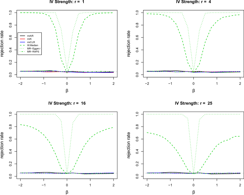
Figure 1: Size under different IV strength. The number of instruments is $L=100$. $r$ represents instrument strength, with higher indicating stronger instruments; $r$ approximately corresponds to the first-stage F statistic for IV strength. The grey dashed horizontal line represents the Type I error rate of $0.05$. This figure appears in color in the electronic version of this article, and any mention of color refers to that version.

Next, Figure 2 examines statistical power when the null hypothesis is $H_{0}:\beta=0$ (left panel) or $H_{0}:\beta=1$ (right panel); the significance level is set at $\alpha=0.05$. Under the null hypothesis of no effect $H_{0}:\beta=0$, all methods correctly control the Type I error for every value of $r$ and every method except MR-Egger.r has similar statistical power when $r=16$ or $r=25$. However, for lower values of $r$, mrK and mrCLR have superior statistical power, with mrCLR having the best power among all methods; this agrees with Andrews et al., (2006) who showed that the CLR test in the single-sample individual-data setting is nearly optimal. Under $H_{0}:\beta=1$, none of the pre-existing methods except MR-RAPS have Type I error control for every value of $r$. In contrast, our tests always maintain Type I error control and mrCLR has the best power among all existing methods presented in the simulation study. Section 1.1 of the supplementary materials repeats the simulation above with $r=50$ and the results are similar to the case when $r=25$.

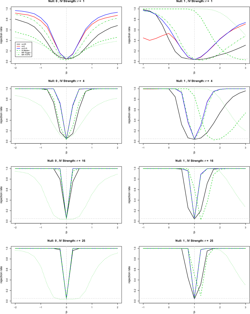
Figure 2: Power curves under different nulls and IV strength. The left panel is under $H_{0}:\beta=0$ and the right panel is under $H_{0}:\beta=1$; each null value is represented by a grey dashed vertical line. $r$ represents instrument strength, with higher indicating stronger instruments; $r$ approximately corresponds to the first-stage F statistic for IV strength. The grey dashed horizontal line represents the Type I error rate of $0.05$. This figure appears in color in the electronic version of this article, and any mention of color refers to that version.

Overall, our tests always retain size control for different values of $r$ and null values $\beta_{0}$. Additionally, mrCLR has the best power among existing methods when $r$ is low and has no worse power than existing methods when $r$ is high. In short, mrCLR does well under both weak and strong instruments.

3.2 mrAR Under Invalid Instruments

In this section, we explore mrAR’s ability to detect a wide variety of invalid instruments under different $r$. The simulation model is generated from the structural model:

$$\begin{split}&\ Y_{li}=\beta_{\rm int}+D_{li}\beta+Z_{li}^{\intercal}\alpha+\epsilon_{li},\quad{}D_{li}=\gamma_{\rm int}+Z_{li}^{\intercal}\gamma+\delta_{li},\quad{}E[\epsilon_{li},\delta_{li}\mid Z_{li}]=0.\end{split}$$ (3)

Compared to model (1), model (3) includes $\alpha$, which is the direct effect of the instruments $Z_{li}$ on the outcome $Y_{li}$. If $\alpha=0$, there is no direct effect and all instruments are valid. If $\alpha\neq 0$, instruments with $\alpha_{j}\neq 0$ have direct effects on the outcome and are invalid; see Kang et al., (2016) and Bowden et al., 2016b for additional discussions of defining invalid IVs.

For the simulation study, we vary the number of invalid instruments, i.e. $\sum_{j=1}^{L}I(\alpha_{j}\neq 0)$, from 10% of $L$ to 90% of $L$. We also vary the magnitude of $\alpha_{j}$ to be either $0.003$, $0.01$, or $0.05$; $0.003$ roughly corresponds to $\alpha_{j}\approx 1/\sqrt{n_{1}}$, or essentially local-to-zero invalid instruments, $0.05$ roughly corresponds to $\alpha_{j}\approx 1/n_{1}^{1/4}$, or non-local invalid instruments, and $0.01$ is somewhere in between these types of invalid instrument. The invalid instruments do not satisfy the Instrument Strength Independent of Direct Effect (InSIDE) assumption (Bowden et al.,, 2015). Also, when less than 50% of the instruments are invalid, the majority and the plurality assumptions (Guo et al.,, 2018) are satisfied. When 50% or more of the instruments are invalid, they are not satisfied. The true causal effect $\beta$ is set at $0.5$. and we test $H_{0}:\beta=\beta_{0}$ against $H_{1}:\beta\neq\beta_{0}$ where $\beta_{0}$ ranges from $-4$ to $5$. The other parameters of the simulation settings remain the same as before. Finally, for comparison, we use the modified second-order weighting Q statistic in Bowden et al., (2019), which was designed to test for invalid instruments.

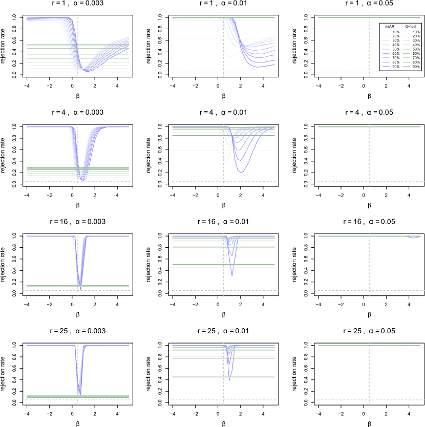
Figure 3: Rejection rates of mrAR and Q-test under invalid instruments. The true value of $\beta$ is represented by the vertical grey line at $0.5$ and we test $H_{0}:\beta=\beta_{0}$ for different values of $\beta_{0}$. $r$ represents instrument strength, with higher indicating stronger instruments; $r$ approximately corresponds to the first-stage F statistic for IV strength. Each column changes the magnitude of $\alpha$ from $0.003$ to $0.05$. Each purple or green line represents the proportion of invalid IVs as measured by the number of $\alpha_{j}\neq 0$ divided by $L$. The grey horizontal line represents the Type I error rate of $0.05$. This figure appears in color in the electronic version of this article, and any mention of color refers to that version.

Figure 3 shows the rejection rates of mrAR and the Q statistic at each value of $\beta_{0}$ under different configurations of $\alpha$. Note that because the Q statistic tests the null hypothesis of heterogeneous effect and doesn’t rely on a null value $\beta_{0}$ for the true effect, it shows a flat rejection rate across $\beta_{0}$. For different types of $\alpha$ and instrument strength $r$, mrAR remains above the $0.05$ threshold across all $\beta_{0}$, thereby always rejecting the null hypothesis and returning empty confidence intervals to alert investigators about potentially invalid instruments. The mrAR test rejects more frequently when $\alpha$ is farther away from zero or when instrument strength increases. For example, if $\alpha_{j}=0.05$, which is roughly on the order of $1/n_{1}^{1/4}$, mrAR always rejects at 100% regardless of the proportion of invalid instruments. The result of the Q statistic is similar to the mrAR as the Q statistic remains above the $0.05$ threshold for all values of $r$. Also, similar to mrAR, the Q statistic has a higher rejection rate when the magnitude of $\alpha_{j}$ grows. Web Appendix A of the supporting information repeats the simulation above with $r=50$ and another test statistic by Bowden et al., (2019) and the results are similar to the case when $r=25$. Overall, we believe both mrAR and the Q statistic are useful in detecting invalid instruments under a wide variety of settings and could be used as pre-tests for methods that are sensitive to invalid instruments.

3.3 Correlated Instruments

In this section, we assess our proposed tests under correlated instruments, especially demonstrating our adjustment procedure in Section 2.3 and the procedure’s performance under incorrectly specified correlation matrices $M_{l}$. Under model (1) and for each $l=1,2$, we set the diagonal elements of $M_{l}$ as $1$ and the non-diagonal, $ij$th element of $M_{l}$ as $\rho=0.3$ if $\lvert i-j\rvert=1$, and $0$ if $\lvert i-j\rvert\geq 2$; in short, adjacent SNPs are correlated with correlation coefficient $\rho=0.3$. For each $l$, we let $\widehat{M}_{l}$ denote our working value of $M_{l}$ and use it in our adjustment procedure. If $\widehat{M}_{l}=M_{l}$, we say that the correlation matrix $\widehat{M}_{l}$ is correctly specified and if $\widehat{M}_{l}\neq M_{l}$, the correlation matrix is incorrectly specified.

For incorrect specifications of $\widehat{M}_{l}$, we assume the zero elements of $\widehat{M}_{l}$ are the same as $M_{l}$, but the non-zero, off-diagonal elements differ, taking on values $\hat{\rho}\in\{0,0.2,0.3,0.4\}$. When $\hat{\rho}<\rho=0.3$, the investigator is assuming there is little to no correlation between instruments, even though in reality, instruments are actually correlated. When $\hat{\rho}>\rho=0.3$, the investigator is assuming there is a stronger correlation than the true correlation of $0.3$. When $\hat{\rho}=\rho=0.3$, the investigator has correctly specified the true correlation. The other parameters are the same as in Section 3.1 except we only look at $r=1$ to assess our proposed tests in the hardest scenario for instrument strength; Section 1.3 of the supplementary materials contain cases when $r$ is higher and shows similar results.

Figure 4 shows the size and power of our tests based on the adjustment procedure described in Section 2.3. We see that if $\hat{\rho}\leq\rho$, our adjusted tests have a slight size inflation not exceeding 10% across different values of $\beta_{0}$. Also, the size inflation decreases as $\hat{\rho}$ gets close to $\rho$. For power, mrCLR has the best power among the three tests. When $\hat{\rho}=\rho$, our adjusted tests have size control at level $\alpha$, as predicted by Theorem 2, and exhibit the same behavior demonstrated in Section 3.1. However, when $\hat{\rho}>\rho$, the size distortion of our adjusted tests ranges from $1\%$ to $25\%$, with mrK and mrCLR having the smallest size distortions.

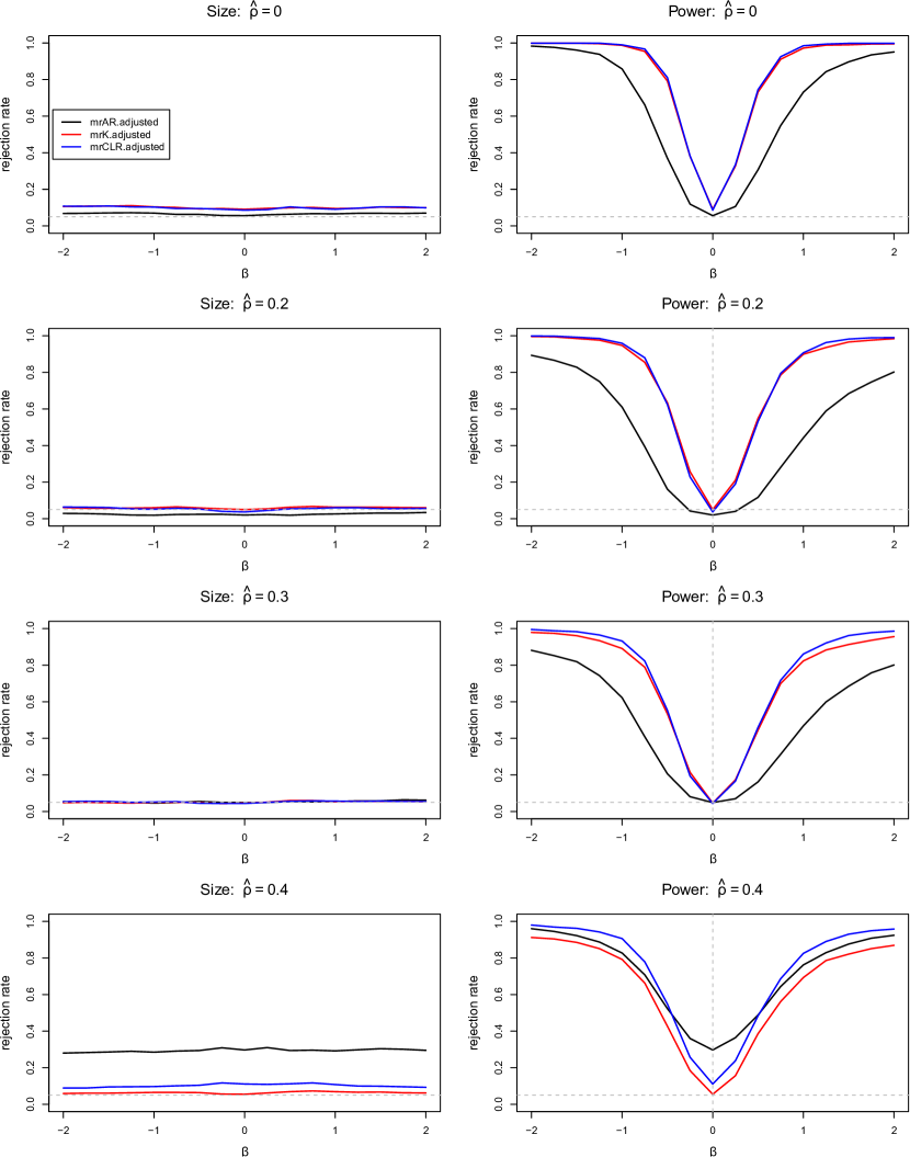
Figure 4: Performance of proposed tests with correlated instruments when $r=1$. The left panel shows size and the right panel shows power of testing $H_{0}:\beta=0$. The true correlation $\rho$ is $0.3$ and each row changes the magnitude of $\hat{\rho}$ from $0$ to $0.4$. The true value of $\beta$ in the power plot is represented by a grey dashed vertical line at $0$. The grey dashed horizontal line represents the Type I error rate of $0.05$. This figure appears in color in the electronic version of this article, and any mention of color refers to that version.

Web Appendix A of the supporting information explores other mis-specifications of the correlation matrix, notably the case where we mis-specify the zero elements. Overall, while the simulation studies do not capture every possible mis-specification, the main takeaway message is that if an investigator has access to reasonable estimates of the correlation matrices, he/she should use the proposed adjustment procedure for our tests. However, if there is uncertainty about the correlation matrices, he/she should proceed as if there is no correlation between the instruments, even though in reality they are actually correlated. In this case, the sizes of our $0.05$ level tests are modestly inflated, with sizes ranging from 1% to 10%. In contrast, if one adjusts our tests for correlation even though there isn’t any correlation between instruments, the size distortions range from 1% to 25%.

4 Data Analysis

4.1 Replication of Zhao et al., (2020)’s Empirical Study

To validate our methods in real data, we replicate an analysis by Zhao et al., (2020) on the effect of BMI on systolic blood pressure where the effect was known to be positive. The authors used three independent GWAS, one from the UK Biobank GWAS (SBP-UKBB) and the other two from GWAS by the Genetic Investigation of ANthropometric Traits (GIANT) consortium (Locke et al.,, 2015). Specifically, the “BMI-MAL” and “SBP-UKBB” datasets in Zhao et al., (2020) provided summary statistics of the IV-exposure and IV-outcome statistics, respectively. The “BMI-FEM” dataset from Zhao et al., (2020) was used to pre-screen for strong and uncorrelated IVs. This pre-screening dataset led to two sets of instruments, a set of 160 instruments based on the p-value threshold of $10^{-4}$ and another set of 25 instruments based on the genome-wide significance level of $5\cdot 10^{-8}$; the latter is also the default setting for selecting instruments in the MR-Base platform (Hemani et al.,, 2018). In both sets of instruments, each pair of instruments were at least 10,000 kilobases apart and had linkage disequilibrium correlation coefficients less than $0.001$; see Zhao et al., (2020) for more details..

We compute 95% confidence intervals using mrAR, mrK, mrCLR, W.Median, MR-Egger.r, and two versions of MR-RAPS, MR-RAPS with a square error loss (MR-RAPS) and MR-RAPS with a huber loss (MR-RAPS.r). We also computed the F statistic typical in IV studies to measure instrument strength. Specifically, in Web Appendix A of the supporting materials, we show that if the instruments are independent of each other, the usual F statistic in linear IV models can be computed from two-sample summary-data MR by using the formula

$$F=\left(\frac{n_{2}-L+1}{L}\right)\left(\frac{\sum_{i=1}^{L}\frac{F_{i}}{F_{i}+n_{2}-L-1}}{1-\sum_{i=1}^{L}\frac{F_{i}}{F_{i}+n_{2}-L-1}}\right)$$

where $F_{i}=\widehat{\gamma}_{i}^{2}/\Sigma_{\gamma,ii}$ is the square of the t-statistic for instrument $i$, or equivalently the F statistic for instrument $i$. If $n_{2}-L$ is sufficiently large enough, we can approximate the $F$ statistic as the average of $F_{i}$s, i.e. $F\approx L^{-1}\sum_{i=1}^{L}F_{i}$; this latter approximation has been mentioned in prior works (Bowden et al.,, 2019) and our exposition in the supplementary materials provide a formal justification to this approximation.

Table 1: 95% confidence intervals of the effect of body mass index on systolic blood pressure from Zhao et al., (2020). The thresholds refer to significance thresholds used in Zhao et al., (2020)’s analysis to select instruments.

	25 Instruments ($5\times 10^{-8}$ Threshold)	160 Instruments ($10^{-4}$ Threshold)
${\rm mrK}$	(0.205, 0.530)	(0.377, 0.771)
${\rm mrCLR}$	(0.211, 0.524)	(0.415, 0.731)
${\rm mrAR}$	($\emptyset$)	($\emptyset$)
W.Median	(0.278, 0.762)	(0.318, 0.726)
MR-Egger.r	(0.075, 1.038)	(0.203, 0.573)
MR-RAPS	(0.221, 0.514)	(0.499, 0.712)
MR-RAPS.r	(0.097, 0.610)	(0.141, 0.615)
F statistic	58.140	25.462
Q statistic (p-value)	5.582 $\times 10^{-8}$	5.727$\times 10^{-61}$

Table 1 summarizes our results and two interesting observations emerge from the re-analysis of Zhao et al., (2020)’s dataset. First, almost all methods have overlapping 95% confidence intervals, despite both mrAR and the Q statistic alerting investigators that invalid instruments may be present. Specifically, mrK and mrCLR, which are not robust to invalid instruments, generate similar confidence intervals as methods that are robust to invalid instruments, notably W.Median, MR-Egger.r, and MR-RAPS.r. This suggests either that invalid instruments are present, but small or, as Small and Rosenbaum, (2008) suggests, when IVs are weak, the first-order bias is dominated by weak IVs and therefore, correcting for weak-IV bias through weak-IV robust methods like ours can attenuate biases from invalid IVs. Note that Table 1 only reports the positive region since we know a priori that the effect is positive; in general, when the exposure effect direction is unknown, we recommend taking the union of the disjoint intervals.

4.2 Validation: Testing the Null of No Effect

Given that the effect of BMI on SBP is generally thought to be positive, we validate our analysis above by testing the null hypothesis of no exposure effect (i.e $H_{0}:\beta=0$), but with an increasing set of strong instruments. Testing the null of no effect is one of the first questions that an MR investigator may ask about the study and for the BMI study, an ideal test should reject the null regardless of the strength of the instruments. In other words, when we go from the weakest set of instruments to all 160 instruments, an ideal test should reject the null of no effect by generating a p-value that is less than $\alpha=0.05$. We remark that this validation analysis is similar in spirit to the power simulations in Section 3.1 where we are examining the power to reject the null of no effect in favor of a known true alternative.

Figure 5 plots the p-values from testing this null hypothesis as a function of the F statistic and the number of instruments, arranged in increasing order of strength. We see that mrCLR always rejects the null hypothesis of no effect of BMI on blood pressure at $\alpha=0.05$ level, even with the 3 weakest IVs (left end of the x-axis), while other MR methods cannot reject the null hypothesis unless more strong IVs are present. mrAR and mrK also have smaller p-values for testing the null than existing methods across all instrument strength. These observations also confirm our simulation study in Section 3.1 where mrCLR exhibited superior power compared to existing methods. However, as a practical matter, we caution that relying solely on p-values to establish a causal effect can potentially be misleading since they don’t tell the magnitude of the true effect nor reveal the direction of potential biases.

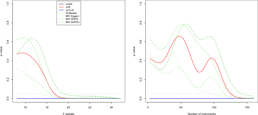
Figure 5: P-values for testing the null hypothesis of no exposure effect under different number of instruments and strength. We plot a smoothed curve of p-values using a Gaussian kernel with the p-values’ standard deviation as the smoothing parameter; this is the default value in the sm.regression()+ function in the R package sm+. The grey dashed horizontal line represents the rejection threshold at $0.05$. The number of instruments goes from $3$ weakest instruments to all $160$ instruments. This figure appears in color in the electronic version of this article, and any mention of color refers to that version.

4.3 Validation: Stress Testing Based on Bound et al., (1995)

To further validate our analysis, we follow an approach by Bound et al., (1995) where we “stress-test” methods by replacing each of the original IV-exposure effects $\widehat{\gamma}_{j}$ and the IV-outcome effects $\widehat{\Gamma}_{j}$ for the set of 160 instruments by $\widehat{\gamma}_{j}^{\rm new}\sim N(K\widehat{\gamma}_{j},\widehat{\Sigma}_{\gamma,j})$ and $\widehat{\Gamma}_{j}^{\rm new}\sim N(K\widehat{\gamma}_{j}\beta,\widehat{\Sigma}_{\Gamma,j})$; here, $\beta$, the true exposure effect, is set to be $0.5$ and $1.5$. The parameter $K$ controls IV strength and ranges from $0$ to $1$. Under $K=1$, the new IV-exposure and IV-outcome effects are essentially the original effects, but with a known true value of $\beta$. But, as $K$ decreases to $0$, the IV becomes weaker than the original ones. In the extreme case when $K=0$, there is no way to consistently estimate $\beta$; the new IV-exposure and IV-outcome effects look statistically indistinguishable if the true exposure effect is $\beta=1$ or $\beta=1000$.

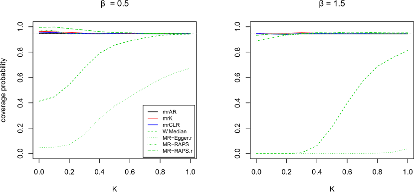
Figure 6: Coverage probability under different IV strength. The left panel sets the true causal effect $\beta$ to be 0.5 and the right panel sets $\beta$ to be 1.5. The grey dashed horizontal line represents $95\%$ coverage. This figure appears in color in the electronic version of this article, and any mention of color refers to that version.

An ideal confidence interval should be able to (i) automatically detect the lack of identification of the exposure effect $\beta$ by producing an infinite confidence interval when $K=0$ 95% of the time to maintain a 95% coverage rate and (ii) a bounded confidence interval with a 95% coverage rate when $K$ moves away from zero; in short, it should produce 95% coverage rates across all values of $K$. As Figure 6 shows, the existing MR methods do not achieve these two goals. For example, when $K=0$ and $\beta=0.5$, W.Median, MR-Egger.r, MR-RAPS, and MR-RAPS.r produced bounded intervals across 1,000 simulations even though $\beta$ is not identifiable. We remark that it is by luck that MR-RAPS’ confidence intervals produced large, bounded intervals to cover the true effect of $\beta$ of $0.5$ even though $\beta$ is not identifiable in this scenario. Indeed, in the right-hand plot of Figure 6 when $K=0$ and $\beta=1.5$, W.Median, MR-Egger.r, MR-RAPS, and MR-RAPS.r again produced bounded intervals, but their coverage rates drop, sometimes dramatically, because the true effect is farther away from $0$. In contrast, mrAR, mrK, and mrCLR produced infinite confidence intervals when $K=0$ around 95% of the time to maintain 95% coverage. More generally, our tests always maintained a 95% coverage rate across all values of $K$ and $\beta$ and satisfied the two criteria (i) and (ii).

5 Summary, Limitations, and Recommendations

In this paper, we propose weak-IV robust test statistics for two-sample summary data in MR by extending the existing AR, Kleibergen, and CLR tests in econometrics and show that they have Type I error control under weak instrument asymptotics. The simulation results show that if there is no evidence of pleiotropy, then among existing tests designed for weak instruments, mrCLR is superior. Similarly, the replication of the data analysis in Zhao et al., (2020) and the two validation analyses echoed findings from the simulation studies.

While this work is focused on weak instruments in MR and using powerful tests from econometrics to address them, a major concern in MR is the presence of invalid instruments. Invalid instruments would violate Assumption (A2) and can bias our confidence intervals. However, as we saw in the replication analysis in Section 4.1, the intervals from our methods, which are not robust to invalid instruments, were similar to those from methods that are robust to invalid instruments, suggesting that invalid instruments had little impact in this particular study or, as mentioned earlier, correcting for weak-IV bias through weak-IV robust methods like ours can attenuate biases from invalid IVs.

Web Appendix A of the supporting information conducts a simulation study to assess the sensitivity of our methods under various types of invalid instruments. In summary, the results show that mrK and mrCLR are reasonably robust against invalid instruments when the direct effects are small. But, they are significantly biased as the magnitude of the direct effects and the number of invalid instruments increase; we also show that other robust methods, notably MR-RAPS.r, suffer in this setting as well. Thankfully, as Section 3.2 showed, mrAR is able to detect invalid instruments in a variety of settings and can be used as a pre-screening test before using our methods; see Kang et al., (2020) for details.

We conclude by making some recommendations about how to use our methods in practice. First, from the simulation results and the data analysis above, we recommend practitioners start by using mrAR or the Q statistic to check for invalid instruments, especially if the instruments are weak. Second, if mrAR returns non-empty confidence intervals and thus, the instruments are plausibly valid, we recommend investigators use mrCLR. Additionally, mrCLR is the only test that we know in the two-sample summary-data MR which satisfies Dufour, (1997)’ necessary condition for valid confidence intervals and adapts to produce infinite confidence intervals, if necessary. Third, if mrAR returns empty confidence intervals, suggesting a presence of invalid instruments, there is currently no method that can be robust to every parametrization of invalid instruments. As such, we recommend practitioners follow what we did in our empirical analysis and use a combination of methods. In particular, as we saw in the empirical example above, even though mrAR returned an empty confidence interval and suggested invalid instruments were present, the confidence intervals generated from mrCLR and mrK were similar to those from methods that are robust to invalid instruments, say MR-RAPS with a robust loss function, and comparing the confidence intervals between these methods yielded some understanding about the type of invalid instruments present in the study. Fourth, from our investigation into correlated instruments, when using our tests, if the pairwise correlation between instruments is unknown, we generally recommend investigators proceed as if instruments aren’t correlated, even if in reality they are actually correlated, as this strategy tends to lead to only modest size distortions.

Data Availability Statement

The data that support the findings of this paper are openly available in CRAN at https://cran.r-project.org/package=mr.raps, reference number (Zhao,, 2018).

References

- Anderson et al., (1949) Anderson, T. W., Rubin, H., et al. (1949). Estimation of the parameters of a single equation in a complete system of stochastic equations. The Annals of Mathematical Statistics, 20(1):46–63.
- Andrews et al., (2006) Andrews, D. W., Moreira, M. J., and Stock, J. H. (2006). Optimal two-sided invariant similar tests for instrumental variables regression. Econometrica, 74(3):715–752.
- Bound et al., (1995) Bound, J., Jaeger, D. A., and Baker, R. M. (1995). Problems with instrumental variables estimation when the correlation between the instruments and the endogenous explanatory variable is weak. Journal of the American Statistical Association, 90(430):443–450.
- Bowden et al., (2015) Bowden, J., Davey Smith, G., and Burgess, S. (2015). Mendelian randomization with invalid instruments: effect estimation and bias detection through Egger regression. International Journal of Epidemiology, 44(2):512–525.
- (5) Bowden, J., Davey Smith, G., Haycock, P. C., and Burgess, S. (2016a). Consistent estimation in Mendelian randomization with some invalid instruments using a weighted median estimator. Genetic Epidemiology, 40(4):304–314.
- Bowden et al., (2017) Bowden, J., Del Greco M, F., Minelli, C., Davey Smith, G., Sheehan, N., and Thompson, J. (2017). A framework for the investigation of pleiotropy in two-sample summary data Mendelian randomization. Statistics in Medicine, 36(11):1783–1802.
- (7) Bowden, J., Del Greco M, F., Minelli, C., Davey Smith, G., Sheehan, N. A., and Thompson, J. R. (2016b). Assessing the suitability of summary data for two-sample Mendelian randomization analyses using MR-Egger regression: the role of the I 2 statistic. International Journal of Epidemiology, 45(6):1961–1974.
- Bowden et al., (2019) Bowden, J., Del Greco M, F., Minelli, C., Zhao, Q., Lawlor, D. A., Sheehan, N. A., Thompson, J., and Davey Smith, G. (2019). Improving the accuracy of two-sample summary-data Mendelian randomization: moving beyond the NOME assumption. International Journal of Epidemiology, 48(3):728–742.
- Bowden et al., (2018) Bowden, J., Spiller, W., Del Greco M, F., Sheehan, N., Thompson, J., Minelli, C., and Davey Smith, G. (2018). Improving the visualization, interpretation and analysis of two-sample summary data Mendelian randomization via the Radial plot and Radial regression. International Journal of Epidemiology, 47(4):1264–1278.
- Burgess et al., (2013) Burgess, S., Butterworth, A., and Thompson, S. G. (2013). Mendelian randomization analysis with multiple genetic variants using summarized data. Genetic Epidemiology, 37(7):658–665.
- Burgess et al., (2016) Burgess, S., Dudbridge, F., and Thompson, S. G. (2016). Combining information on multiple instrumental variables in Mendelian randomization: comparison of allele score and summarized data methods. Statistics in Medicine, 35(11):1880–1906.
- Burgess et al., (2015) Burgess, S., Scott, R. A., Timpson, N. J., Smith, G. D., Thompson, S. G., Consortium, E.-I., et al. (2015). Using published data in Mendelian randomization: a blueprint for efficient identification of causal risk factors. European Journal of Epidemiology, 30(7):543–552.
- Burgess and Thompson, (2011) Burgess, S. and Thompson, S. G. (2011). Bias in causal estimates from Mendelian randomization studies with weak instruments. Statistics in Medicine, 30(11):1312–1323.
- Choi et al., (2018) Choi, J., Gu, J., and Shen, S. (2018). Weak-instrument robust inference for two-sample instrumental variables regression. Journal of Applied Econometrics, 33(1):109–125.
- Davey Smith and Ebrahim, (2003) Davey Smith, G. and Ebrahim, S. (2003). “Mendelian randomization”: can genetic epidemiology contribute to understanding environmental determinants of disease? International Journal of Epidemiology, 32(1):1–22.
- Davidson and MacKinnon, (2014) Davidson, R. and MacKinnon, J. G. (2014). Confidence sets based on inverting Anderson–Rubin tests. The Econometrics Journal, 17(2):S39–S58.
- Dufour, (1997) Dufour, J.-M. (1997). Some impossibility theorems in econometrics with applications to structural and dynamic models. Econometrica: Journal of the Econometric Society, pages 1365–1387.
- Guo et al., (2018) Guo, Z., Kang, H., Tony Cai, T., and Small, D. S. (2018). Confidence intervals for causal effects with invalid instruments by using two-stage hard thresholding with voting. Journal of the Royal Statistical Society: Series B (Statistical Methodology), 80(4):793–815.
- Hartwig et al., (2017) Hartwig, F. P., Davey Smith, G., and Bowden, J. (2017). Robust inference in summary data Mendelian randomization via the zero modal pleiotropy assumption. International Journal of Epidemiology, 46(6):1985–1998.
- Hemani et al., (2018) Hemani, G., Zheng, J., Elsworth, B., Wade, K. H., Haberland, V., Baird, D., Laurin, C., Burgess, S., Bowden, J., Langdon, R., et al. (2018). The MR-Base platform supports systematic causal inference across the human phenome. Elife, 7:e34408.
- Holland, (1988) Holland, P. W. (1988). Causal inference, path analysis and recursive structural equations models. ETS Research Report Series, 1988(1):i–50.
- Johnson et al., (2008) Johnson, A. D., Handsaker, R. E., Pulit, S. L., Nizzari, M. M., O’Donnell, C. J., and De Bakker, P. I. (2008). SNAP: a web-based tool for identification and annotation of proxy SNPs using HapMap. Bioinformatics, 24(24):2938–2939.
- Kang et al., (2020) Kang, H., Lee, Y., Cai, T. T., and Small, D. S. (2020). Two robust tools for inference about causal effects with invalid instruments. Biometrics.
- Kang et al., (2016) Kang, H., Zhang, A., Cai, T. T., and Small, D. S. (2016). Instrumental variables estimation with some invalid instruments and its application to Mendelian randomization. Journal of the American Statistical Association, 111(513):132–144.
- Kleibergen, (2002) Kleibergen, F. (2002). Pivotal statistics for testing structural parameters in instrumental variables regression. Econometrica, 70(5):1781–1803.
- Lawlor et al., (2008) Lawlor, D. A., Harbord, R. M., Sterne, J. A., Timpson, N., and Davey Smith, G. (2008). Mendelian randomization: using genes as instruments for making causal inferences in epidemiology. Statistics in Medicine, 27(8):1133–1163.
- Locke et al., (2015) Locke, A. E., Kahali, B., Berndt, S. I., Justice, A. E., Pers, T. H., Day, F. R., Powell, C., Vedantam, S., Buchkovich, M. L., Yang, J., et al. (2015). Genetic studies of body mass index yield new insights for obesity biology. Nature, 518(7538):197.
- Moreira and Moreira, (2019) Moreira, H. and Moreira, M. J. (2019). Optimal two-sided tests for instrumental variables regression with heteroskedastic and autocorrelated errors. Journal of Econometrics, 213(2):398–433.
- Moreira, (2003) Moreira, M. J. (2003). A conditional likelihood ratio test for structural models. Econometrica, 71(4):1027–1048.
- Pierce and Burgess, (2013) Pierce, B. L. and Burgess, S. (2013). Efficient design for Mendelian randomization studies: subsample and 2-sample instrumental variable estimators. American Journal of Epidemiology, 178(7):1177–1184.
- Small and Rosenbaum, (2008) Small, D. S. and Rosenbaum, P. R. (2008). War and wages: the strength of instrumental variables and their sensitivity to unobserved biases. Journal of the American Statistical Association, 103(483):924–933.
- Staiger and Stock, (1997) Staiger, D. and Stock, J. H. (1997). Instrumental variables regression with weak instruments. Econometrica, 65:557–586.
- Stock et al., (2002) Stock, J. H., Wright, J. H., and Yogo, M. (2002). A survey of weak instruments and weak identification in generalized method of moments. Journal of Business & Economic Statistics, 20(4):518–529.
- Windmeijer, (2019) Windmeijer, F. (2019). Two-stage least squares as minimum distance. The Econometrics Journal, 22(1):1–9.
- Yavorska and Burgess, (2017) Yavorska, O. O. and Burgess, S. (2017). MendelianRandomization: an R package for performing Mendelian randomization analyses using summarized data. International Journal of Epidemiology, 46(6):1734–1739.
- Ye et al., (2019) Ye, T., Shao, J., and Kang, H. (2019). Debiased inverse-variance weighted estimator in two-sample summary-data mendelian randomization. arXiv preprint arXiv:1911.09802.
- Zhao, (2018) Zhao, Q. (2018). mr.raps: Two sample mendelian randomization using robust adjusted profile score. CRAN, (Version 0.2).
- Zhao et al., (2019) Zhao, Q., Wang, J., Bowden, J., and Small, D. S. (2019). Two-sample instrumental variable analyses using heterogeneous samples. Statistical Science, 34(2):317–333.
- Zhao et al., (2020) Zhao, Q., Wang, J., Hemani, G., Bowden, J., Small, D. S., et al. (2020). Statistical inference in two-sample summary-data Mendelian randomization using robust adjusted profile score. Annals of Statistics, 48(3):1742–1769.