Pointer-based Fusion of Bilingual Lexicons into Neural Machine Translation

Abstract

Neural machine translation (NMT) systems require large amounts of high quality in-domain parallel corpora for training. State-of-the-art NMT systems still face challenges related to out of vocabulary words and dealing with low-resource language pairs. In this paper, we propose and compare several models for fusion of bilingual lexicons with an end-to-end trained sequence-to-sequence model for machine translation. The result is a fusion model with two information sources for the decoder: a neural conditional language model and a bilingual lexicon. This fusion model learns how to combine both sources of information in order to produce higher quality translation output. Our experiments show that our proposed models work well in relatively low-resource scenarios, and also effectively reduce the parameter size and training cost for NMT without sacrificing performance.

1 Introduction

Recent years have seen rapid progress in neural machine translation (NMT) research. While fully neural systems with attention mechanism (Bahdanau et al., 2014; Luong et al., 2015a; Vaswani et al., 2017) achieve the state-of-the-art performance on several benchmarks, digesting large source and target side vocabulary sets remains a major challenge. Neural models rely on either word embedding matrices or character-level encoders, which constrains the ability of the models of handling unseen or rare words. For word-embedding-based NMT, models commonly treat these words (including named entities) as Out-of-Vocabulary (OOV) and replace with a unified UNK token. Meanwhile, language naturally evolves through time. Adaptation to such evolution for a neural model can mean laborious gathering of new data and fine-tuning millions of parameters. Sensitive domains such as Biomedical also require high precision terminology translation that is hard to guarantee in neural space.

An intuitive way to tackle these issue is to utilise a copy mechanism or separate transliteration mechanism. Luong et al. (2015b) propose UNK replacement based on Pointer Network (Vinyals et al., 2015). After neural decoding, the model replaces UNK tokens by looking up the source word with highest attention score and copying it over. Gulcehre et al. (2016) propose to use pointer generator to determine when to copy, and a separate pointer scoring layer instead of attention scores. Li et al. (2018); Wang et al. (2017) focus on named entities by adding a separate char-level transliteration model. This line of work however, does not cover more general lexical categories.

In this paper, we propose a novel way to combine prior knowledge from a dictionary-like bilingual lexicon with a fully neural translation model. We extend pointer-based copy with a translation table (dictionary) and its entry-level features. Such knowledge are all automatically generated from the training data, although we also demonstrate that the inclusion of external knowledge is also possible and beneficial. The result is a fusion model with a contextual neural language model combined with a bilingual lexicon. Our experimental results show that our fusion model retains translation quality when the number of its neural parameters is dramatically reduced to even a fourth of the original size.

2 Related Work

The subject of utilising external lexical knowledge has been an interesting topic for NMT.

Jean et al. (2015); Mi et al. (2016) use a dictionary to limit the target search space, improving inference efficiency. Hokamp and Liu (2017); Post and Vilar (2018) enforce lexical constraints in beam search. Hasler et al. (2018) further uses finite-state acceptors in beam search to ensure decoding conforms to multiple lexical constraints. The decoder here is influenced by an external scoring function that is knowledge-aware, improving interpretability and flexibility. Although as Chatterjee et al. (2017) claim, the fact that the neural model is unaware of the lexical constraints may lead to sub-optimal translation.

Alternatively, Arthur et al. (2016) investigate using the alignment scores as regularisers. The distilled lexical knowledge is incorporated into the probability distribution calculation as a bias term.

A separate line of work focuses on data manipulation. Arcan et al. (2015) use the bilingual anthology to filter out domain-irrelevant samples for training. Song et al. (2019) also perform data synthesis by replacing the source rare words with their translations from a bilingual lexicon.

3 Neural Machine Translation and Copy Mechanism

Machine translation are models for which the input token sequence $X=(x_{0},x_{1},...,x_{n-1})$ in language 1 (source) is transformed into its semantically equivalent output sequence $Y=(y_{0},y_{1},...,y_{m-1})$ in a second language (target). Neural machine translation models are ones in which the conditional language model $\operatorname{P}(Y|X)$ is computed using neural networks.

Common NMT models use encoder-decoder architecture (Sutskever et al., 2014). The encoder transforms the input into hidden representation space, to be taken by the decoder as input to generate the final output (distribution). The baseline model we use in this paper is a sequence-to-sequence model under such architecture with attention (Bahdanau et al., 2014; Luong et al., 2015a). The encoder and decoder are both LSTM units (Hochreiter and Schmidhuber, 1997), more specifically the encoder is a bidirectional LSTM that processes the input sequence from both directions (Equation 1).

$$\overrightarrow{h}^{\operatorname{enc}}_{i} =\overrightarrow{\operatorname{LSTM}}(\overrightarrow{h}^{\operatorname{enc}}_{i-1},x_{i})$$ (1)

$$\overleftarrow{h}^{\operatorname{enc}}_{i} =\overleftarrow{\operatorname{LSTM}}(\overleftarrow{h}^{\operatorname{enc}}_{i+1},x_{i})$$

$$h^{\operatorname{enc}}_{i} =[\overrightarrow{h}^{\operatorname{enc}}_{i};\overleftarrow{h}^{\operatorname{enc}}_{i}]$$

Then, at each step $t$, attention mechanism takes as input the decoder state $h^{\operatorname{dec}}_{t}$ and all encoder states to generate context vector $c_{t}$ (Equation 2).

$$\mathrm{score}_{ti} =V\times\tanh(W\times h^{\operatorname{dec}}_{t}+U\times h^{\operatorname{enc}}_{i})$$ (2)

$$\alpha_{t} =\operatorname{softmax}(\mathrm{score}_{t})$$

$$c_{t} =\sum_{i}\alpha_{ti}h^{\operatorname{enc}}_{i}$$

Finally, $c_{t}$ and $h^{\operatorname{dec}}_{t}$ are combined to calculate the probability distribution over the neural lexicon (Equation 3). After that, decoding continues by feeding both representations and the generated word’s embedding back into the decoder, until a end-of-sequence token is omitted.

$$h^{\operatorname{dec}}_{t} =\operatorname{LSTM}^{\operatorname{dec}}(\hat{h}^{\operatorname{dec}}_{t-1},y_{t-1})$$ (3)

$$\hat{h}^{\operatorname{dec}}_{t} =\tanh(C\times[c_{t};h^{\operatorname{dec}}_{t}])$$

$$\operatorname{P}_{\operatorname{dec}}(y_{t}=w|y_{<t},X) =\operatorname{softmax}(\operatorname{affine}(\hat{h}^{\operatorname{dec}}_{t}))(w)$$

Gulcehre et al. (2016); Gu et al. (2016); See et al. (2017) proposes pointer generator (PG), which is essentially a switch that determines at each step $t$, whether to use the neural decoder’s output or to copy. We formulate PG using an activation unit $p_{gen}$ (Equation 4, the probability of using neural generation).

$$p_{gen} =\sigma(w_{gen}^{T}c_{t}+b_{gen})$$ (4)

$$\operatorname{P}_{\mathrm{CopyPG}}(y_{t}=w |y_{<t},X)=$$

$$p_{gen} \times\operatorname{P}_{\operatorname{dec}}(y_{t}=w|y_{<t},X)+$$

$$(1-p_{gen}) \times\sum_{x_{i}=w}\alpha_{i}$$

During inference, when $p_{gen}$ is bigger than a certain threshold (we find using extensive experimentation that 0.5 works the best) the model uses the neural decoder’s output, otherwise the copy mechanism is triggered. The word copied from source is $\operatorname{argmax}_{i}\alpha_{i}$ entry $x_{i}$.

4 Dictionary Fusion

(Luong et al., 2015b; Gulcehre et al., 2016) shows copy mechanism can improve translation quality, without a dictionary it only covers languages with significant lexical overlap. To put this into perspective, IWSLT2017 German-English train-set has 17006 words that occur on both sides, that is 13% of the German lexicon and 33% of the English lexicon. This convenient use of the copy mechanism cannot be extended to languages with different alphabet or writing systems. Composition of bilingual word-level lexicons with the decoder is a non-trivial task, leading to the lexical information being largely ignored in fully neural MT systems: once the words are mapped or encoded into vectors, lexical level similarity and relation across sides are no longer of any concern.

Another problem is one of rare words. Synthesising datasets with desirable rare-word distribution is also non-trivial and much harder than identifying and translating rare words in isolation. Storing rare word translations in bilingual dictionary is a convenient way to deal with this issue but is largely ignored in contemporary NMT systems.

We propose to utilise such information by implementing a fusion model that combines an encoder-decoder model with automatically extracted dictionary-like bilingual lexicon. Such lexicon is obtained using an off-the-shelf HMM-based Word Aligner. Word alignment is commonly used in statistical MT pipeline (Koehn et al., 2003) prior to the construction of phrase tables. It learns word-level mapping using unsupervised learning on parallel corpora, which we take as a dictionary alternative, though the utilisation of a real dictionary is also possible.

We propose several ways of using such information and compare their differences:

• LexPN: utilise attention scores to replace UNK tokens (Luong et al., 2015b);

• LexPG: Pointer Generator (Gulcehre et al., 2016; See et al., 2017) with attention scores and language model scoring;

• LexPG+S: LexPG with separate pointer scoring layer;

• LexPG+F: LexPG with dictionary entry features;

• LexPG+S+F: Pointer-based fusion with separate pointer scoring layer and dictionary entry features.

4.1 LexPN: Dictionary Fusion with Pointer Network

Pointer network uses attention scores as positional pointer to select tokens from the input sequence. Bahdanau et al. (2014) show that attention mechanism can be used to indicate which part of the input sequence was paid prominent attention to, and argues that such information resembles word alignment. Luong et al. (2015b) show that translation quality can be improved by using attention score ranking as copy index ($\alpha$ in Equation 2). We extend their approach by not only copying from the source side, but when the pointed source entry exists in the dictionary, take its translation as output.

LexPN model extends a Seq2Seq baseline by modifying the decoding process. The end result is a translation model with 2 separate components: a neural conditional generative language model (Equation 3, a standard Seq2Seq decoder) in which words are mapped to vectors using the embedding matrix (the neural lexicon $\mathrm{nLex}$); and a symbolic bilingual lexicon (dictionary) in which humanly interpretable word-level translation pairs are stored with occurrence frequency obtained with the alignment model. During inference time, when the neural conditional LM generates an UNK token, dictionary lookup is triggered by looking at attention scores to determine from which source word to perform translation. The chosen translation is then fed back into the neural decoder if it exists in the neural lexicon, and if not the embedding of UNK.

It is important to note that the neural and the symbolic lexicon may cover different words. Ideally, it should be a “contained” relation, since the symbolic lexicon (dictionary) is extensible at run-time, as opposed to the neural embedding lookup table which is fixed to a set vocabulary size and in practice the size is capped by word frequencies or using byte-pair encoding or similar criteria. This problem may be avoidable by using character-level or sub-word level tokens for some language pairs (Sennrich et al., 2016), but for newly invented words and proper nouns, as well as logogram languages such as Chinese it is unlikely to provide a definitive solution.

An advantage of this approach is that given a pretrained Seq2Seq+Att model, our proposed mechanism only modifies the decoding procedure, requiring therefore no need for retraining. The separation of the neural lexicon and a symbolic statistical lexicon may also help in cases where certain words may have insufficient presence in the training data, such that its occurrence at test time may drastically increase perplexity and lead to discriminating against the right choice of word in favour of the incorrect but more familiar choices (e.g., repetition, overwhelming decrease in BLEU score when presented with more than 2 UNK tokens on the source side). The symbolic dictionary can be easily manipulated by humanly adjusting its content, making explicit discouragement of such discrimination possible.

4.2 LexPG: Dictionary Fusion with Pointer Generator

LexPN treats all UNK tokens in the neural model as placeholders for the proposed mechanism to replace. Such a design requires placing these placeholders at appropriate positions during training. This leads to a fixed notion of which OOVs exist rather than dealing with OOVs during the NMT model training process.

We propose to use a mechanism similar to pointer generator (Gulcehre et al., 2016; See et al., 2017). At each step, a separate neural component ($p_{gen}$, the pointer generator) takes the current hidden states as input, and decide whether to use the neural decoder’s output or to rely on the dictionary. Different from Gulcehre et al. (2016)’s and See et al. (2017)’s approach, our proposed models are optimised for dictionary entries and incorporate dictionary features. This way, the model can choose to use the dictionary even when the neural decoder decides to output something other than UNK, and when using the dictionary it may consult the neural decoder for suggestions. We argue that this added flexibility may help handling trickier situations. One may even hypothesise that the pointer generator can learn to trigger depending on whether the conditional language model is confident enough with its choice.

LexPG The proposed LexPG model uses an activation unit $p_{gen}$ just like in Equation 4 to decide whether the current output should be determined by the neural decoder or the bilingual lexicon. The detailed definitions are given in Equation 5.

$$p_{gen} =\sigma(w_{gen}^{T}c_{t}+b_{gen})$$ (5)

$$\operatorname{P}_{\mathrm{LexPG}}(y_{t}=w |y_{<t},X)=$$

$$p_{gen} \times\operatorname{P}_{\operatorname{dec}}(y_{t}=w|y_{<t},X)+$$

$$(1-p_{gen}) \times\sum_{w\in\operatorname{Lex}(x_{i})}\alpha_{i}$$

During inference time, the bilingual lexicon is used when $p_{gen}$ is below a certain threshold. One could view $p_{gen}$ as a switch between the symbolic bilingual lexicon and the neural model. At each step, the model takes into account all the current hidden states as input and chooses which component output to use.

Since a source word may have multiple translations in the target language, decisions will need to be made on which target word to use given current context $(X,y_{<t})$. We propose to use the conditional language model (Equation 3) as a scoring function for such purpose, as $\operatorname{P}_{\operatorname{dec}}(y_{t}|y_{<t},X)$ is essentially a probability distribution on the target neural lexicon. Assuming $y_{t}$ is aligned to $i=\operatorname{argmax}(\alpha_{t})$, each element $e$ within translation candidate set $\mathrm{Cand}(y_{t})=Lex(x_{i})=\{e^{x_{i}}_{0},...\}$ is scored by the conditional language model. Just like for LexPN, the final output is fed back into the neural conditional language model for generating the hidden state at time $t+1$.

The loss function during training is the addition of:

• neural conditional language model loss (negative log loss of $\operatorname{P}_{\operatorname{dec}}(y_{t}=w|y_{<t},X)$ in Equation 3);

• LexPG augmented probability distribution: $-\log(\operatorname{P}_{\mathrm{LexPG}}(y_{t}=w|y_{<t},X))$;

• in the event of $w\not\in\mathrm{nLex}$ (the reference word for the neural decoder is UNK), then we will definitely want to minimise $p_{gen}$: $-\gamma\log(1-p_{gen})$, where $\gamma=1$ iff $w\not\in\mathrm{nLex}$, otherwise $\gamma=0$;

LexPG+S: Separate Pointer Scoring Layer More recent work points out that attention score does not equal to word alignment, it also captures most relevant information (Ghader and Monz, 2017). We therefore attempt to use a separate pointer scoring function which takes the combined decoder hidden representation and context vector as input, and produces $\beta$ pointer scores trained to represent word alignment.

$$\mathrm{score}^{\prime}_{ti} =V^{\prime}\times\tanh(W^{\prime}\times h^{\operatorname{dec}}_{t}+U^{\prime}\times h^{\operatorname{enc}}_{i})$$ (6)

$$\beta =\operatorname{softmax}(\mathrm{score}^{\prime}_{t})$$

$$p_{gen} =\sigma(w_{gen}^{T}c_{t}+b_{gen})$$ (7)

$$\operatorname{P}_{\mathrm{LexPG+S}}(y_{t}=w |y_{<t},X)=$$

$$p_{gen} \times\operatorname{P}_{\operatorname{dec}}(y_{t}=w|y_{<t},X)+$$

$$(1-p_{gen}) \times\sum_{w\in\operatorname{Lex}(x_{i})}\beta_{i}$$

LexPG+F: Incorporating Dictionary Entry Features Although the dictionary in LexPG(+S) is in theory extensible, as in it is intuitive to add/modify entries in the dictionary post-training, the fact that the neural activation unit $p_{gen}$ is completely agnostic to what is in the dictionary (and what is not) may hinder its decision making capability. We therefore add some simple dictionary entry features so that the model may more easily leverage post-training modifications to the dictionary. The feature generator takes a source word as input and outputs a binary vector $f^{feat}$ containing:

• whether the word exists in the dictionary;

• whether the word exists has a unique translation;

• whether the word also exists in the target side neural lexicon.

The binary vector is then mapped to dense representation using a feature embedding matrix. Since each source word will have different dictionary features, the score for looking up the dictionary for each word is calculated separately using Equation 8.

$$\mathrm{PC}_{i}^{\prime}=V^{T}_{PC}\tanh( W_{PC}\times\hat{h}^{\operatorname{dec}}$$ (8)

$$+ U_{PC}\times h^{\operatorname{enc}}_{i}$$

$$+ O_{PC}\times f^{feat}_{i})$$

Then, the final score for LexPG+F is computed through a softmax layer:

$$p_{gen}^{\prime} =V^{T}\tanh(W_{gen}^{T}\hat{h}^{\operatorname{dec}}+b_{gen})$$ (9)

$$p_{gen},\mathrm{PC} =\mathrm{softmax}([p_{gen}^{\prime},\mathrm{PC}^{\prime}])$$

$$\operatorname{P}_{\mathrm{LexPG+F}}(y_{t} =w|y_{<t},X)=$$

$$p_{gen} \times\operatorname{P}_{\operatorname{dec}}(y_{t}=w|y_{<t},X)+$$

$$\sum_{\mathrm{Lex}({x_{i}})\ni w}\mathrm{PC}_{i} \times\alpha_{i}$$

Note since $p_{gen}$ and $\mathrm{PC}$ are the result of a single softmax layer, we have $p_{gen}+\sum_{i}\mathrm{PC}_{i}=1$. Therefore the final probability calculation of $\operatorname{P}_{\mathrm{LexPG+F}}(y_{t}=w|y_{<t},X)$ does not have term $(1-p_{gen})$ as in Equation 5 and Equation 7.

For LexPG+S+F, we design the final score to be the combination of LexPG+S and LexPG+F. we discovered through experiments that a simple replacement of $\alpha$ with $\beta$in Equation 9 leads to frequent vanishing gradient. We hypothesise that this could be caused by the lack of sufficient supervision on $p_{gen}$. Since all $\mathrm{PC}$ and $p_{gen}$ are passed through the same softmax layer, and that we do not expect the proposed lexicon fusion mechanism to trigger much more frequently than the neural generator, we take the average of $(1-p_{gen})$ and $\mathrm{PC}$ for LexPG+S+F:

$$\operatorname{P}_{\mathrm{LexPG+S+F}}(y_{t} =w|y_{<t},X)=$$ (10)

$$p_{gen} \times\operatorname{P}_{\operatorname{dec}}(y_{t}=w|y_{<t},X)+$$

$$\sum_{\mathrm{Lex}({x_{i}})\ni w}\beta_{i} \times\frac{(1-p_{gen})+\mathrm{PC}_{i}}{2}$$

5 Experimental Results

5.1 Modelling Detail and Datasets

We implement all models using DyNet library in Python (Neubig et al., 2017). For embedding and hidden state we use 256 dimensions, and all LSTM (Hochreiter and Schmidhuber, 1997) units are stacked 2 layers. For training, we use mini-batches of size 64. All models are trained with Adam optimiser (Kingma and Ba, 2015) with early stopping.

We compare the proposed models’ performance on multiple language pairs. We use German-English from IWSLT2017 and test2015. For low-resource language pairs, we use Czech-English and Russian-English from News Commentary v8.

Language pair	DE-EN	CS-EN	RU-EN
Train pairs	226,572	134,453	131,492
Test pairs	1080	2,999	2,998
Uniq. src lex	130,288	153,173	159,074
Uniq. tgt lex	52,096	59,909	64,220
Avg. src len	25	22	25
Avg. tgt len	25	25	26
Dict. size	171,137	198,627	207,242

Table 1: Dataset statistics. For dictionary generation, we use the intersection method to ensure high precision(Liang et al., 2006).

5.2 Main Results

Experiments in this subsection are conducted with lexicon filtered with minimum occurrence frequency bigger or equal to 2. We find this setting to be fairly common in a number of literature and should give us a fair idea on how competitive the proposed models behave without extensive hyperparameter tuning. Table 2 shows the BLEU score of all compared models.

For baseline models, we compare with a standard LSTM based sequence-to-sequence with attention (Baseline), UNK replacement or CopyNet mechanism (PN Copy), and pointer Generator copy mechanism (PG Copy). The details of all these models can be found in §3

Language pair	DE-EN	CS-EN	RU-EN
Baseline	22.37	9.35	9.26
PN Copy	23.01	10.41	9.72
PG Copy	23.07	10.85	10.47
LexPN	23.08	10.51	9.54
LexPG	23.02	12.25	10.67
LexPG+S	24.72	11.71	11.56
LexPG+F	24.38	12.05	11.24
LexPG+S+F	24.57	12.49	12.18

Table 2: Experimental results in BLEU. PN Copy stands for Pointer Network Copy mechanism (or UNK replacement as seen in some literature such as by Luong et al. (2015b)). PG Copy stands for Pointer Generator Copy mechanism, the details of which can be found in § 3.

An interesting observation is that despite without much of a common lexicon, PG Copy outperforms both PN Copy and LexPN significantly for Russian-English and Czech-English.

Another interesting line of work is the utilisation of sub-word units such as BPE (Sennrich et al., 2016). We perform BPE on the input data and measure the BLEU score after merging the sub-word units on the target side. The results are shown in Table 3.

Language pair	DE-EN	DE-EN BPE
Baseline	22.37	23.20
PN Copy	23.01	23.20
PG Copy	23.07	22.86
LexPN	23.08	23.20
LexPG	23.02	23.57
LexPG+S	24.72	23.68
LexPG+F	24.38	24.16
LexPG+S+F	24.57	24.67

Table 3: BLEU scores on the IWSLT2017 German-English dataset.

BPE on German-English improves the baseline and PN Copy but failed for PG Copy. Extensive experiments are conducted on different neural lexicon sizes, but the proposed model also did not receive any significant boost, but rather seem to underperform. After examination of the output, we hypothesise that it might be caused by BPE’s syntactically and semantically awkward splittings such as the splittings of proper nouns. Although some research (Sajjad et al., 2017) suggest that syntactically motivated segmentation such as morphological segmentation does not perform as good as syntax-agnostic BPE, we argue that our proposed dictionary fusion technique may be a more meaningful and controllable alternative in handling the limits in NMT neural lexicon.

5.3 Coverage Study: the impact of neural lexicon size

The proposed models contain two separate lexicons (a neural lexicon for the neural conditional language model, and a symbolic dictionary). While in theory, the symbolic dictionary can accommodate growing lexicon, the neural lexicon is much less extensible and is usually size-capped.

In this section, we investigate the influence of such limit on the performance of the proposed models. For the sake of simplicity, we refer to the minimum number of occurrence required to be included in the neural lexicon as $\mathrm{LexBar}$. Statistics regarding the German-English dataset are presented in Table 4

$\mathrm{LexBar}=$	1	2	3	4	6	8	12	16	24	32
src. neu. lex.	130k	58k	41k	32k	23k	19k	14k	12k	8k	6.5k
src. neu. percentage	100%	45%	31%	25%	18%	14%	11%	10%	6%	5%
src. unk.	0	72k	90k	98k	107k	112k	116k	118k	122k	124k
src. unk. in dict.	-	68%	72%	73%	75%	76%	77%	78%	78%	78%
tgt. neu. lex.	52k	34k	27k	23k	18k	15k	12k	11k	7.6k	6.3k
tgt. neu. percentage	100%	65%	51%	43%	34%	29%	23%	21%	15%	12%
tgt. unk.	0	18k	25k	30k	34k	37k	40k	41k	44k	46k
tgt. unk. in dict.	-	70%	73%	75%	77%	78%	79%	82%	81%	82%
src.unk == tgt.unk	-	5k	7k	8.6k	10k	11k	12k	12k	13k	14k

Table 4: LexBar statistics of IWSLT2017 German-English dataset.

We start with $\mathrm{LexBar}=2$ and gradually increase it to $32$. In this case, the Seq2Seq baseline reaches its best performance at $\mathrm{LexBar}=3$ then decreases more rapidly as the neural lexicon does (Figure 1).

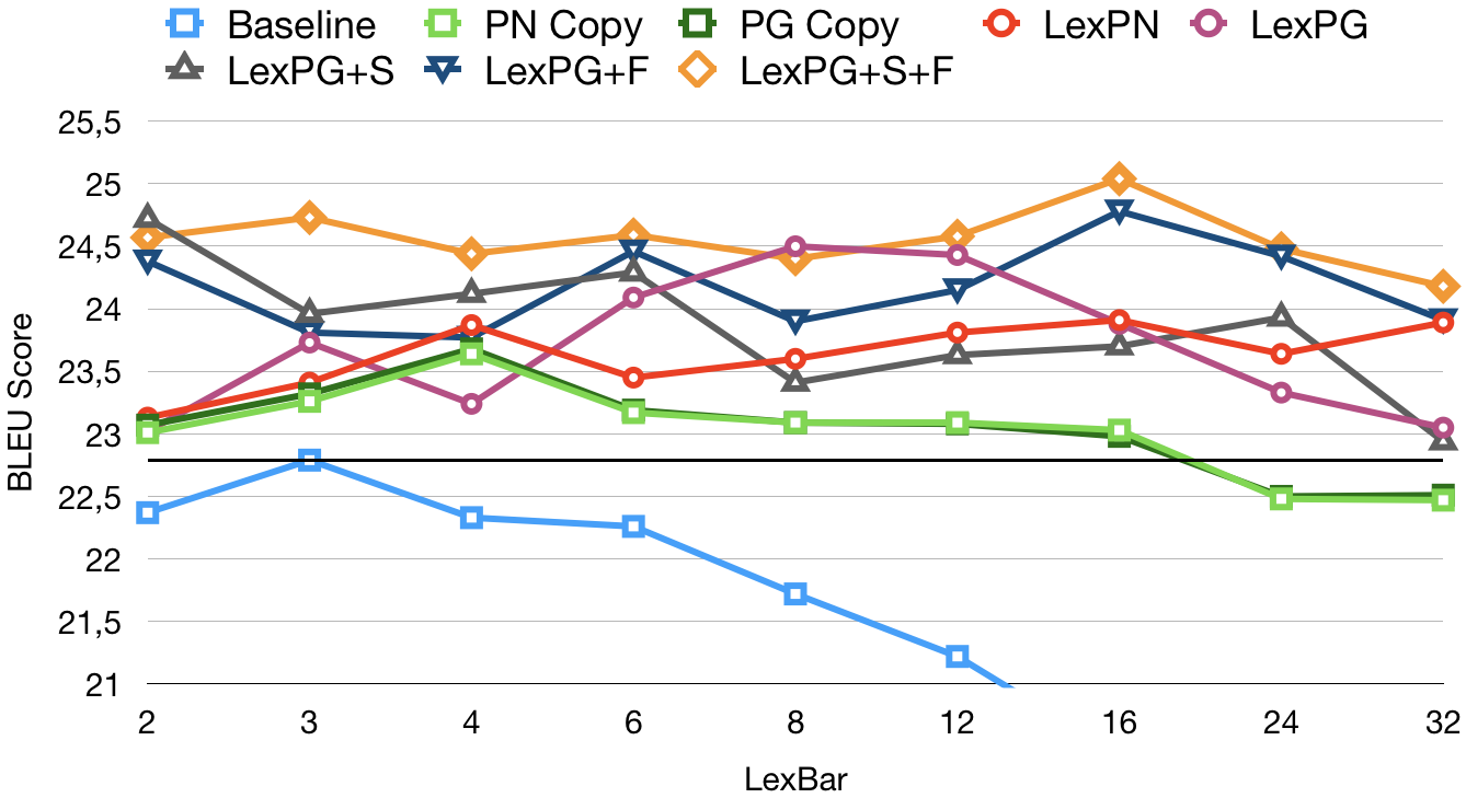
Figure 1: Coverage study: reduce source and target lexicon size.

Among the proposed models, we see that LexPG’s performance is significantly better than the baseline models, but its curve is somewhat unstable. Similar instability was also observed for Russian-English and Czech-English, for which LexPG achieves their best BLEU scores under completely different $\mathrm{LexBar}$ settings. The problem with this is that given any dataset, one might need to perform a lot of parameter search to find an optimal $\mathrm{LexBar}$ for LexPG.

Another interesting observation is that our further analysis shows that the performance of the neural conditional language model component of LexPG (evaluated by removing the dictionary fusion at test time) was able to benefit from LexPG, receiving a slight boost when LexPG reaches its peak at $\mathrm{LexBar}=8$. We suspect that the direct usage of attention $\alpha$ in LexPG’s loss function might have led to this outcome.

LexPG+S has a curve that decreases as $\mathrm{LexBar}$ increases, but at a pace much more subtle than all baselines. Comparing to LexPG, LexPG+S’s $\beta$ layer was able to benefit from the rich neural lexical coverage, although this dependency eventually led to worsened performance as neural lexicon shrinks.

We ran additional tests and found that both LexPG and LexPG+S are much more sensitive to source neural lexicon size than target. This could be caused by the fact that the dictionary fusion for LexPG and LexPG+S is not exposed to whether the source element is covered by the dictionary or not, leaving the pointer generator to learn such coverage on its own. When the neural lexicon is small, LexPG(+S) will not be able to distinguish between different unknown source words, since all UNK have the same word embedding for the neural decoder.

Unlike LexPG(+S), LexPG+F is exposed to dictionary features and is so far the most stable one: having been able to maintain overall better performance even when the neural lexicon is reduced to around 10%. Where LexPG(+S)’s neural decoder may not have enough information to determine the correct responses to source UNKs, LexPG+F’s knowledge of the dictionary is shown to help make better decisions. The conflict between attention $\alpha$ and word alignments are also resolved by the inclusion of a separate alignment $\beta$ score in LexPG+S+F, making it our most stable and well performing model.

Since the performance of our proposed model does not drop and in some cases improves the BLEU scores even with a smaller neural network, we think it may also benefit production scenarios where the number of parameters are tightly constrained (e.g., deployment on mobile devices). In our most extreme case, LexPG’s saved model (neural parameters and pickled encoder-decoder class object with full dictionary) is almost 4 times smaller than a baseline model with 100K (50K for source and 50K for target side) neural dictionary (221M vs 871M). Less neural parameters also leads to faster learning and inference. In our experiments the training of LexPG+S+F model despite its complexity is only 10% slower than a baseline with the same neural lexicon. If we compare against increased LexBar without sacrificing BLEU score, LexPG+F’s training with LexBar=16 is about 3-4 times faster than baseline (LexBar=2).

5.4 Expansion Study: expanding the dictionary post-training

The purpose of this study is to evaluate the dictionary component’s extensibility. We first train the models using the same training data above, then add more entries into the dictionary without changing any of the neural parameters. Theoretically it is possible to use a real bilingual dictionary, but for the sake of simplicity, these additional entries are obtained using word alignment of the test set.

Language pair	DEEN	DEEN+	CSEN	CSEN+	RUEN	RUEN+
Baseline	22.37	-	9.35	-	9.26	-
PN Copy	23.01	-	10.41	-	9.72	-
PG Copy	23.07	-	10.85	-	10.47	-
LexPN	23.08	23.24	10.51	10.99	9.54	10.08
LexPG	23.02	23.70	12.25	13.66	10.67	12.63
LexPG+S	24.72	25.30	11.71	12.79	11.56	13.28
LexPG+F	24.38	25.01	12.05	13.45	11.24	13.02
LexPG+S+F	24.57	25.50	12.49	13.89	12.18	13.58

Table 5: Expansion study: adding more entries into the dictionary post-training. The proposed models are first trained with existing automatically acquired entries, then prior to testing new entries are added to further expand the dictionary.

One might think that such exposure to the test set would give our models unfair advantage, but we argue that this is actually a noisier substitution to a real bilingual dictionary. Our intent here is merely to simplify dictionary collection/generation. Ideally, a bilingual dictionary should contain the aligned components and with better quality as well. What we are doing is essentially adding a flawed fraction of a real bilingual dictionary, to show how well the model can leverage such additional knowledge. During these experiments, the neural conditional language model, its word embedding matrices and other neural components are completely untouched. And as the results show, our proposed models are indeed able to put these information into good use and boost its performance.

To accommodate changes in a pretrained neural translation model, extensive data collection and retraining is usually required for active learning (or even life-long learning). Our use of a bilingual lexicon provides an alternative. The bilingual lexicon can be updated dynamically while keeping the neural model fixed.

5.5 Improving The Bilingual Lexicon

At the beginning of §4 we claim that the dictionary entries we used in our experiments are merely “dictionary-like”. Indeed, word alignment can only produce word-to-word alignments and cannot handle phrases. In some cases, words that should have been aligned to multi-word phrases are only aligned to one of the words in the phrase (e.g. “Bundeskanzler” aligned to “Federal” instead of “Federal Chancellor”). More over, the aligner itself is not exactly error-proof. It is therefore reasonable to assume that there is a significant amount of error which could be humanly corrected in the “dictionary” we used.

Aside from relying on alignment, there are many other potential ways to improve the dictionary, such as through crowd-sourcing and extracting entries from a real bilingual dictionaries. The dictionary itself can also contain word-to-phrase translations, which can be hugely beneficial for languages with a lot of compound words and idioms. Through preprocessing to identify known named entities (e.g. “Monty Python’s Life of Brian”), we may even enforce more constraints on how specific terms should be translated.

6 Conclusions and Future Work

We present several simple and highly practical approaches to incorporating structured symbolic knowledge – a bilingual dictionary – into a standard neural machine translation model. Our experimental results show that these methods not only produce much better results, but are faster to train, smaller in parameter size, and overall more extensible to adding new knowledge.

For the future, we think it is possible to substitute the LSTM-based neural conditional language model with a transformer (Vaswani et al., 2017). Experimenting on pretraining the neural conditional language model and only train the proposed LexPG(+S)(+F) components may also be of interest, as this would further demonstrate the flexibility of our proposed approach.

On a separate track, we would also like to investigate the possibility of leveraging even more structured knowledge, such as a phrase-table. The ability to accommodate complex mapping constraints, including Synchronous Context-Free Grammar (SCFG) is also appealing and worthy of our endeavour.

References

- Arcan et al. (2015) Mihael Arcan, Marco Turchi, and Paul Buitelaar. 2015. Knowledge portability with semantic expansion of ontology labels. In Proceedings of the 53rd Annual Meeting of the Association for Computational Linguistics and the 7th International Joint Conference on Natural Language Processing (Volume 1: Long Papers), pages 708–718, Beijing, China. Association for Computational Linguistics.
- Arthur et al. (2016) Philip Arthur, Graham Neubig, and Satoshi Nakamura. 2016. Incorporating discrete translation lexicons into neural machine translation. In Proceedings of the 2016 Conference on Empirical Methods in Natural Language Processing, pages 1557–1567, Austin, Texas. Association for Computational Linguistics.
- Bahdanau et al. (2014) Dzmitry Bahdanau, Kyunghyun Cho, and Yoshua Bengio. 2014. Neural machine translation by jointly learning to align and translate. CoRR, abs/1409.0473.
- Chatterjee et al. (2017) Rajen Chatterjee, Matteo Negri, Marco Turchi, Marcello Federico, Lucia Specia, and Frédéric Blain. 2017. Guiding neural machine translation decoding with external knowledge. In Proceedings of the Second Conference on Machine Translation, pages 157–168, Copenhagen, Denmark. Association for Computational Linguistics.
- Ghader and Monz (2017) Hamidreza Ghader and Christof Monz. 2017. What does attention in neural machine translation pay attention to? In Proceedings of the Eighth International Joint Conference on Natural Language Processing (Volume 1: Long Papers), pages 30–39, Taipei, Taiwan. Asian Federation of Natural Language Processing.
- Gu et al. (2016) Jiatao Gu, Zhengdong Lu, Hang Li, and Victor O.K. Li. 2016. Incorporating copying mechanism in sequence-to-sequence learning. In Proceedings of the 54th Annual Meeting of the Association for Computational Linguistics (Volume 1: Long Papers), pages 1631–1640. Association for Computational Linguistics.
- Gulcehre et al. (2016) Caglar Gulcehre, Sungjin Ahn, Ramesh Nallapati, Bowen Zhou, and Yoshua Bengio. 2016. Pointing the unknown words. In Proceedings of the 54th Annual Meeting of the Association for Computational Linguistics (Volume 1: Long Papers), pages 140–149, Berlin, Germany. Association for Computational Linguistics.
- Hasler et al. (2018) Eva Hasler, Adrià de Gispert, Gonzalo Iglesias, and Bill Byrne. 2018. Neural machine translation decoding with terminology constraints. In Proceedings of the 2018 Conference of the North American Chapter of the Association for Computational Linguistics: Human Language Technologies, Volume 2 (Short Papers), pages 506–512, New Orleans, Louisiana. Association for Computational Linguistics.
- Hochreiter and Schmidhuber (1997) Sepp Hochreiter and Jürgen Schmidhuber. 1997. Long short-term memory. Neural computation, 9(8):1735–1780.
- Hokamp and Liu (2017) Chris Hokamp and Qun Liu. 2017. Lexically constrained decoding for sequence generation using grid beam search. In Proceedings of the 55th Annual Meeting of the Association for Computational Linguistics (Volume 1: Long Papers), pages 1535–1546, Vancouver, Canada. Association for Computational Linguistics.
- Jean et al. (2015) Sébastien Jean, Kyunghyun Cho, Roland Memisevic, and Yoshua Bengio. 2015. On using very large target vocabulary for neural machine translation. In Proceedings of the 53rd Annual Meeting of the Association for Computational Linguistics and the 7th International Joint Conference on Natural Language Processing (Volume 1: Long Papers), pages 1–10, Beijing, China. Association for Computational Linguistics.
- Kingma and Ba (2015) Diederik P Kingma and Jimmy Ba. 2015. Adam: A method for stochastic optimization. In International Conference on Learning Representations.
- Koehn et al. (2003) Philipp Koehn, Franz Josef Och, and Daniel Marcu. 2003. Statistical phrase-based translation. In Proceedings of the 2003 Conference of the North American Chapter of the Association for Computational Linguistics on Human Language Technology - Volume 1, NAACL ’03, pages 48–54, Stroudsburg, PA, USA. Association for Computational Linguistics.
- Li et al. (2018) Xiaoqing Li, Jinghui Yan, Jiajun Zhang, and Chengqing Zong. 2018. Neural name translation improves neural machine translation. In China Workshop on Machine Translation, pages 93–100. Springer.
- Liang et al. (2006) Percy Liang, Ben Taskar, and Dan Klein. 2006. Alignment by agreement. In Proceedings of the Human Language Technology Conference of the NAACL, Main Conference.
- Luong et al. (2015a) Thang Luong, Hieu Pham, and Christopher D. Manning. 2015a. Effective approaches to attention-based neural machine translation. In Proceedings of the 2015 Conference on Empirical Methods in Natural Language Processing, pages 1412–1421. Association for Computational Linguistics.
- Luong et al. (2015b) Thang Luong, Ilya Sutskever, Quoc Le, Oriol Vinyals, and Wojciech Zaremba. 2015b. Addressing the rare word problem in neural machine translation. In Proceedings of the 53rd Annual Meeting of the Association for Computational Linguistics and the 7th International Joint Conference on Natural Language Processing (Volume 1: Long Papers), pages 11–19, Beijing, China. Association for Computational Linguistics.
- Mi et al. (2016) Haitao Mi, Zhiguo Wang, and Abe Ittycheriah. 2016. Vocabulary manipulation for neural machine translation. In Proceedings of the 54th Annual Meeting of the Association for Computational Linguistics (Volume 2: Short Papers), pages 124–129. Association for Computational Linguistics.
- Neubig et al. (2017) Graham Neubig, Chris Dyer, Yoav Goldberg, Austin Matthews, Waleed Ammar, Antonios Anastasopoulos, Miguel Ballesteros, David Chiang, Daniel Clothiaux, Trevor Cohn, Kevin Duh, Manaal Faruqui, Cynthia Gan, Dan Garrette, Yangfeng Ji, Lingpeng Kong, Adhiguna Kuncoro, Gaurav Kumar, Chaitanya Malaviya, Paul Michel, Yusuke Oda, Matthew Richardson, Naomi Saphra, Swabha Swayamdipta, and Pengcheng Yin. 2017. Dynet: The dynamic neural network toolkit. arXiv preprint arXiv:1701.03980.
- Post and Vilar (2018) Matt Post and David Vilar. 2018. Fast lexically constrained decoding with dynamic beam allocation for neural machine translation. In Proceedings of the 2018 Conference of the North American Chapter of the Association for Computational Linguistics: Human Language Technologies, Volume 1 (Long Papers), pages 1314–1324, New Orleans, Louisiana. Association for Computational Linguistics.
- Sajjad et al. (2017) Hassan Sajjad, Fahim Dalvi, Nadir Durrani, Ahmed Abdelali, Yonatan Belinkov, and Stephan Vogel. 2017. Challenging language-dependent segmentation for Arabic: An application to machine translation and part-of-speech tagging. In Proceedings of the 55th Annual Meeting of the Association for Computational Linguistics (Volume 2: Short Papers), pages 601–607, Vancouver, Canada. Association for Computational Linguistics.
- See et al. (2017) Abigail See, Peter J. Liu, and Christopher D. Manning. 2017. Get to the point: Summarization with pointer-generator networks. In Proceedings of the 55th Annual Meeting of the Association for Computational Linguistics (Volume 1: Long Papers), pages 1073–1083. Association for Computational Linguistics.
- Sennrich et al. (2016) Rico Sennrich, Barry Haddow, and Alexandra Birch. 2016. Neural machine translation of rare words with subword units. In Proceedings of the 54th Annual Meeting of the Association for Computational Linguistics (Volume 1: Long Papers), pages 1715–1725, Berlin, Germany. Association for Computational Linguistics.
- Song et al. (2019) Kai Song, Yue Zhang, Heng Yu, Weihua Luo, Kun Wang, and Min Zhang. 2019. Code-switching for enhancing NMT with pre-specified translation. In Proceedings of the 2019 Conference of the North American Chapter of the Association for Computational Linguistics: Human Language Technologies, Volume 1 (Long and Short Papers), pages 449–459, Minneapolis, Minnesota. Association for Computational Linguistics.
- Sutskever et al. (2014) Ilya Sutskever, Oriol Vinyals, and Quoc V. Le. 2014. Sequence to sequence learning with neural networks. In Proceedings of the 27th International Conference on Neural Information Processing Systems - Volume 2, NIPS’14, pages 3104–3112, Cambridge, MA, USA. MIT Press.
- Vaswani et al. (2017) Ashish Vaswani, Noam Shazeer, Niki Parmar, Jakob Uszkoreit, Llion Jones, Aidan N Gomez, Ł ukasz Kaiser, and Illia Polosukhin. 2017. Attention is all you need. In Advances in Neural Information Processing Systems 30, pages 5998–6008. Curran Associates, Inc.
- Vinyals et al. (2015) Oriol Vinyals, Meire Fortunato, and Navdeep Jaitly. 2015. Pointer networks. In C. Cortes, N. D. Lawrence, D. D. Lee, M. Sugiyama, and R. Garnett, editors, Advances in Neural Information Processing Systems 28, pages 2692–2700. Curran Associates, Inc.
- Wang et al. (2017) Yuguang Wang, Shanbo Cheng, Liyang Jiang, Jiajun Yang, Wei Chen, Muze Li, Lin Shi, Yanfeng Wang, and Hongtao Yang. 2017. Sogou neural machine translation systems for WMT17. In Proceedings of the Second Conference on Machine Translation, pages 410–415, Copenhagen, Denmark. Association for Computational Linguistics.