Abstract

The MiniBooNE collaboration has reported an excess of $460.5\pm 95.8$ electron-like events ($4.8\sigma$). We propose an explanation of these events in terms of a sterile neutrino decaying into a photon and a light neutrino. The sterile neutrino has a mass around 250 MeV and it is produced from kaon decays in the proton beam target via mixing with the muon or the electron in the range $10^{-11}\lesssim|U_{\ell 4}|^{2}\lesssim 10^{-7}$ ($\ell=e,\mu$). The model can be tested by considering the time distribution of the events in MiniBooNE and by looking for single-photon events in running or upcoming neutrino experiments, in particular by the suite of liquid argon detectors in the short-baseline neutrino program at Fermilab.

1 Introduction

The MiniBooNE collaboration has published evidence for an excess of electron-like events of $381.2\pm 85.2$ above their background expectation [1], confirming previous hints present in both, neutrino and anti-neutrino beam modes [2]. The combined excess of $460.5\pm 95.8$ events corresponds to a significance of $4.8\sigma$. The collaboration presents the results in the context of $\overset{\raisebox{-1.49994pt}{\scalebox{0.4}{{(}}}\raisebox{-3.00003pt}{{\hskip 0.29999pt--\hskip 0.50003pt}}\raisebox{-1.49994pt}{\scalebox{0.4}{{)}}}}{\nu}_{\mu}\to\overset{\raisebox{-1.49994pt}{\scalebox{0.4}{{(}}}\raisebox{-3.00003pt}{{\hskip 0.29999pt--\hskip 0.50003pt}}\raisebox{-1.49994pt}{\scalebox{0.4}{{)}}}}{\nu}_{e}$ neutrino oscillations, under the hypothesis of a sterile neutrino with a neutrino mass-squared difference $\Delta m^{2}$ of order 1 eV², motivated by a previous claim from LSND [3]. The interpretation of the above mentioned results in terms of neutrino oscillations with an eV-scale sterile neutrino is in strong conflict with data on $\overset{\raisebox{-1.49994pt}{\scalebox{0.4}{{(}}}\raisebox{-3.00003pt}{{\hskip 0.29999pt--\hskip 0.50003pt}}\raisebox{-1.49994pt}{\scalebox{0.4}{{)}}}}{\nu}_{e}$ and $\overset{\raisebox{-1.49994pt}{\scalebox{0.4}{{(}}}\raisebox{-3.00003pt}{{\hskip 0.29999pt--\hskip 0.50003pt}}\raisebox{-1.49994pt}{\scalebox{0.4}{{)}}}}{\nu}_{\mu}$ neutrino disappearance at the $\Delta m^{2}\sim 1$ eV² scale [4, 5, 6]. This motivates to look for other new-physics explanations, beyond sterile neutrino oscillations.

In this paper we propose a sterile neutrino in the 150 to 300 MeV mass range, which is produced in the beam target from kaon decay via mixing either with electron or muon neutrinos. Subsequently it decays inside the MiniBooNE detector into a photon and a light neutrino. Since the electromagnetic shower of a photon inside MiniBooNE cannot be distinguished from the one of an electron or positron the photon can explain the observed excess events. We study the energy and angular spectra and predict a specific time distribution of the events. In order to obtain a reasonable fit to the angular distribution, we are driven to heavy neutrino masses around 250 MeV, which can be produced by kaon decays in the beam target. For lighter neutrino decays, the signal is too much forward peaked, inconsistent with MiniBooNE data [7]. Then the heavy neutrinos are only moderately relativistic and therefore our signal has a specific time structure, which provides a testable signature of our model [8]. The required parameters are consistent with all laboratory, astrophysics, and cosmology bounds. Current bounds and sensitivities of the upcoming short-baseline program at Fermilab for $N\to\gamma\nu$ with the heavy neutrino $N$ in the relevant mass range have been discussed in ref. [8]. Our model differs from various previously discussed explanations of the MiniBooNE and LSND anomalies based on the decay of a sterile neutrino. In the explanations of refs. [9, 10] and [11, 12] the heavy neutrino is produced by $\nu_{\mu}$ scattering inside the detector and has to decay with a very short lifetime into a photon or an $e^{\pm}$ pair, respectively. The photon model from ref. [10] is by now excluded by searches for radiative neutrino decays from kaons by the ISTRA+ experiment [13], see also [14, 15]. For other decay scenarios and related work see refs. [16, 17, 18, 19, 6].

The article is structured as follows. In section 2 we introduce the model and in section 3 we describe the calculation of the MiniBooNE signal, including the time, energy, and angular event distributions. We present our $\chi^{2}$ fit to the data in section 4. The results are discussed in terms of the model parameters in section 5, which includes also a discussion of other constraints on the model and possible tests in existing or upcoming experiments. In section 6 we conclude. Details of the heavy neutrino flux calculation are given in appendix A, in appendix B we discuss the impact of the timing cut on the MiniBooNE fit result.

2 The model

We consider one heavy Dirac neutrino $N$ with mass $m_{N}$ that mixes with the SM neutrinos, parameterized by the leptonic mixing matrix $U$. The sub-matrix $U_{\ell i}$ with $\ell=e,\mu,\tau$ and $i=1,2,3$ is approximately the PMNS matrix that gives rise to neutrino oscillations, and the matrix elements $U_{\ell 4}$ allow $N$ to interact with the weak currents and the lepton doublets of the Standard Model. Focusing on the case $m_{N}={\cal O}(100)$ MeV, we consider effective four-fermion interactions between the heavy neutrino and the SM particles, which are the mesons and leptons at this energy scale. Of particular importance is the following effective operator:

$${\cal O}_{\ell Nq_{u}q_{d}}=U_{\ell 4}V_{q_{u}q_{d}}\,G_{F}\,\left[\bar{q}_{u}\gamma^{\mu}(1-\gamma_{5})q_{d}\right]\,\left[\bar{\ell}\gamma_{\mu}(1-\gamma_{5})N\right]+\text{h.c.}\,,$$ (1)

where $G_{F}$ is the Fermi constant, $q_{u}$ and $q_{d}$ are up-type and down-type quarks, respectively, $V$ is the CKM matrix, and $\ell$ is a charged lepton. Fixing the CKM matrix element to $V_{us}$, the operator in eq. (1) allows us to calculate the branching ratio of the kaon into a lepton $\ell=e,\mu$ and the neutrino $N$. For later use we define the following quantity:

$$\rho_{\ell}(m_{N}) \equiv\frac{\text{Br}(K\to\ell N)}{\text{Br}(K\to\mu\nu)}$$

$$=\frac{\text{Br}(K\to\ell\nu)}{\text{Br}(K\to\mu\nu)}\,|U_{\ell 4}|^{2}\,\frac{\left(x_{N}^{2}+x_{\ell}^{2}-(x_{N}^{2}-x_{\ell}^{2})^{2}\right)\sqrt{(1-(x_{N}+x_{\ell})^{2})(1-(x_{N}-x_{\ell})^{2})}}{x_{\ell}^{2}(1-x_{\ell}^{2})^{2}}\,,$$ (2)

which takes into account the mixing of the heavy neutrino and the kinematical factors related to the finite mass of the neutrino [20]. Here, $x_{i}=m_{i}/m_{K}$ and we use Br$(K\to\mu\nu)=0.636$ and Br$(K\to e\nu)=1.6\times 10^{-5}$. The factor $\rho_{\ell}(m_{N})$ is normalized to the branching ratio of $K\to\mu\nu$, since we use the kaon induced $\overset{\raisebox{-1.49994pt}{\scalebox{0.4}{{(}}}\raisebox{-3.00003pt}{{\hskip 0.29999pt--\hskip 0.50003pt}}\raisebox{-1.49994pt}{\scalebox{0.4}{{)}}}}{\nu}_{\mu}$ flux in MiniBooNE to derive the heavy neutrino flux in both cases, $K\to N\mu$ and $K\to Ne$, see appendix A.

In order to obtain the decay $N\to\nu\gamma$ into a light neutrino and a photon we introduce another effective operator to parameterize the possible interaction of $N$ with a photon and light neutrinos via its magnetic moment [9, 21] :

$${\cal O}_{N\nu\gamma}=\frac{1}{\Lambda}\bar{N}\sigma^{\alpha\beta}\nu F_{\alpha\beta}\,,$$ (3)

with the electromagnetic field strength tensor $F_{\mu\nu}=\partial_{\mu}A_{\nu}-\partial_{\nu}A_{\mu}$, the anti-symmetric tensor $\sigma^{\mu\nu}=\gamma^{\mu}\gamma^{\nu}-\gamma^{\nu}\gamma^{\mu}$, and the unknown energy scale $\Lambda$. The operator ${\cal O}_{N\nu\gamma}$ could be created at the loop level, for instance, such that we expect $1/\Lambda$ to be a combination of an inverse mass, unknown coupling constants, and a typical loop suppression factor. The operator in eq. (3) allows $N$ to decay via the process $N\to\nu\gamma$, with the total width in the rest frame of $N$ given by

$$\Gamma_{N\to\nu\gamma}=\frac{m_{N}^{3}}{4\pi\Lambda^{2}}\approx 1.2\times 10^{-16}\,{\rm MeV}\left(\frac{10^{5}\,{\rm TeV}}{\Lambda}\right)^{2}\left(\frac{m_{N}}{250\,{\rm MeV}}\right)^{3}\,.$$ (4)

To predict the energy and angular event spectra in MiniBooNE, we will need the differential decay rates with respect to the photon momentum $p_{\gamma}$ and the angle $\theta$ between the photon and $N$ momenta in the laboratory frame:

$$\frac{d\Gamma_{N\to\nu\gamma}^{\rm lab}}{dp_{\gamma}} =\frac{1}{4\pi\Lambda^{2}}\frac{m_{N}^{4}}{E_{N}p_{N}}\,,$$ (5)

$$\frac{d\Gamma_{N\to\nu\gamma}^{\rm lab}}{d\cos\theta} =\frac{1}{8\pi\Lambda^{2}E_{N}}\frac{m_{N}^{6}}{(E_{N}-p_{N}\cos\theta)^{2}}\,.$$ (6)

The minimum value of $p_{\gamma}$ is in backward direction, $p_{\gamma,\rm min}=(E_{N}-p_{N})/2$, and the maximum value in forward direction, $p_{\gamma,\rm max}=(E_{N}+p_{N})/2$.

The phenomenology of the magnetic moment operator from eq. (3) has been studied extensively in ref. [15], see also [8, 24, 25] for recent considerations. In general this operator provides also a production channel for the heavy neutrinos [14, 15]. Comparing with the results of ref. [15] we will see that for decay rates relevant for our scenario, the production via mixing and weak boson mediated kaon decay as described in relation to eq. (2) will be the dominant production mechanism.

The neutrino mixing parameters $U_{\ell 4}$ allow for various decay modes of $N$ into SM particles via weak boson exchange; depending on its mass into a number of leptons, or also into a lepton and one or more mesons, which have been computed e.g. in refs. [26, 27]. In the mass range of interest to us, $m_{\pi}<m_{N}<m_{K}$, the dominant decay modes are $N\to\ell^{\pm}\pi^{\mp}$ and $N\to\nu\pi^{0}$. Using the results of ref. [27] the decay rate can be estimated by

$$\Gamma_{\pi}\equiv\Gamma_{N\to{\rm lept}\pi} =\frac{G_{F}^{2}f_{h}^{2}m_{N}^{3}}{32\pi}|U_{\ell 4}|^{2}g(m_{\pi},m_{\rm lept},m_{N})$$

$$\approx 3\times 10^{-13}\,{\rm MeV}\,|U_{\ell 4}|^{2}\left(\frac{m_{N}}{250\,{\rm MeV}}\right)^{3}g(m_{\pi},m_{\rm lept},m_{N})\,.$$ (7)

Here, $g(m_{\pi},m_{\rm lept},m_{N})$ is a dimensionless kinematical function depending on the decay channel [27], ”lept” indicates either a light neutrino or a charged lepton of flavour $\ell=e,\mu$, and $f_{h}\approx 130$ MeV is the pion decay constant. As we will see below, for large portions of the parameter space for $\Gamma_{N\to\nu\gamma}$ and $U_{\ell 4}$ required to explain the MiniBooNE events, the decays $N\to{\rm lept}\pi$ will be sub-leading compared to $N\to\nu\gamma$.

Note that a decay width of the scale indicated in eq. (4) corresponds to lifetimes much shorter than milliseconds, and therefore our sterile neutrino decays well before Big Bang nucleo-synthesis and hence does not affect cosmology. Heavy neutrinos in the 100 MeV mass range are at the border of being relevant for supernova cooling arguments. Limits from supernova 1987A on heavy neutrino mixing are avoided in our scenario [28], while the limits due to the magnetic moment operator derived in ref. [15] will be relevant in part of the parameter space able to explain the MiniBooNE excess, see also [29, 30].

To summarize, the relevant phenomenology of our model is determined by three independent parameters, which we chose to be the heavy neutrino mass: $m_{N}$, the mixing with the $e$ or $\mu$ flavour: $|U_{\ell 4}|^{2}$, and the decay width into the photon: $\Gamma_{N\to\nu\gamma}$. We will present the parameter space where the MiniBooNE excess can be explained in terms of those three parameters in section 5 below.

3 The MiniBooNE excess events

Our analysis proceeds as follows: first we construct the kaon flux at the BNB from the given flux of the muon neutrinos. From the kaon flux we derive the flux of the heavy neutrinos and work out its time structure. Then we calculate the energy and angular spectra of the photon from the heavy neutrino decays inside the detector and inside the time window defined by the MiniBooNE collaboration.

In order to calculate the flux of heavy neutrinos $\Phi_{N}(p_{N})$ we proceed as follows. We depart from the kaon contribution to the $\overset{\raisebox{-1.49994pt}{\scalebox{0.4}{{(}}}\raisebox{-3.00003pt}{{\hskip 0.29999pt--\hskip 0.50003pt}}\raisebox{-1.49994pt}{\scalebox{0.4}{{)}}}}{\nu}_{\mu}$ fluxes provided by the MiniBooNE collaboration ref. [31]. Assuming that this flux is dominated by the two-body decay $K\to\nu\mu$ we reconstruct the initial kaon flux, from which in turn we can calculate the heavy neutrino flux at MiniBooNE by taking into account the modified angular acceptance of the detector due to the non-negligible effect of the heavy neutrino mass on the angular distribution. Details of this procedure are provided in appendix A. Note that the flux $\Phi_{N}(p_{N})$ obtained in this way depends on the mass of the heavy neutrino, which we keep implicit to simplify notation.

3.1 Time spectrum

A heavy neutrino with momentum $p_{N}$ arrives at the detector at distance $L$ after a time

$$t_{N}=\frac{t_{0}}{\beta}\,,\qquad\text{with}\qquad t_{0}=\frac{L}{c}\qquad\text{and}\qquad\beta=\frac{p_{N}}{E_{N}}\,,$$ (8)

with the MiniBooNE baseline $L\simeq 540$ m. The ultra-relativistic light neutrinos all arrive after $t_{0}\simeq 1.8\,\mu$s, the heavy neutrinos generally arrive later. In order to calculate the time distribution of the events, we first convert the neutrino flux $\Phi_{N}(p_{N})$ into a function of time,

$$\Phi(t)=\Phi_{N}(p_{N})\left|\frac{dp_{N}}{dt}\right|$$ (9)

with the Jacobian $|dp_{N}/dt|=p_{N}t/(t^{2}-t_{0}^{2})$, which follows form eq. (8). In the decay model, an additional momentum dependence appears due to the effect of the Lorentz boost on the decay rate, which leads to a factor $m_{N}/p_{N}$, see eq. (15) below. Finally, to construct the time spectrum we need to include the time structure of the proton beam, which we approximate with a step-function being non-zero from $t=0$ to $t=\delta t=1.6\,\mu$s [32]. Therefore, we obtain the time spectrum $T(t)$ in the following way:

$$T(t)=\frac{1}{\delta t}\int_{t-\delta t}^{t}dt^{\prime}\Phi(t^{\prime})\frac{m_{N}}{p_{N}(t^{\prime})}\,.$$ (10)

We show the time distribution of the decay events inside the detector for a typical heavy neutrino mass in fig. 1. The contribution of the monochromatic peak from the stopped kaon decays is visible in the discontinuous part of the red curve around $t=3\,\mu$s. It is important to notice, that the neutrino appearance analysis from MiniBooNE considers only events that occur between $t_{0}$ and $t_{0}+1.6\,\mu$s after each beam spill [33]. The fraction of our heavy neutrino signal inside the analysis window is denoted in blue in the figure, those that arrive after $t_{0}+\delta t$ are too late to be included and are denoted in red. The fraction of the events inside the timing window is 41% (34%) in the neutrino (antineutrino) mode. Therefore, we predict a significant fraction of delayed events. Those could be searched for in the MiniBooNE data. Note that MiniBooNE records events within a time window of about 19.8 $\mu$s around each beam spill (cf. ref. [32]). A detailed investigation of events in this time region can be a definite test of our model. Using timing information to test heavy neutrino decays has been suggested previously in ref. [8].

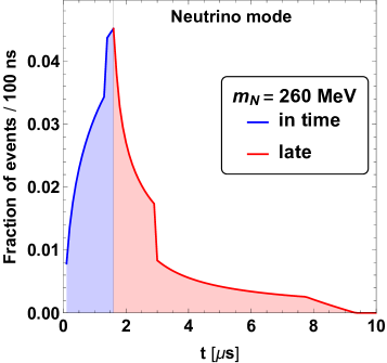
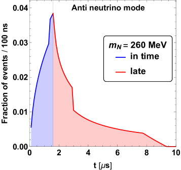
Figure 1: Time distribution of signal events for a sterile neutrino mass of 260 MeV in the neutrino (left) and antineutrino (right) beam mode. For the proton beam we assume a step-function of 1.6 $\mu$s duration. The zero of the time axis corresponds to the time when a neutrino produced at the onset of the beam traveling at the speed of light would arrive at the detector. The blue shaded region indicates the time window used for the analysis (1.6 $\mu$s); it contains 41% (34%) of all events in the neutrino (antineutrino) mode.

3.2 Event numbers, energy and angular spectra

The number of heavy neutrinos that decay inside the detector are obtained by integrating over the heavy neutrino flux $\phi_{N}$, together with the probability $P_{\rm dec}$ that the long lived particles decay within its fiducial volume. Furthermore, a detection efficiency $\epsilon$ has to be included that is an empirical function of the signal energy, here approximated with the momentum of the photon, and the decays have to occur inside a timing window as discussed above. These considerations are summed up in the following master formula:

$$N_{\rm decay}= {\rm POT}\,\rho_{\ell}(m_{N})\,{\rm Br}_{\nu\gamma}\,A_{\rm MB}\int dp_{N}\,\phi_{N}(p_{N})\hat{\epsilon}(p_{N})P_{\rm dec}(p_{N})w_{\rm time}(p_{N},m_{N})\,.$$ (11)

Here, POT denotes the number of protons on target, which is $12.84\,(11.27)\times 10^{20}$ for the neutrino (antineutrino) mode. The factor $\rho_{\ell}(m_{N})$ has been defined in eq. (2) and it includes the mixing matrix element $|U_{\ell 4}|^{2}$ and the branching ratio of the kaon decays into heavy neutrinos. Br${}_{\nu\gamma}=\Gamma_{N\to\nu\gamma}/\Gamma_{\rm tot}$ is the branching ratio for the decay $N\to\nu\gamma$, with $\Gamma_{\rm tot}$ being the total decay width of $N$. In the relevant mass range we have $\Gamma_{\rm tot}\approx\Gamma_{N\to\nu\gamma}+\Gamma_{\pi}$ with $\Gamma_{\pi}$ given in eq. (7). Furthermore, $A_{\rm MB}=\pi(5\,{\rm m})^{2}$ is the effective area of the MiniBooNE detector, and

$$\hat{\epsilon}(p_{N})=\int_{p_{\gamma,\rm min}}^{p_{\gamma,\rm max}}dp_{\gamma}\epsilon(p_{\gamma})\frac{1}{\Gamma_{N\to\nu\gamma}^{\rm lab}}\frac{d\Gamma_{N\to\nu\gamma}^{\rm lab}}{dp_{\gamma}}$$ (12)

is the MiniBooNE detection efficiency [33] $\epsilon(p_{\gamma})$ averaged over the photon momentum distribution for a given $p_{N}$. $P_{\rm dec}$ is the probability that the heavy neutrino decays inside the detector, and $w_{\rm time}$ is a timing-related weight. Using the heavy neutrino arrival time $t_{N}$ from eq. (8) the latter is given by

$$w_{\rm time}(p_{N},m_{N})=\left\{\begin{array}[]{ll}\frac{t_{0}+\delta t-t_{N}}{\delta t}&\text{for }t_{N}<\delta t+t_{0}\\ 0&\text{for }t_{N}\geq\delta t+t_{0}\,.\end{array}\right.$$ (13)

For the decay probability we have

$$P_{\rm dec}(p_{N}) =e^{-L_{1}\Gamma_{\rm tot}\frac{m_{N}}{p_{N}}}-e^{-L_{2}\Gamma_{\rm tot}\frac{m_{N}}{p_{N}}}$$ (14)

$$\approx\Gamma_{\rm tot}\frac{m_{N}}{p_{N}}\Delta L\,,$$ (15)

where $L_{1},L_{2}$ denote the distance of the front and back ends of the detector from the beam production and we assume an effective value of $\Delta L\equiv L_{2}-L_{1}=8$ m. Here $\Gamma_{\rm tot}$ is the heavy neutrino width in the rest frame, a factor $m_{N}/E_{N}$ takes into account the boost into the lab frame of the detector, and $L_{i}\times E_{N}/p_{N}$ is the time the neutrino needs to reach the position $L_{i}$. In eq. (15) we have used an approximation, which holds for the MiniBooNE baseline of $L\approx 540$ m when $\Gamma_{\rm tot}\lesssim 10^{-15}$ MeV. In this approximation the number of events is proportional to $|U_{\ell 4}|^{2}{\rm Br}_{\nu\gamma}\Gamma_{\rm tot}=|U_{\ell 4}|^{2}\Gamma_{N\to\nu\gamma}$.

We remark that in order to fit the observed shapes of the angular and energy spectra, in principle we have to recast the energy of the photon-induced Cherenkov shower (here assumed to be identical to the momentum of the photon from the heavy neutrino decay) into the energy of a light neutrino, $E_{\nu}$, assuming a quasi-elastic scattering event. It turns out, however, that this recasting yields a relative difference on the percent level, such that we will keep the photon energy as our proxy for the reconstructed neutrino energy in the following, for simplicity.

Using the linear approximation for the decay probability (15), and the differential decay widths from eqs. (5) and (6), we construct the predicted angular spectrum ${\cal A}(z)$ with $z\equiv\cos\theta$ and energy spectrum ${\cal E}(E_{\nu})$ in the following way:

$${\cal A}(z)= {\rm POT}\,\rho_{\ell}(m_{N})\,A_{\rm MB}\Delta L\int dp_{N}\Phi_{N}(p_{N})\frac{E_{N}}{p_{N}}w_{\rm time}(p_{N},m_{N})\frac{d\Gamma^{\rm lab}_{N\to\nu\gamma}}{dz}\epsilon(p_{\gamma}(z))\,,$$ (16)

$${\cal E}(p_{\gamma})= {\rm POT}\,\rho_{\ell}(m_{N})\,A_{\rm MB}\Delta L\int dp_{N}\Phi_{N}(p_{N})\frac{E_{N}}{p_{N}}w_{\rm time}(p_{N},m_{N})\frac{d\Gamma^{\rm lab}_{N\to\nu\gamma}}{dp_{\gamma}}\epsilon(p_{\gamma})\,,$$ (17)

where the neutrino flux depends on the horn mode and includes forward and backward decays of the parent meson. The photon momentum is related to the scattering angle by

$$p_{\gamma}(z)=\frac{m_{N}^{2}}{2(E_{N}-p_{N}\cos\theta)}\,.$$ (18)

In our model the ratio of signal events for the two horn polarisations ($R_{\rm pred}$) is determined from the corresponding fluxes, and can be calculated from eq. (11) for a given heavy neutrino mass. We show $R_{\rm pred}$ as a function of $m_{N}$ in fig. 2 for the heavy neutrino being produced together with a muon. The ratio is almost identical when the heavy neutrino is produced together with an electron, aside from the fact that larger values for $m_{N}$ are kinematically accessible.

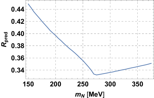
Figure 2: Predicted ratio of heavy neutrino events in the MiniBooNE detector for the horn being in antineutrino mode to the one in neutrino mode as a function of the heavy neutrino mass.

4 Fit to the data

In order to test our model we perform a fit to both, the angular and energy spectra. The data and the different background contributions are read from fig. 14 of ref. [1]. Ideally one would fit the angular and energy information simultaneously by using the 2-dimensional distribution of the data. Unfortunately this information is not available, and therefore we have to fit the energy and angular spectra separately and check if results are consistent. In each case the fit is done fitting simultaneously both the neutrino and anti-neutrino spectra.

Using the results of the previous section, we parameterize our model with two effective parameters, which we chose to be $N_{\rm total}$ and the sterile neutrino mass $m_{N}$. The predicted number of events in a given bin $i$ of the energy or angular data is given by $N_{\nu}f_{i}^{\nu}(m_{N})$ and $N_{\bar{\nu}}f_{i}^{\bar{\nu}}(m_{N})$ for the neutrino and anti-neutrino polarization, respectively. Here,

$$N_{\nu}=\frac{N_{\rm total}}{1+R_{\rm pred}(m_{N})}\,,\qquad N_{\bar{\nu}}=N_{\rm total}\frac{R_{\rm pred}(m_{N})}{1+R_{\rm pred}(m_{N})}\,,$$ (19)

where $R_{\rm pred}(m_{N})$ is the predicted ratio of events in the neutrino and anti-neutrino modes shown in fig. 2, and $f_{i}^{\nu}(m_{N})$, $f_{i}^{\bar{\nu}}(m_{N})$ are the predicted relative contributions for each bin, normalized to 1. They are derived from the corresponding differential spectra given in eqs. (16) and (17).

Bkg contribution	$\nu$ mode	$\bar{\nu}$ mode
$\nu_{e}$ from $\mu$	0.24	0.3
$\nu_{e}$ from $K^{\pm}$	0.22	0.21
$\nu_{e}$ from $K^{0}$	0.38	0.35
$\pi^{0}$ miss	0.13	0.10
$\Delta\to N\gamma$	0.14	0.16
dirt	0.25	0.25
other	0.25	0.25

Table 1: Relative uncertainties $\sigma_{a}$ and $\bar{\sigma}_{a}$ for the various background components, taken from table 1 of ref. [1]. Uncertainties for ’dirt’ and ’other’ are estimates. All background uncertainties are assumed to be uncorrelated.

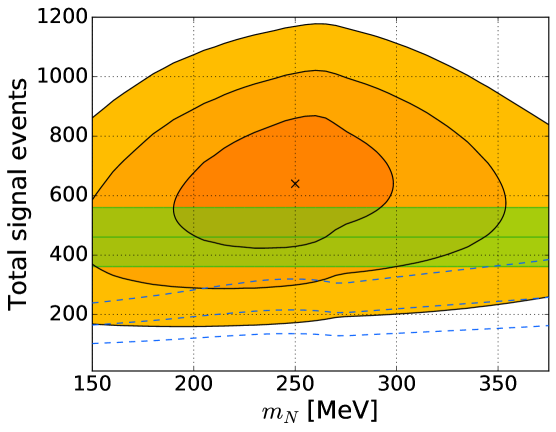
Figure 3: Allowed regions at 1, 2, and 3$\sigma$ for the energy (orange regions) and angular (dashed blue curves) in the $N_{\rm total}$ versus $m_{N}$ parameter space. The best fit of the energy spectral fit is indicated with a cross. The angular fit provides an upper limit on $N_{\rm total}$. In green we show the measured excess of events and its 1$\sigma$ uncertainty. We assume here heavy neutrino mixing with the muon; results for the electron are very similar.

We define the following $\chi^{2}$-function to perform the analysis:

$$\chi^{2}(N_{\nu},m_{N}) = \sum_{i}\frac{\left(O_{i}^{\nu}-b_{a}B_{i}^{a}-N_{\nu}f_{i}^{\nu}(m_{N})\right)^{2}}{(\sigma_{i}^{\rm stat})^{2}+(\sigma_{i}^{\rm syst})^{2}}$$ (20)

$$+\sum_{i}\frac{\left(O^{\bar{\nu}_{i}}-\bar{b}_{a}\bar{B}^{a}_{i}-R_{\rm pred}N_{\nu}f_{i}^{\bar{\nu}}(m_{N})\right)^{2}}{(\bar{\sigma}_{i}^{\rm stat})^{2}+(\bar{\sigma}_{i}^{\rm syst})^{2}}$$

$$+\sum_{a}\left(\frac{b_{a}-1}{\sigma_{a}}\right)^{2}+\sum_{a}\left(\frac{\bar{b}_{a}-1}{\bar{\sigma}_{a}}\right)^{2}\,.$$

Here $i$ labels the angular or energy bins, $a$ labels the background contributions (sum over $a$ is implicit), $O^{\nu}_{i}$ and $O^{\bar{\nu}}_{i}$ are the number of events in each bin $i$ for the $\nu$ and $\bar{\nu}$ mode respectively. $B^{a}_{i}$ and $\bar{B}^{a}_{i}$ are the different $a$ background contributions in each bin $i$, $b_{a}$ and $\bar{b}_{a}$ are the pull parameters that account for their uncertainty $\sigma_{a}$ and $\bar{\sigma}_{a}$, which are taken from table 1 of ref. [1], see Tab. 1. Possible correlations are not taken into account. Furthermore, a totally uncorrelated systematic uncertainty of 20% is considered in each bin to account for possible spectral shape uncertainties: $\sigma^{\rm syst}_{i}(N,m_{N})=0.2N_{\nu}f^{\nu}_{i}(m_{N})$ and $\bar{\sigma}^{\rm syst}_{i}(N,m_{N})=0.2N_{\bar{\nu}}f^{\bar{\nu}}_{i}(m_{N})$.

The results of the angular and energy analyses are shown in figure 3. To be specific, we assume the production mode $K\to N\mu$, results for $K\to Ne$ are very similar. The energy spectrum provides a best fit point at $m_{N}=250$ MeV and $N_{\rm total}=640$ with closed allowed regions. At 68% confidence level our fit allows the masses to vary between 190 MeV and 295 MeV and normalisations between 425 and 865 events, consistent within 1$\sigma$ with the observed number of excess events $N_{\rm obs}=460.5\pm 95.8$, as indicated by the green band in the plot. Note that this comparison is only indicative, since the data used in our fit (taken from fig. 14 of ref. [1]) uses a lower energy threshold and therefore the number of excess events is somewhat larger, consistent with our best fit value. The best fit point has $\chi^{2}_{\rm min}/{\rm dof}=58.1/36$ which corresponds to a $p$ value of about 1% (see discussion below). In contrast, the angular spectrum only provides an upper bound on $N_{\rm total}$ which is in some tension with the energy fit.

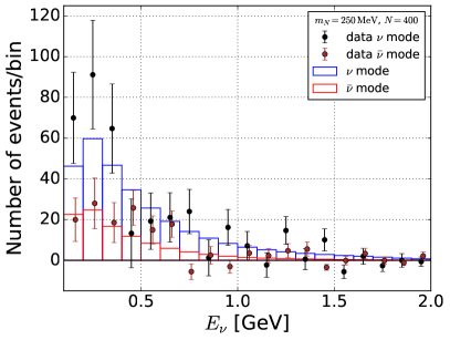
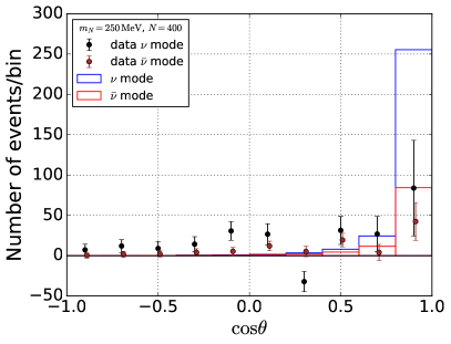
Figure 4: Predicted energy (left) and angular (right) spectra for $m_{N}=250\,{\rm MeV}$ and $N_{\rm total}=400$. The dots are the data with background subtracted, where each background component is re-scaled by the corresponding pull parameter obtained from the fit. Error bars include statistical and systematical errors.

In order to investigate the quality of the fit we show in figure 4 the predicted energy and angular spectra for $m_{N}=250$ MeV and $N_{\rm total}$ fixed to 400, chosen within the 1$\sigma$ range of the observed value. From the left panel we see that our model explains well the excess events in the energy spectrum. A significant contribution to the $\chi^{2}$ comes from bins above 1 GeV, where a signal is neither observed nor predicted. This explains the rather low $p$-value of only 1%. The right panel shows that the angular shape for the anti-neutrino mode is in good agreement with the observations, while the signal is somewhat too much forward peaked in the neutrino mode. From comparing the neutrino-mode spectra in the two panels (blue histograms), the tension between energy and angular fit is apparent. While the energy spectrum would prefer to increase the normalization, this would clearly worsen the prediction in the forward angular bin. Note however, that the largest contribution to the angular $\chi^{2}$ comes from the three bins around $\cos\theta=0$, including the one with the downward fluctuation. Those bins are difficult to explain by any smooth function.

A general discussion of the angular event distribution in decay models can be found in ref. [7]. We stress that to definitely assess the viability of our model a joint energy and angular fit should be performed, including detailed acceptances and efficiencies suitable to our signature. Let us also mention that both the timing cut and the implementation of the angular acceptance is important to predict the angular shape, since both affect mostly the signal from the decay of “slow” neutrinos, which give the main contribution to events with $\cos\theta<1$. In appendix B we show the fit results without imposing the 1.6$\mu$s timing cut, which leads to an improved angular fit. Below we proceed under the assumption that our model does provide an acceptable fit to MiniBooNE data.

5 Discussion of results

5.1 Available parameter space of the model

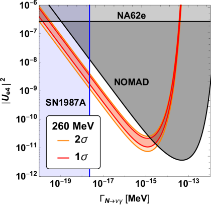
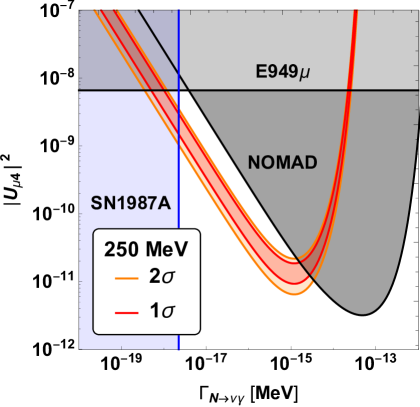
Figure 5: Parameter region in the plane of $\Gamma_{N\to\nu\gamma}$ and $|U_{\ell 4}|^{2}$ that is consistent with the observed MiniBooNE excess at 1 and 2$\sigma$ for the neutrino mass fixed at the best fit point. The left (right) plot assumes that $N$ is produced from a kaon decay with an associated electron (muon) and corresponds to $m_{N}=260\,(250)$ MeV. Also shown are upper limits on $|U_{\ell 4}|^{2}$ from NA62 [34] and E949 [35] and the region excluded by NOMAD from the search in ref. [36], interpreted in our model, as well as the region for $\Gamma_{N\to\nu\gamma}$ disfavoured by SN1987A [15].

By using eq. (11), the total number of events determined by the fit above can be translated into the parameter space given by the neutrino mixing parameter $|U_{\ell 4}|^{2}$ and the heavy neutrino decay rate $\Gamma_{N\to\nu\gamma}$. In fig. 5 we show the 1 and $2\sigma$ contours for those two parameters for the neutrino mass fixed at the best fit point. The straight part on the left side corresponds to the linear approximation for the decay probability, eq. (15), where event numbers are proportional to the product $|U_{\ell 4}|^{2}\Gamma_{N\to\nu\gamma}$. The linear approximation breaks down when the decay length becomes shorter than the MiniBooNE baseline and most of the neutrinos decay before reaching the detector. This leads to the upturn of the allowed region visible in the plots for decay rates $\Gamma_{N\to\nu\gamma}\gtrsim 10^{-15}$ MeV. This value depends only weakly on $m_{N}$ and defines a minimum value of $|U_{\ell 4}|^{2}$ needed to explain the excess of roughly $2\times 10^{-11}$. The lower limit on $|U_{\ell 4}|^{2}$ is shown as a function of the heavy neutrino mass in fig. 6. The dark and light orange shaded regions correspond to the 1$\sigma$ and 2$\sigma$ range for $m_{N}$ as shown in fig. 3. Note that we do not consider masses below 150 MeV in order to avoid $N$ production due to pion decays. We see that the excess can be explained by a wide range of values for the mixing and for the decay rate. Let us now consider other constraints on those parameters.

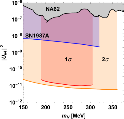
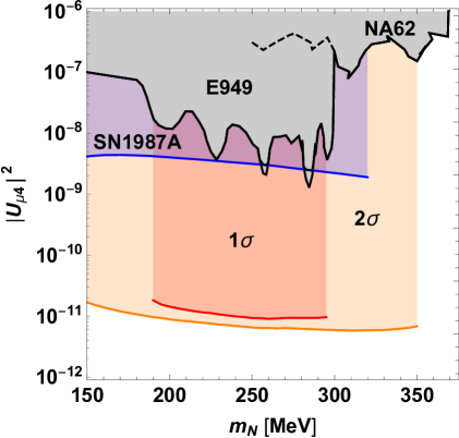
Figure 6: Parameter region in the plane of $m_{N}$ and $|U_{\ell 4}|^{2}$ that is consistent with the observed MiniBooNE excess at 1 and 2$\sigma$. For each point in the allowed region the decay rate $\Gamma_{N\to\nu\gamma}$ can be chosen such that the observed MiniBooNE events can be obtained. For the left (right) panel the heavy neutrino is produced by $K\to eN\,(\mu N)$. Excluded parameter space from peak searches in the kaon decay spectra of electron and muon from the NA62 [34] and E949 experiments [35] is shown as gray shaded regions. The regions disfavoured by SN1987A constraints on $\Gamma_{N\to\nu\gamma}$ [15] are shown as blue shaded regions.

NOMAD:

The single photon signature predicted in our model can be searched for in various other neutrino experiments. A rather sensitive search comes from the NOMAD experiment at CERN. An overview of the experiment is given in ref. [37]. An analysis searching for single photon events (motivated by the MiniBooNE observation) yields 78 observed events in forward direction versus $76.6\pm 4.9\pm 1.9$ expected, which was interpreted as a null result and an upper bound of 18 events at 90% CL has been set on single photon events [36]. We can interpret this bound as a limit within our model. We use the kaon-produced muon neutrino flux from ref. [38] and construct the heavy neutrino flux as described in appendix A. The number of heavy neutrino decays in the detector is estimated as in eq. (11). The POT is $2.2\times 10^{19}$ and we use a constant reconstruction efficiency of 90%, an analysis efficiency of 8%, and a trigger efficiency of 30% [36]. In order to take into account an analysis cut on the observed energy we consider only heavy neutrinos with momentum greater than 1.5 GeV. We do not apply any time window for the events.

The parameter space excluded by NOMAD by requiring that less than 18 events are predicted is shown as the dark gray shaded region in fig. 5. Since the baseline of NOMAD is shorter than MiniBooNE and the neutrino energies are higher, the decay rate for which neutrinos start decaying before reaching the detector is shifted to higher values of $\Gamma_{N\to\nu\gamma}$ for NOMAD compared to MiniBooNE and NOMAD excludes the “non-linear” part of the parameter space. In the linear regime for the decay probability the NOMAD bound is always consistent with the value $|U_{\ell 4}|^{2}\Gamma_{N\to\nu\gamma}$ required to explain MiniBooNE. We have checked that the predicted number of events in NOMAD is about $5.4\times 10^{-3}$ times the signal events in MiniBooNE, with very little dependence of this number on $m_{N}$ within the interesting range. Therefore, the NOMAD bound limits the available parameter space to the linear regime but does not provide a further constraint on the range of the parameters.

Limits from kaon experiments.

Due to the long lifetimes of the heavy neutrinos the vast majority of the produced $N$ decay outside the detectors in most kaon experiments. However, an observable feature of their presence is given by an additional peak in the spectrum of the lepton from the decaying kaon. The NA62 experiment has recently published a search for heavy neutral leptons that are produced in kaon decays. Not observing candidates for kaon decays into heavy neutrinos, they placed upper limits at the 90% CL of around $|U_{\ell 4}|^{2}\sim 10^{-7}$ for $\ell=e,\mu$ and heavy neutral leptons with masses between 170 and 448 MeV for $\ell=e$ and between 250 and 373 MeV for $\ell=\mu$ [34]. Earlier searches for heavy neutrinos from the E949 experiment studied the muon spectra from about $10^{12}$ stopped kaon decays. In their analysis, the collaboration derived the still most stringent upper limits at the 90% CL on $|U_{\mu 4}|^{2}$ down to $10^{-9}$ for heavy neutrinos with masses between 175 and 300 MeV [35]. We show the region excluded by E949 and NA62 in figs. 5 and 6 as a gray area.

To summarize sofar, as visible in fig. 6, several orders of magnitude in mixing are available to explain the MiniBooNE excess in this model. For a fixed value of $m_{N}$, for each value of $|U_{\ell 4}|^{2}$ in the allowed range, the value of the decay rate can be adjusted such that the event numbers are kept constant. Requiring $N_{\rm total}=400$ events in MiniBooNE we have approximately

$$\Gamma_{N\to\nu\gamma}\simeq 3\times 10^{-17}\,{\rm MeV}\left(\frac{10^{-10}}{|U_{\ell 4}|^{2}}\right)\left(\frac{250\,{\rm MeV}}{m_{N}}\right)^{2.3}\left(\frac{N_{\rm total}}{400}\right)\,,$$ (21)

where we have used the linear approximation for the decay probability and the fact that then event numbers are proportional to the product $|U_{\ell 4}|^{2}\Gamma_{N\to\nu\gamma}$. The power of the mass dependence has been obtained by fitting the numerical result with a power law and it is rather accurate in the range $150\,{\rm MeV}<m_{N}<300\,{\rm MeV}$.

Constraint from SN1987A.

As discussed in ref. [15], a heavy neutrino interacting via the operator (3) may contribute to the cooling rate of a supernova. In order to be consistent with the neutrino observation of SN1987A, too fast cooling has to be avoided. This argument can be used to disfavour certain regions in the parameter space of $m_{N}$ and $\Gamma_{N\to\nu\gamma}$. In the parameter region of our interest those considerations lead to a lower bound on the decay rate of approximately [15]

$$\Gamma_{N\to\nu\gamma}>2.4\times 10^{-18}\,{\rm MeV}\left(\frac{250\,{\rm MeV}}{m_{N}}\right)\,,\qquad(50\,{\rm MeV}\lesssim m_{N}\lesssim 320\,{\rm MeV})\,.$$ (22)

For decay rates fulfilling this bound, the heavy neutrino is sufficiently trapped inside the supernova to avoiding too fast cooling. The bound shown in eq. (22) holds in the relevant mass range for our scenario, up to $m_{N}\approx 320$ MeV; heavier neutrinos are gravitationally trapped inside the supernova [40]. The region disfavoured by the bound (22) is shown in figs. 5 and 6 as blue shaded region, where in order to translate the bound into $|U_{\ell 4}^{2}|$ as shown in fig. 6 we assume our explanation of the MiniBooNE events, using the relation (21). We see that in the mass range where the SN bound applies, the mixing is limited to $10^{-11}\lesssim|U_{\ell 4}^{2}|\lesssim{\rm few}\times 10^{-9}$, while for $m_{N}>320$ MeV values of $|U_{\ell 4}^{2}|$ up to the kaon bounds of order $10^{-7}$ are allowed. Once these constraints from the magnetic moment operator are imposed, the supernova limits on mixing from ref. [28] are satisfied; they disfavour the region $m_{N}\lesssim 100$ MeV and $|U_{\ell 4}^{2}|\gtrsim 10^{-8}$.

By comparing the decay rate from eq. (21) with the mixing induced decay rate in pions given in eq. (7) we find that $\Gamma_{\pi}\ll\Gamma_{N\to\nu\gamma}$ for

$$|U_{\ell 4}|^{2}\ll 10^{-7}\left(\frac{250\,{\rm MeV}}{m_{N}}\right)^{2.65}\left(\frac{N_{\rm total}}{400}\right)^{1/2}\,.$$ (23)

We see from fig. 6 that for the largest allowed mixing angles in the high-mass region this condition may be violated. In this case, the decays $N\to\nu\pi^{0}$ and $N\to\ell^{\pm}\pi^{\mp}$ can provide an additional observable signature. Note, however, that in the region where the linear approximation breaks down, $\Gamma_{\pi}\ll\Gamma_{N\to\nu\gamma}$ is satisfied and we can use $\Gamma_{\rm tot}\approx\Gamma_{N\to\nu\gamma}$ for calculating the decay probability according to eq. (14).

5.2 Other searches and tests of the model

The PS191 and E816 experiments:

The dedicated PS191 experiment searched for displaced vertices from the decay of heavy neutrinos in the mass range from a few tens of MeV to a few GeV. Not having found such vertices PS191 placed limits on the mass-mixing parameter space [41, 42]. It is important to notice that these limits are not applicable in the here considered model, because the decays of the heavy neutrino into a photon and a light neutrino do not produce a visible vertex in the decay volume.

We remark that the experiment observed an excess of electron-like events [43], which was interpreted as electron-neutrino scatterings in the calorimeter, but might be also induced by the photons from the $N$ decay in our model. This finding is backed up by the PS191 successor at BNL, the experiment E816 [44]. Unfortunately the collaborations do not provide the details on the kaon flux, such that we cannot quantify the respective signal strengths in our model.

LSND and KARMEN:

The LSND [3] and KARMEN [45] experiments produce neutrinos from muon decay at rest and therefore heavy neutrinos with masses of $\gtrsim 100$ MeV will not be produced. The interactions of the 800 MeV proton beam with the target might produce a few slow-moving kaons, which could give rise to a heavy neutrino flux that is small compared to the one at MiniBooNE. Furthermore, the standard search in LSND and KARMEN requires a coincidence signal between a prompt positron and delayed neutron capture from the $\bar{\nu}_{e}$ inverse beta decay process, which is rather distinctive from the pure electro-magnetic signal induced by the single photon decay in our model. Therefore, we predict a negligible event rate in those experiments.

T2K, NO$\nu$A, and other running neutrino experiments:

Modern neutrino detectors, such as the near detectors of NO$\nu$A, T2K are generally not expected to confuse a single photon with charged current electron neutrino scattering due to their more sophisticated detectors. Recently the T2K collaboration published results for a search for heavy neutrinos [46] by looking for events with two tracks, for instance from the decays $N\to\mu^{\pm}\pi^{\mp}$ or $N\to\ell^{\pm}\ell^{\mp}$. The limits, comparable to those from PS191 and E949, are not applicable to our model. A search for single photon events in T2K has been published recently in [47]. We have roughly estimated the sensitivity of this result to our model and found that the resulting limits are weaker than the ones from NOMAD discussed above.

It is important to realize that the signal of our model mimics neutral current produced $\pi^{0}$ decays where one photon was not reconstructed, which may interfere with the control regions of any analysis and affect results in a non trivial way [19]. An analysis that searches for single photons in the data in all running neutrino experiments may be able to shed light on the MiniBooNE excess. The relative signal strength between experiments is fixed by the fluxes and allows to reject the hypothesis.

ISTRA+:

The ISTRA+ experiment searched for and excluded the process $K^{\pm}\to\mu^{\pm}N$, $N\to\nu\gamma$ for 30 MeV $\leq m_{N}\leq$ 80 MeV [13] and for very short neutrino lifetimes. With about 300 million events on tape, the experiment could in principle be sensitive to heavy neutrinos in the here considered mass range.

The Fermilab short-baseline neutrino program:

The short-baseline neutrino (SBN) program at Fermilab consists of three liquid argon detectors in the booster neutrino beam line: SBND, MicroBooNE, and Icarus [48, 49], with the MicroBooNE detector already running and producing results. A sensitivity study to heavy neutrino decays, including the photon decay mode has been performed in [8], see also [50]. Liquid argon detectors will be very suitable to search for the signal predicted here, since such detectors can discriminate photons from electrons. The main characteristics of the three detectors are summarized in tab. 2. Since they are located in the same beam as MiniBooNE we can roughly estimate the expected number of events by scaling with the proportionality factor

$${\rm POT}\times V/L^{2}\,,$$ (24)

where $V$ is the detector volume and $L$ the distance of the detector from the neutrino source. Note that the simple scaling with this assumes that the linear approximation for the decay probability holds for all baselines. In the table we give this scaling factor for each experiment relative to MiniBooNE (“Ratio”). Assuming 400 signal events in MiniBooNE, we can predict then the expected number of events by multiplying with this ratio. As is clear from the last row in tab. 2 a significant number of events is predicted for each of the three detectors, under the quoted assumptions on the available POT [8].

	MiniBooNE	SBND	MicroBooNE	Icarus
POT / $10^{20}$	24	6.6	13.2	6.6
Volume / m3	520	80	62	340
Baseline / m	540	110	470	600
Ratio		1	0.09	0.15
Events	400	400	35	58

Table 2: Benchmark characteristics of the three SBN detectors [48, 49] compared to MiniBooNE. We assume the same POT as quoted in [8]. For MiniBooNE we sum the POT in neutrino and antineutrino modes. The row “Ratio” indicates the ratio of signal events relative to MiniBooNE based on the scaling with the factor in eq. (24). In the row “Events” we give the predicted number of events assuming 400 signal events in MiniBooNE.

Atmospheric and solar neutrinos.

The magnetic moment operator (3) can lead to the up-scattering of atmospheric or solar neutrinos to the heavy neutrino, which can give observable signals in IceCube [24] or dark matter detectors [25], respectively. The latter can test heavy neutrinos with mass below $\sim 10$ MeV. The sensitivities of IceCube derived in ref. [24] from atmsopheric neutrinos are in the relevant mass range, but are about one order of magnitude too weak in $\Gamma_{N\to\nu\gamma}$ to start constraining the parameter space relevant for our MiniBooNE explanation.

6 Conclusions

We presented a model with a heavy neutrino of mass around 250 MeV that is produced from kaon decays at the beam-target interaction via the mixing $|U_{\ell 4}|^{2}$ ($\ell=e,\mu$) and decays after traveling over several hundred meters into a light neutrino and a single photon via an effective interaction. We demonstrated that it is possible to account for the event numbers and spectral shape of the electron-like excess in the MiniBooNE data under the assumption that single photons are indistinguishable from single electrons. Some tension appears for the angular distribution of excess events, which are somewhat too much forward peaked. A quantitative assessment of this tension requires a dedicated analysis of MiniBooNE data including a careful treatment of angular and timing acceptances.

The excess events can be explained for a wide range of mixing parameters of roughly $10^{-11}\lesssim|U_{\ell 4}|^{2}\lesssim 10^{-7}$, consistent with existing bounds, see fig. 6. The model makes clear predictions and can be tested in the following way:

• Delayed events in MiniBooNE: Due to the non-negligible mass of the heavy neutrino, we predict a characteristic time structure of the signal with a significant fraction (up to 60%) of events outside the time window corresponding to the time structure of the beam and assuming speed of light for the propagation to the detector. Therefore, the model can be tested by looking for delayed events in MiniBooNE data.

• Single photon events in SBN detectors: We predict a sizable number of single photon events in all three liquid argon detectors of the Fermilab short-baseline neutrino program (SBND, MicroBooNE, ICARUS). These detectors have good photon identification abilities and should be able to confirm or refute our hypothesis.

Assuming that the decay $N\to\nu\gamma$ is induced by the dimension-5 operator of the magnetic moment type, see eqs. (3, 4), the decay rates required to explain MiniBooNE would correspond to a suppression scale $\Lambda$ of roughly $10^{4}\,{\rm TeV}\lesssim\Lambda\lesssim 10^{7}\,{\rm TeV}$. If the magnetic moment operator is generated at 1-loop level, we expect generically

$$\frac{1}{\Lambda}\sim\frac{g}{16\pi^{2}}\frac{1}{M_{np}}\,,$$ (25)

where $g$ is a coupling constant and $M_{np}$ is the mass scale of some new physics. We see that for moderately small $g$, $M_{np}$ can be in the TeV range and therefore potentially accessible at the LHC.

If $N$ is a Majorana neutrino, there will be a contribution to the light neutrino mass via the type I seesaw mechanism of order $m_{\nu}\simeq m_{D}^{2}/m_{N}\simeq|U_{\ell 4}|^{2}m_{N}$, where $m_{D}\simeq|U_{\ell 4}|m_{N}$ is the Dirac mass of $N$. In the upper range of the allowed region for $|U_{\ell 4}|^{2}$, the seesaw contribution to $m_{\nu}$ is too large. However, it is interesting to note that for $m_{N}\simeq 250$ MeV and $|U_{\ell 4}|^{2}\simeq 10^{-10}$ the seesaw contribution to $m_{\nu}$ is of order 0.025 eV, just of the right order of magnitude for light neutrino masses. Furthermore, the magnetic moment operator from eq. (3) will induce also a contribution to the light neutrino mass via a 1-loop diagram [15], whose size in general depends on the UV completion of the operator (3). Both contributions—from seesaw and magnetic moment operator—can be avoided (or suppressed) if $N$ is a Dirac (or pseudo-Dirac) particle. While our scenario has all ingredients to generate light neutrino masses, we leave it for future work to identify consistent models explaining light neutrino masses and mixing in this framework.

Acknowledgments

We want to thank William Louis for support with respect to technical aspects of MiniBooNE and associated analyses. O.F. acknowledges useful discussions with Francois Vanucci, Robert Shrock, and Andreas Crivellin. This project is supported by the European Unions Horizon 2020 research and innovation program under the Marie Sklodowska-Curie grant agreement No 674896 (Elusives).

Appendix A Heavy neutrino flux at MiniBooNE

Our starting point is the flux of the muon neutrinos, $\Phi_{\nu_{\mu}}(p_{\nu_{\mu}})$, and we focus on the contribution to this flux from kaon decays. These are provided by the MiniBooNE collaboration, cf.  figs. 29 and 31 in ref. [31]. We consider both, neutrino and antineutrino components for each horn polarisation, since it does not matter for the decay signature.

The kaon flux:

We construct the kaon flux from the light neutrino with the underlying assumptions that for each light neutrino there is one kaon parent and that all of the kaon contribution to the light neutrino flux stems from two body leptonic decays of the kaon (i.e. we ignore the three-body decays). An inverse Lorentz transformation allows us to reconstruct the momentum of the kaon $|\vec{p}_{K}|$ from the given tables of $|\vec{p}_{\nu}|$:

$$|\vec{p}_{K}|=\frac{m_{K}}{2}\left(\frac{|\vec{p}_{\nu}|}{p_{\nu_{0}}}-\frac{p_{\nu_{0}}}{|\vec{p}_{\nu}|}\right)$$ (26)

In the above equation,

$$p_{\nu_{0}}=\frac{m_{K}^{2}-m_{\ell}^{2}}{2m_{K}}$$ (27)

is the definite momentum of a light neutrino from a kaon decay at rest. Under the above assumptions we can now reconstruct the flux of the parent meson $\Phi_{K}(p_{K})$. The resulting kaon fluxes, summing $K^{+}$ and $K^{-}$ for each of the two horn polarisations, are shown in fig. 7. The peak for $p_{K}=0$ corresponds to stopped kaons which decay at rest. Notice that our assumptions introduce an error both in shape as well as in magnitude of our prediction, which we take into account in our fit by introducing a 20% uncorrelated error in each bin.

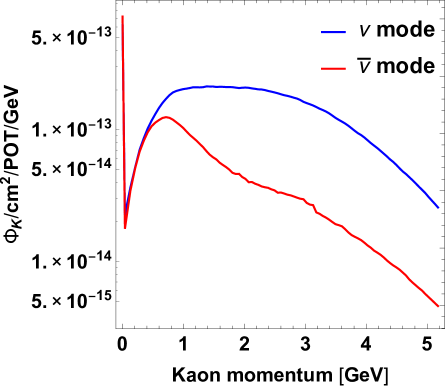
Figure 7: Kaon fluxes aiming at the MiniBooNE detector that were obtained from applying an inverse Lorentz boost on the muon (anti) neutrino. For details see text.

The heavy neutrino flux:

Next we will construct the heavy neutrino flux $\Phi_{N}(p_{N})$. We start with the assumption that the momenta of the heavy neutrinos are parallel to the parent kaons, i.e. $\vec{p}_{N}||\,\vec{p}_{K}$. This simplification allows us to construct the heavy neutrino flux $\Phi_{N}(p_{N})$ from the kaon flux $\Phi_{K}(p_{K})$ via Lorentz boosting the momentum $|\vec{p}_{N,0}|$ from the rest frame of the kaon with momentum $|\vec{p}_{K}|$

$$|\vec{p}_{N}|=\frac{|\vec{p}_{K}|}{m_{K}}E_{N,0}+\frac{E_{K}}{m_{K}}|\vec{p}_{N,0}|\cos\theta\,,$$ (28)

where the heavy neutrino momentum in the meson rest frame is given by

$$|\vec{p}_{N,0}|=\frac{\sqrt{(m_{K}^{2}-\Delta^{2})(m_{K}^{2}-\Sigma^{2})}}{2m_{K}}\,,\qquad\Delta=m_{N}-m_{\ell}\,,\qquad\Sigma=m_{N}+m_{\ell}\,.$$ (29)

For $m_{N}$ comparable to $m_{K}$ and for sufficiently large $|\vec{p}_{K}|$, also heavy neutrinos that are emitted backwards with respect to $\vec{p}_{K}$ can reach the detector. This means, from the kaon flux we construct two heavy neutrino fluxes: one from the forward emitted $N$ with $\cos\theta=+1$, and one from the backward emitted $N$ with $\cos\theta=-1$. Both, the backward $\Phi^{\rm bwd}_{N}(p_{N})$ and the forward $\Phi^{\rm fwd}_{N}(p_{N})$ emitted fluxes are normalized to the original light neutrino flux $\Phi_{\nu_{\mu}}(p_{\nu_{\mu}})$. The peak in the kaon spectrum from the stopped kaons (shown in figure 7) gives rise to monochromatic heavy neutrinos of energy $p_{N,0}$. We add this separately to the analysis and call it the “monochromatic peak”.

Geometrical acceptance:

We work under the assumption that the kaon momentum is always parallel to the beam line. In the experiment, neutrinos (light or heavy) are not produced with $\cos\theta=\pm 1$, but rather with an angle $\theta=0+\delta\theta,\pi-\delta\theta$, such that $|\cos\theta|=1-\varepsilon$. This deviation $\varepsilon$ stems from the angles that are smaller than or equal to the solid angle of the detector, which we approximate with $\theta_{D}\approx\tan\theta_{D}=r/L$, where $r$ is the radius of the detector and $L$ is the distance from the source. The maximal acceptance angle of the heavy neutrino in the lab frame is given by

$$\theta_{D}=\frac{|p_{N,\bot}|}{|p_{N,\parallel}|}=\frac{p_{N,0}\sin\theta^{\rm rest}_{N}}{\frac{p_{K}}{m_{K}}E_{N,0}+\frac{E_{K}}{m_{K}}p_{N,0}\cos\theta^{\rm rest}_{N}}\,,$$ (30)

here $\theta^{\rm rest}_{N}$ is the kaon rest frame decaying angle. The component of the momentum perpendicular to the beam line is not affected by the kaon boost and the parallel one is given by expression (28). For small angles $\sin\theta\sim\theta$, $\cos\theta\sim\pm 1$, the acceptance angle in the rest frame, for the backward and the forward decay, can be easily solved:

$$\theta^{\rm rest}_{N}=\frac{m_{K}}{p_{N,0}}\left(p_{K}E_{N,0}\pm E_{K}p_{N,0}\right)\theta_{D}\,.$$ (31)

Since the decay in the rest frame is isotropic, the heavy neutrino flux can be corrected by adding a geometrical factor given by the ratio between the maximum acceptance angles in the kaon rest frame for the heavy and light neutrinos:

$$f^{\rm fwd}=\frac{\theta^{\rm rest,\,fwd}_{N}}{\theta_{\nu}^{\rm rest}}\,;\quad f^{\rm bwd}=\frac{\theta^{\rm rest,\,bwd}_{N}}{\theta_{\nu}^{\rm rest}}\,.$$ (32)

Here we assume that the angular acceptance for light neutrinos is already included in $\Phi_{\nu_{\mu}}$ as provided by the collaboration. For small angles, eq. (32) turns into

$$f^{\rm fwd}(p_{K})=\frac{\left(p_{K}E_{N,0}+E_{K}p_{N,0}\right)}{p_{N,0}\left(p_{K}+E_{K}\right)}\,;\quad f^{\rm bwd}(p_{K})=\frac{\left(p_{K}E_{N,0}-E_{K}p_{N,0}\right)}{p_{N,0}\left(p_{K}+E_{K}\right)}\,.$$ (33)

Note that only the light neutrinos decaying in the forward direction reach the detector, so the heavy neutrino acceptance angle, for both backward and forward directions, have to be compared to the light neutrino one in the forward direction.

We have checked that for the kaon energies at MiniBooNE the small angle approximation (33) works very well. On the other hand for the kaon energies in NOMAD, this approximation does not hold because the kaon momentum can be larger. We have checked that taking the approximated expression for the geometrical factor for the NOMAD prediction gives an extra enhancement, i.e., we are somewhat over-predicting the number of events in NOMAD. This makes the limit somewhat too strong and is therefore conservative in what concerns the consistency with MiniBooNE, and hence we stick to the approximated expression.

The geometrical factors (33) can be expressed as a function of the heavy neutrino momentum performing an inverse boost

$$\frac{p_{K}}{m_{K}}E_{N}+\frac{E_{N}}{m_{K}}p_{N}=\pm p_{N,0}\,.$$

Solving for $p_{K}$ we obtained

$$p_{K}=\mp\frac{m_{K}}{m_{N}^{2}}E_{N}p_{N,0}+\frac{m_{K}}{m_{N}}\sqrt{\left(\frac{E_{N}\,p_{N,0}}{m_{N}}\right)^{2}+p_{N}^{2}-p_{N,0}^{2}}\,,$$

where upper (lower) signs apply to the forward (backward) geometrical factors. Note that in the forward decay case $p_{N}$ starts from $p_{N,0}$ and in the backward decay from 0.

Finally, the heavy neutrino flux is given by:

$$\Phi_{N}(p_{N})=f^{\rm fwd}(p_{N},m_{N})\Phi^{\rm fwd}_{N}(p_{N},m_{N})+f^{\rm bwd}(p_{N},m_{N})\Phi^{\rm bwd}_{N}(p_{N},m_{N})\,.$$

Appendix B Impact of the timing cut

The timing cut of 1.6$\mu$s after each beam spill discussed in sec. 3.1 has a strong impact on the predicted event spectrum, since it removes events from “slow” heavy neutrinos, which would provide a less forward peaked angular distribution for the photon events. In order to illustrate the importance of the timing cut, we show in this appendix results without requiring arrival within 1.6$\mu$s, i.e., we include all events from $N$ decays in the predicted signal.

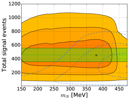
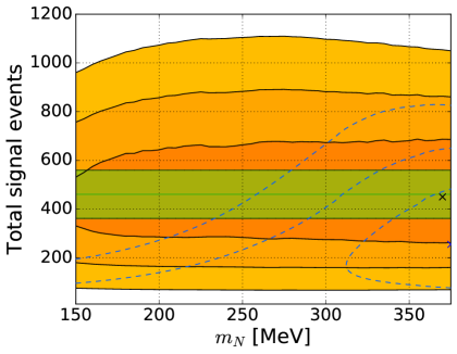
Figure 8: Allowed regions at 1, 2, and 3$\sigma$ for the energy (orange regions) and angular (dashed blue curves) in the $N_{\rm total}$ versus $m_{N}$ parameter space, without imposing the 1.6$\mu$s timing cut. The left (right) panel assumes heavy neutrino mixing with the electron (muon). The best fit of the energy spectral (angular) fit is indicated with a black (blue) cross. In green we show the measured excess of events and its 1$\sigma$ uncertainty.

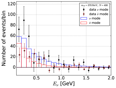
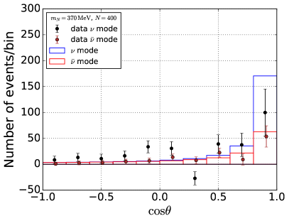
Figure 9: Predicted energy (left) and angular (right) spectra for $m_{N}=370\,{\rm MeV}$ and $N_{\rm total}=400$, without imposing the 1.6$\mu$s timing cut. The dots are the data with background subtracted, where each background component is re-scaled by the corresponding pull parameter obtained from the fit. Error bars include statistical and systematical errors.

From Fig. 8 we see that in this case also the angular fit shows preference for non-zero signal event numbers, and the $1\sigma$ allowed regions overlap between the energy and angular spectral fits. The best fit point for the energy spectrum degrades only marginally from $\chi^{2}_{\rm min}/{\rm dof}=58.1/36$ with timing cut to 62.8/36 without timing cut in the case of muon mixing. For the electron mixing we obtain an energy spectrum best fit with $\chi^{2}_{\rm min}/{\rm dof}=61.9/36$. Without the timing cut the angular fit yields $\chi^{2}_{\rm min}/{\rm dof}=32.1/18\,(30.0/18)$ for the mixing with the muon (electron), corresponding to a $p$-value of 1.1% (3.7%). In Fig. 9 we show the resulting energy and angular spectra for an example point in the $1\sigma$ overlap region. In comparison with fig. 4 we clearly observe an improved angular fit, while still maintaining a good description of the energy distribution. As discussed in the main text, the formally still rather low $p$-value is a consequence of the scattered data points with small error bars in the tail of the distributions.

References

- [1] MiniBooNE, A. A. Aguilar-Arevalo et al., Significant Excess of ElectronLike Events in the MiniBooNE Short-Baseline Neutrino Experiment, Phys. Rev. Lett. 121 (2018), no. 22 221801, [1805.12028].
- [2] MiniBooNE, A. A. Aguilar-Arevalo et al., Improved Search for Oscillations in the MiniBooNE Experiment, Phys. Rev. Lett. 110 (2013) 161801, [1303.2588].
- [3] LSND, A. Aguilar-Arevalo et al., Evidence for neutrino oscillations from the observation of anti-neutrino(electron) appearance in a anti-neutrino(muon) beam, Phys. Rev. D64 (2001) 112007, [hep-ex/0104049].
- [4] M. Dentler, A. Hernández-Cabezudo, J. Kopp, P. A. N. Machado, M. Maltoni, et al., Updated Global Analysis of Neutrino Oscillations in the Presence of eV-Scale Sterile Neutrinos, JHEP 08 (2018) 010, [1803.10661].
- [5] S. Gariazzo, C. Giunti, M. Laveder, and Y. F. Li, Updated Global 3+1 Analysis of Short-BaseLine Neutrino Oscillations, JHEP 06 (2017) 135, [1703.00860].
- [6] A. Diaz, C. A. Arguelles, G. H. Collin, J. M. Conrad, and M. H. Shaevitz, Where Are We With Light Sterile Neutrinos?, 1906.00045.
- [7] J. R. Jordan, Y. Kahn, G. Krnjaic, M. Moschella, and J. Spitz, Severe Constraints on New Physics Explanations of the MiniBooNE Excess, Phys. Rev. Lett. 122 (2019), no. 8 081801, [1810.07185].
- [8] P. Ballett, S. Pascoli, and M. Ross-Lonergan, MeV-scale sterile neutrino decays at the Fermilab Short-Baseline Neutrino program, JHEP 04 (2017) 102, [1610.08512].
- [9] S. N. Gninenko, The MiniBooNE anomaly and heavy neutrino decay, Phys. Rev. Lett. 103 (2009) 241802, [0902.3802].
- [10] S. N. Gninenko, A resolution of puzzles from the LSND, KARMEN, and MiniBooNE experiments, Phys. Rev. D83 (2011) 015015, [1009.5536].
- [11] E. Bertuzzo, S. Jana, P. A. N. Machado, and R. Zukanovich Funchal, Dark Neutrino Portal to Explain MiniBooNE excess, Phys. Rev. Lett. 121 (2018), no. 24 241801, [1807.09877].
- [12] P. Ballett, S. Pascoli, and M. Ross-Lonergan, U(1)’ mediated decays of heavy sterile neutrinos in MiniBooNE, Phys. Rev. D99 (2019) 071701, [1808.02915].
- [13] ISTRA+, V. A. Duk et al., Search for Heavy Neutrino in Decay at ISTRA+ Setup, Phys. Lett. B710 (2012) 307–317, [1110.1610].
- [14] M. Masip, P. Masjuan, and D. Meloni, Heavy neutrino decays at MiniBooNE, JHEP 01 (2013) 106, [1210.1519].
- [15] G. Magill, R. Plestid, M. Pospelov, and Y.-D. Tsai, Dipole Portal to Heavy Neutral Leptons, Phys. Rev. D98 (2018), no. 11 115015, [1803.03262].
- [16] E. Ma, G. Rajasekaran, and I. Stancu, Hierarchical four neutrino oscillations with a decay option, Phys. Rev. D61 (2000) 071302, [hep-ph/9908489].
- [17] S. Palomares-Ruiz, S. Pascoli, and T. Schwetz, Explaining LSND by a decaying sterile neutrino, JHEP 09 (2005) 048, [hep-ph/0505216].
- [18] C. Dib, J. C. Helo, M. Hirsch, S. Kovalenko, and I. Schmidt, Heavy Sterile Neutrinos in Tau Decays and the MiniBooNE Anomaly, Phys. Rev. D85 (2012) 011301, [1110.5400].
- [19] C. A. Arguelles, M. Hostert, and Y.-D. Tsai, Testing New Physics Explanations of MiniBooNE Anomaly at Neutrino Scattering Experiments, 1812.08768.
- [20] R. E. Shrock, General Theory of Weak Leptonic and Semileptonic Decays. 1. Leptonic Pseudoscalar Meson Decays, with Associated Tests For, and Bounds on, Neutrino Masses and Lepton Mixing, Phys. Rev. D24 (1981) 1232.
- [21] A. Aparici, K. Kim, A. Santamaria, and J. Wudka, Right-handed neutrino magnetic moments, Phys. Rev. D80 (2009) 013010, [0904.3244].
- [22] L. Duarte, J. Peressutti, and O. A. Sampayo, Majorana neutrino decay in an Effective Approach, Phys. Rev. D92 (2015), no. 9 093002, [1508.01588].
- [23] J. M. Butterworth, M. Chala, C. Englert, M. Spannowsky, and A. Titov, Higgs phenomenology as a probe of sterile neutrinos, 1909.04665.
- [24] P. Coloma, P. A. N. Machado, I. Martínez-Soler, and I. M. Shoemaker, Double-Cascade Events from New Physics in Icecube, Phys. Rev. Lett. 119 (2017), no. 20 201804, [1707.08573].
- [25] I. M. Shoemaker and J. Wyenberg, Direct Detection Experiments at the Neutrino Dipole Portal Frontier, Phys. Rev. D99 (2019), no. 7 075010, [1811.12435].
- [26] A. Atre, T. Han, S. Pascoli, and B. Zhang, The Search for Heavy Majorana Neutrinos, JHEP 05 (2009) 030, [0901.3589].
- [27] K. Bondarenko, A. Boyarsky, D. Gorbunov, and O. Ruchayskiy, Phenomenology of GeV-scale Heavy Neutral Leptons, JHEP 11 (2018) 032, [1805.08567].
- [28] A. D. Dolgov, S. H. Hansen, G. Raffelt, and D. V. Semikoz, Heavy Sterile Neutrinos: Bounds from Big Bang Nucleosynthesis and Sn1987A, Nucl. Phys. B590 (2000) 562–574, [hep-ph/0008138].
- [29] G. M. Fuller, A. Kusenko, and K. Petraki, Heavy Sterile Neutrinos and Supernova Explosions, Phys. Lett. B670 (2009) 281–284, [0806.4273].
- [30] T. Rembiasz, M. Obergaulinger, M. Masip, M. A. Perez-Garcia, M.-A. Aloy, et al., Heavy sterile neutrinos in stellar core-collapse, Phys. Rev. D98 (2018), no. 10 103010, [1806.03300].
- [31] MiniBooNE, A. A. Aguilar-Arevalo et al., The Neutrino Flux prediction at MiniBooNE, Phys. Rev. D79 (2009) 072002, [0806.1449].
- [32] MiniBooNE, A. A. Aguilar-Arevalo et al., The MiniBooNE Detector, Nucl. Instrum. Meth. A599 (2009) 28–46, [0806.4201].
- [33] W. Louis, private communication, 2019.
- [34] NA62, E. Cortina Gil et al., Search for heavy neutral lepton production in decays, Phys. Lett. B778 (2018) 137–145, [1712.00297].
- [35] E949, A. V. Artamonov et al., Search for heavy neutrinos in decays, Phys. Rev. D91 (2015), no. 5 052001, [1411.3963]. [Erratum: Phys. Rev.D91,no.5,059903(2015)].
- [36] NOMAD, C. T. Kullenberg et al., A search for single photon events in neutrino interactions, Phys. Lett. B706 (2012) 268–275, [1111.3713].
- [37] F. Vannucci, The NOMAD Experiment at CERN, Adv. High Energy Phys. 2014 (2014) 129694.
- [38] NOMAD, P. Astier et al., Prediction of neutrino fluxes in the NOMAD experiment, Nucl. Instrum. Meth. A515 (2003) 800–828, [hep-ex/0306022].
- [39] E. Goudzovski, 2019. talk at the International Conference on Kaon Physics 2019, Perugia, Italy, 10-13 Sept. 2019, https://indico.cern.ch/event/769729.
- [40] H. K. Dreiner, C. Hanhart, U. Langenfeld, and D. R. Phillips, Supernovae and Light Neutralinos: Sn1987A Bounds on Supersymmetry Revisited, Phys. Rev. D68 (2003) 055004, [hep-ph/0304289].
- [41] PS-191, F. Vannucci, Decays and oscillations of neutrinos in the ps-191 experiment, in Perspectives in electroweak interactions, leptonic session, 20th Rencontres de Moriond, Les Arcs, France, March 17-23, 1985. Vol. 2, pp. 277–285, 1985.
- [42] G. Bernardi et al., Further limits on heavy neutrino couplings, Phys. Lett. B203 (1988) 332–334.
- [43] G. Bernardi et al., Anomalous Electron Production Observed in the CERN Ps Neutrino Beam, Phys. Lett. B181 (1986) 173–177.
- [44] P. Astier et al., A Search for Neutrino Oscillations, Nucl. Phys. B335 (1990) 517–545.
- [45] KARMEN, B. Armbruster et al., Upper limits for neutrino oscillations muon-anti-neutrino electron-anti-neutrino from muon decay at rest, Phys. Rev. D65 (2002) 112001, [hep-ex/0203021].
- [46] T2K, K. Abe et al., Search for heavy neutrinos with the T2K near detector ND280, 1902.07598.
- [47] T2K, K. Abe et al., Search for neutral-current induced single photon production at the ND280 near detector in T2K, J. Phys. G46 (2019), no. 8 08LT01, [1902.03848].
- [48] MicroBooNE, LAr1-ND, ICARUS-WA104, M. Antonello et al., A Proposal for a Three Detector Short-Baseline Neutrino Oscillation Program in the Fermilab Booster Neutrino Beam, 1503.01520.
- [49] P. A. Machado, O. Palamara, and D. W. Schmitz, The Short-Baseline Neutrino Program at Fermilab, Ann. Rev. Nucl. Part. Sci. 69 (2019) [1903.04608].
- [50] L. Alvarez-Ruso and E. Saul-Sala, Radiative decay of heavy neutrinos at MiniBooNE and MicroBooNE, in Proceedings, Prospects in Neutrino Physics (NuPhys2016): London, UK, December 12-14, 2016, 2017. 1705.00353.