Magnetic circular dichroism in hard x-ray Raman scattering as a probe of local spin polarization

Abstract

We argue that the magnetic circular dichroism (MCD) of the hard x-ray Raman scattering (XRS) could be used as an element selective probe of local spin polarization. The magnitude of the XRS-MCD signal is directly proportional to the local spin polarization when the angle between the incident wavevector and the magnetization vector is $135^{\circ}$ or $-45^{\circ}$ . By comparing the experimental observation and the configuration interaction calculation at the $L_{2,3}$ and $M_{2,3}$ edges of ferromagnetic iron, we suggest that the integrated MCD signal in terms of the transferred energy could be used to estimate the local spin moment even in the case where the application of the spin sum-rule in X-ray absorption is questionable. We also point out that XRS-MCD signal could be observed at the $M_{1}$ edge with a magnitude comparable to that at the $M_{2,3}$ edge, although the spin-orbit coupling is absent in the core orbital. By combining the XRS-MCD at various edges, spin polarization distribution depending on the orbital magnetic quantum number would be determined.

I Introduction

X-ray magnetic circular dichroism (MCD) has been one of the powerful tools to investigate the electronic structure in magnetic materials. Particularly, owing to the orbital and spin sum-rules,(Carra et al., 1993; Thole et al., 1992) the MCD in the soft x-ray absorption spectroscopy (XAS) has been playing crucial roles for elucidating the electronic structure at and around the absorption site.(Nakamura and Suzuki, 2013) The MCD measurements in x-ray emission and resonant inelastic scattering are also important tools to clarify the electronic excitations in magnetic materials.(Kotani and Shin, 2001)

Recently, the MCD in the hard x-ray Raman scattering (XRS) at the Fe $\mathrm{L}_{2,3}$-edges in the ferromagnetic iron has been investigated.(Hiraoka et al., 2015; Takahashi and Hiraoka, 2015) The XRS is a kind of non-resonant inelastic x-ray scattering.(Rueff and Shukla, 2010) In the process of photon scattering, where an incident photon of energy $\hbar\omega_{\mathrm{i}}$ is absorbed and a photon of energy $\hbar\omega_{\mathrm{f}}$ is emitted, the electron system in the initial ground state of the energy $E_{\mathrm{i}}$ is excited to the final state of the energy $E_{\mathrm{f}}=E_{\mathrm{i}}+\hbar\omega_{\mathrm{i}}-\hbar\omega_{\mathrm{f}}$. The final state of the XRS is essentially the same with that of XAS: A core hole is left behind at the scattering site and an electron is added to the valence or conduction state. Therefore, the XRS intensity as a function of transferred energy is similar to the soft x-ray absorption coefficient as a function of the incident photon energy. Contrasting to the XAS, the hard-in-hard-out feature of the XRS is preferable for bulk sensitive measurements or the measurements under extreme conditions. In addition, the XRS can access the final states that are inaccessible by the dipole transition, because the non-dipole transition matrix elements become significant for shallow core excitation. By virtue of these features, the inner-core-exciting XRS has been demonstrating its usefulness particularly to unveil the electronic state of materials under extreme conditions.(Sternemann and Wilke, 2016) Recently, the electronic state of Fe in $\mathrm{Fe_{2}SiO_{4}}$, $\mathrm{Fe_{2}O_{3}}$ and $\mathrm{FeS}$ under high pressure is discussed by analyzing the XRS spectra at the Fe $M_{2,3}$ edge, and a spin transition is revealed from the change of spectral curves in $\mathrm{FeS}$.(Nyrow et al., 2014a, b) In addition, XRS at the rare earth $N$ and $O$ edges has been extensively discussed.(van der Laan, 2012; Huotari et al., 2015)

The XAS-MCD measurements are carried out in order to elucidate the orbital and spin magnetic moment at the selected magnetic ion. In the analysis of the MCD signal, the orbital- and the spin moment sum rules play central roles. However, it is also known that the spin sum rule has some limitations. The core hole level $j=l\pm 1/2$ should be clearly separated for safe application of the sum rule. Teramura et al. showed that the deviation of the rule could amount to 30% for $\mathrm{Mn}^{2+}$ and reached at 230% for Sm.(Teramura et al., 1996a, b) The XAS-MCD signal can be observed also at the $M_{2,3}$ edge of transition metals.(Yoshida and Jo, 1991; Koide et al., 1991) However, it is quite difficult to obtain the information about the local spin moment from the observed MCD signal alone, because it is quite hard to apply the spin sum rule due to the smallness of the spin orbit coupling (SOC) of the 3p hole, the strong 3p-3d Coulomb interaction, and the remarkable super-Coster-Kroning decay.(Coster and Kronig, 1935) The MCD signal at the $\mathrm{K}$-edge of transition metals also have been observed. While it is bulk sensitive, we can only indirectly obtain the information about orbital moment of the 3d state through the interaction between the 3d and 4p states.(Igarashi and Hirai, 1994, 1996; Brouder et al., 1996) It is worth noting that the spin sum rule(Thole and van der Laan, 1993; van der Laan and Thole, 1993) of the X-ray photoemission spectroscopy, in which both of the photon polarization and the spin of the emitted electron are exploited and the magnetic dichroism is observed in the emission of electrons, can be applied to estimate the ground state spin moment without the aforementioned shortcomings of the XAS-MCD spin sum rule.

The XRS-MCD signals have been observed at the $L_{2,3}$ edges of ferromagnetic iron by Hiraoka et al. (Hiraoka et al., 2015) The observe MCD spectral curves as a function of the transferred energy depend strongly on the angle $\alpha_{\mathrm{M}}$ (see fig. 1.), which is similar to the XAS-MCD spectral curve at the angle $\alpha_{\mathrm{M}}\sim 0^{\circ}$ . In the previous paper,(Takahashi and Hiraoka, 2015) we analyzed the XRS-MCD signals within a one-electron theory and discussed the relation between the spectral shape of the MCD signal and the angle $\alpha_{\mathrm{M}}$. We elucidated that the XRS-MCD signals can be considered as a result of the interference of the scattering amplitude due to the charge transition with that due to the electric, the orbital magnetic, and the spin magnetic transitions; their effects differently depend on the angle $\alpha_{\mathrm{M}}$. Particularly, at $\alpha_{\mathrm{M}}=135^{\circ}$ or $-45^{\circ}$, the magnitude of the XRS-MCD signal is proportional only to the local spin polarization. Therefore, the integrated XRS-MCD signal could be also used as a probe of local spin moment.

The magnetic Compton scattering (MCS) technique,(Cooper et al., 2004) which reveals the distribution of the spin magnetic moment in the momentum space, and the x-ray magnetic diffraction (XMD)(Blume, 1985) also owes to the MCD effect. The mechanism causing the MCD in MCS and XMD is different from that in XAS. The interaction between the magnetic field of radiation and the electron spin and/or orbital magnetic moments brings about the MCD effects in MCS and XMD. On the other hand, in the XAS, the spin-orbit coupling in the inner shell plays essential roles in provoking the MCD signal, since the electric field of the radiation does not directly couple to the orbital and spin magnetic moments. In the XRS, both mechanisms can induce the MCD signal with the magnitude comparable to each other. In contrast to the MCS, XRS-MCD may have advantageous features: the element selectivity and the selection rules in transition process. At $\alpha_{\mathrm{M}}=135^{\circ}$, the interference of scattering amplitude due to the charge- and spin-transitions alone produces the MCD signal. Therefore, it is expected that the XRS-MCD measurement could be used as a probe of local spin polarization at the scattering site even if the SOC is absent.

The interaction between the 3p electrons and the 3d electrons is so large that the M-edge excitation spectrum is expected to sensitively reflect the 3d state. Besides the XRS or XAS, the M-edge excitation of transition metal has been well measured using Electron Energy Loss Spectroscopy (EELS), or $K\beta$ x-ray emission spectroscopy (XES). Utilizing the surface sensitivity, the EELS is used to study the electronic structure in thin films.(Garvie and Buseck, 2004) The signal of the $K\beta$ XES is bulk sensitive, and the spin dependent spectrum caused by the 3p-3d exchange interaction is useful to elucidate the 3d state.(Taguchi et al., 1997) The dichroic effect of the Fe $K\alpha_{1}$ emission spectrum has also recently been observed.(Inami, 2017) In addition to these techniques, XRS-MCD may become a useful technique to understand the electronic structures under extreme conditions with exploiting its bulk sensitivity, element and orbital selectivity.

In the next section, we briefly describe the XRS-MCD formula. The model used to simulate the electronic state at the scattering site is described in Section III. In Section IV we discuss the $L_{2,3}$ and $M_{2,3}$ edge XRS spectra by comparing the calculations and the observations. The XRS spectra at the $M_{1}$ edge is also demonstrated. The last section is devoted to the concluding remarks. Demonstrations of the XRS-MCD spin sum rule are involved in the last section.

II Scattering intensity and MCD signal

We assume that the electronic state is excited from the initial state $\Phi_{\mathrm{i}}$ with energy $E_{\mathrm{i}}$ to the final state $\Phi_{\mathrm{f}}$ with energy $E_{\mathrm{f}}$ by absorbing an incident photon of polarization $\boldsymbol{e}_{\mathrm{i}}$, wave vector $\boldsymbol{q}_{\mathrm{i}}$, and energy $\hbar\omega_{\mathrm{i}}$and emitting a photon of polarization $\boldsymbol{e}_{\mathrm{f}}$, wave vector $\boldsymbol{q}_{\mathrm{f}}$, and energy of $\hbar\omega_{\mathrm{f}}$. In the final state, a core hole is left behind at the scattering site and an electron is added to the valence or conduction state. The scattering intensity may be proportional to the factor $\sum_{\Phi_{\text{f}}}\left|\bigl{\langle}\Phi_{\text{f}}|\sum_{i}\hat{f}(\boldsymbol{x}_{i})|\Phi_{\text{i}}\bigr{\rangle}\right|^{2}\delta_{E}$. Here, $\delta_{E}$ represents the energy conservation delta function $\delta\left(\Delta E+E_{\mathrm{i}}-E_{\mathrm{f}}\right)$ with $\Delta E=\hbar\omega_{\mathrm{i}}-\hbar\omega_{\mathrm{f}}$; the operator $\hat{f}$ is approximately given by the sum of the charge, electric, orbital magnetic, and spin magnetic transition operators $\hat{f}_{\mathrm{C}}$, $\hat{f}_{\mathrm{E}}$, $\hat{f}_{\mathrm{O}}$, and $\hat{f}_{\mathrm{S}}$, which are given in equations (1a-1d);(Takahashi and Hiraoka, 2015) $\boldsymbol{x}_{i}$ refers to the position $\boldsymbol{r}_{i}$ and spin $\boldsymbol{s}_{i}$ operators of the $i$th electron. The transition operators $\hat{f}_{\mathrm{C}}$, $\hat{f}_{\mathrm{E}}$, $\hat{f}_{\mathrm{O}}$, and $\hat{f}_{\mathrm{S}}$ are derived as the first- and second-order perturbation in terms of the interaction between electrons and electromagnetic field in the non-relativistic Hamiltonian.(Fröhlich and Studer, 1993) The perturbation terms of the higher order than $\left(\hbar\omega_{\mathrm{i}}/m_{\mathrm{e}}c^{2}\right)^{2}$ may be safely ignored, where $m_{\mathrm{e}}c^{2}$ is the electron rest energy. To handle the second-order perturbation terms, we assume that a core electron is excited to form an intermediate state $\Phi_{n}$ and the electron successively comes down to an energy level near the lowest unoccupied state to form a final electronic state $\Phi_{\mathrm{f}}$, and take the non-resonant limit, in which we ignore the energy difference between the intermediate electronic state energy $E_{n}$ and the initial electronic state energy $E_{\mathrm{i}}$ in the energy denominator assuming $E_{n}-E_{\mathrm{i}}\ll\hbar\omega_{\mathrm{i}},\ \hbar\omega_{\mathrm{f}}$. Then, we exploit the completeness of the intermediate electronic state $\Phi_{n}$, and neglect the terms of the order $1-\omega_{\mathrm{f}}/\omega_{\mathrm{i}}$. Thus, the transition operators may be obtained as

$$\hat{f}{}_{\mathrm{C}}\left(\boldsymbol{x}\right)=\boldsymbol{e}_{\text{f}}\cdot\boldsymbol{e}_{\text{i}}e^{i\boldsymbol{Q}\cdot\boldsymbol{r}},$$ (1a)

$$\hat{f}{}_{\mathrm{E}}\left(\boldsymbol{x}\right)=\frac{i\Delta E}{\alpha m_{\mathrm{e}}c^{2}}\boldsymbol{A}\cdot\boldsymbol{G}\left(\boldsymbol{Q},\boldsymbol{r}\right),$$ (1b)

$$\hat{f}{}_{\mathrm{O}}\left(\boldsymbol{x}\right)=-\frac{iE_{Q}}{2m_{\mathrm{e}}c^{2}}\boldsymbol{A}\cdot\hat{\boldsymbol{Q}}\times\boldsymbol{L}\left(\boldsymbol{Q},\boldsymbol{r}\right),$$ (1c)

$$\hat{f}{}_{\mathrm{S}}\left(\boldsymbol{x}\right)=-\frac{i\overline{E}}{2m_{\mathrm{e}}c^{2}}\boldsymbol{h}\cdot\boldsymbol{\sigma}e^{i\boldsymbol{Q}\cdot\boldsymbol{r}},$$ (1d)

where $\boldsymbol{\sigma}$, $\boldsymbol{Q}$, $\boldsymbol{A},$and $\boldsymbol{h}$ are defined as $\boldsymbol{\sigma}=2\boldsymbol{s}/\hbar$, $\boldsymbol{Q}=\boldsymbol{q}_{\mathrm{i}}-\boldsymbol{q}_{\mathrm{f}}$, $\boldsymbol{A}=\left(\boldsymbol{e}_{\text{f}}\cdot\hat{\boldsymbol{q}}_{\text{i}}\right)\boldsymbol{e}_{\text{i}}+\left(\boldsymbol{e}_{\text{i}}\cdot\hat{\boldsymbol{q}}_{\text{f}}\right)\boldsymbol{e}_{\text{f}}$, and $\boldsymbol{h}=\frac{\hbar\omega_{\text{f}}}{\overline{E}}\left(\boldsymbol{e}_{\text{i}}\cdot\hat{\boldsymbol{q}}_{\text{f}}\right)\left(\hat{\boldsymbol{q}}_{\text{f}}\times\boldsymbol{e}_{\text{f}}\right)-\frac{\hbar\omega_{\text{i}}}{\overline{E}}\left(\boldsymbol{e}_{\text{f}}\cdot\hat{\boldsymbol{q}}_{\text{i}}\right)\left(\hat{\boldsymbol{q}}_{\text{i}}\times\boldsymbol{e}_{\text{i}}\right)+\boldsymbol{e}_{\text{f}}\times\boldsymbol{e}_{\text{i}}-\left(\hat{\boldsymbol{q}}_{\text{f}}\times\boldsymbol{e}_{\text{f}}\right)\times\left(\hat{\boldsymbol{q}}_{\text{i}}\times\boldsymbol{e}_{\text{i}}\right)$; $\hat{\boldsymbol{q}}_{\mathrm{i(f)}}$ and $\hat{\boldsymbol{Q}}$ are the unit vectors $\boldsymbol{q}_{\mathrm{i(f)}}/q_{\mathrm{i(f)}}$ and $\boldsymbol{Q}/Q$, respectively. $E_{Q}$, and $\bar{E}$ are energies defined as $E_{Q}=\hbar cQ,$ and $\bar{E}=\hbar\left(\omega_{\mathrm{i}}+\omega_{\mathrm{f}}\right)/2$, respectively. $\alpha$ is the fine structure constant. The operators $\hat{f}_{\mathrm{E}}$ and $\hat{f}_{\mathrm{O}}$ are deduced from the terms including the linear momentum operator $\boldsymbol{p}=-i\hbar\nabla$ using the formula given by Trammel.(Trammell, 1953) Vectors $\boldsymbol{G}\left(\boldsymbol{Q},\boldsymbol{r}\right)$ and $\boldsymbol{L}\left(\boldsymbol{Q},\boldsymbol{r}\right)$ are defined as $\boldsymbol{G}\left(\boldsymbol{Q},\boldsymbol{r}\right)=\frac{\alpha^{2}}{r_{\text{e}}}\boldsymbol{r}g\left(\boldsymbol{Q}\cdot\boldsymbol{r}\right)$ and $\boldsymbol{L}\left(\boldsymbol{Q},\boldsymbol{r}\right)=\frac{1}{2}\frac{\boldsymbol{\ell}}{\hbar}f\left(\boldsymbol{\boldsymbol{Q}}\cdot\boldsymbol{r}\right)+f\left(\boldsymbol{\boldsymbol{Q}}\cdot\boldsymbol{r}\right)\frac{1}{2}\frac{\boldsymbol{\ell}}{\hbar}$ with $g\left(x\right)=\frac{1}{ix}\left(e^{ix}-1\right)$, $f\left(x\right)=-2i\frac{d}{dx}g\left(x\right)$, and $\boldsymbol{\ell}=-i\hbar\boldsymbol{r}\times\nabla$; $r_{\mathrm{e}}$ is the classical electron radius. We refer to the transition processes described by the operators $\hat{f}_{\mathrm{C}}$, $\hat{f}_{\mathrm{E}}$, $\hat{f}_{\mathrm{O}}$, and $\hat{f}_{\mathrm{S}}$ as C-, E-, O-, and S-transition, respectively.

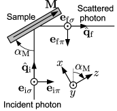
Figure 1: Schematics of scattering geometry in experiment. Coordinate and polarization vectors are defined as shown. $\alpha_{\mathrm{M}}$ is the angle between the magnetization vector $\boldsymbol{M}$ and the incident propagation vector $\boldsymbol{q}_{\mathrm{i}}$. The propagation vectors $\boldsymbol{q}_{\mathrm{i}}$ and $\boldsymbol{q}_{\mathrm{f}}$ of incident and emitted x-ray are perpendicular to each other.

The XRS-MCD experiment was carried out in the scattering geometry shown in figure 1. The wave vector $\boldsymbol{q}_{\mathrm{f}}$ is perpendicular to the incident wave vector $\boldsymbol{q}_{\mathrm{i}}$. In the experiment, the polarization of the emitted photon is not detected while the incident photon polarization is controlled. The polarization of the incident photon can be characterized by Stokes parameters $P_{1}$, $P_{2}$, and $P_{3}$.(Berestetskii et al., 1982) Since the magnitude of the C-transition matrix elements are much larger than the others, the total scattering intensity $I_{\mathrm{TOT}}=I\left(P_{1},P_{2},P_{3}\right)+I\left(P_{1},-P_{2},P_{3}\right)$ is approximately given only by the C-transition as $(1+P_{3})I_{\text{CC}}^{\sigma\sigma,\sigma\sigma}$ and the MCD signal $I_{\text{MCD}}=I\left(P_{1},\left|P_{2}\right|,P_{3}\right)-I\left(P_{1},-\left|P_{2}\right|,P_{3}\right)$ is given by $2\left|P_{2}\right|{\rm Im}(I_{\text{EC}}^{\sigma\pi,\sigma\sigma}+I_{\text{OC}}^{\sigma\pi,\sigma\sigma}+I_{\text{SC}}^{\sigma\pi,\sigma\sigma})$, where $\mathrm{Im}I$ represents the imaginary part of $I$; $I_{\text{EC}}^{\sigma\pi,\sigma\sigma}$ is given by

$$I_{\text{EC}}^{\sigma\pi,\sigma\sigma}(\Delta E)=I_{0}\sum_{\Phi_{\text{f}}}\sum_{i,i^{\prime}}\delta_{E}\bigl{\langle}\Phi_{\text{f}}|\hat{f}_{\text{E}}^{\sigma\pi}(\boldsymbol{x}_{i^{\prime}})|\Phi_{\text{i}}\bigr{\rangle}^{*}\bigl{\langle}\Phi_{\text{f}}|\hat{f}_{\text{C}}^{\sigma\sigma}\left(\boldsymbol{x}_{i}\right)|\Phi_{\text{i}}\bigr{\rangle},$$ (2)

with $I_{0}=r_{\mathrm{e}}^{2}\omega_{\mathrm{f}}/\omega_{\mathrm{i}}$. Here, the polarization vectors in the transition operator $\hat{f}_{\text{E}}^{\sigma\pi}$ are specified as $\boldsymbol{e}_{\mathrm{f}}=\boldsymbol{e}_{\mathrm{f}\sigma}$ and $\boldsymbol{e}_{\mathrm{i}}=\boldsymbol{e}_{\mathrm{i}\pi}$. $I_{\text{CC}}^{\sigma\sigma,\sigma\sigma}$, $I_{\text{OC}}^{\sigma\pi,\sigma\sigma}$ , and $I_{\text{SC}}^{\sigma\pi,\sigma\sigma}$ are also given in the same manner.

The XRS intensity may be described as the sum of the scattering intensity from each scattering site. We define the atomic transition matrix elements as
$F_{\mathrm{E}}^{\xi\eta}=\sum_{s_{z}}\int\psi_{\xi}^{*}\left(\boldsymbol{r},s_{z}\right)\hat{f}_{\mathrm{E}}^{\sigma\pi}(\boldsymbol{x})\psi_{\eta}\left(\boldsymbol{r},s_{z}\right)\mathrm{d}\boldsymbol{r}$, where indices $\xi$ and $\eta$ refer to one of the spin-orbitals in the 3d states and the 2p or 3p states at the scattering site, respectively; $s_{z}$ represents the spin magnetic quantum number. $F_{\mathrm{C}}^{\xi\eta}$, $F_{\mathrm{O}}^{\xi\eta}$, and $F_{\mathrm{S}}^{\xi\eta}$ are also defined in the same manner. In the following, the orbital and spin magnetic quantum number of the spin-orbital $\xi$($\eta$) are expressed as $m_{\xi(\eta)}$ and $z_{\xi(\eta)}$. Thus, the wave functions $\psi_{\xi}\left(\boldsymbol{r},s_{z}\right)$ might be given as a product of the radial wave-function $R_{\xi}\left(r\right)=R_{n_{\xi}l_{\xi}}\left(r\right)$, spherical harmonics $Y_{\xi}\left(\hat{\boldsymbol{r}}\right)=Y_{l_{\xi}m_{\xi}}\left(\hat{\boldsymbol{r}}\right)$, and spin function $\chi_{\xi}\left(s_{z}\right)=\chi_{z_{\xi}}\left(s_{z}\right)$,(Varshalovich et al., 1988) where $n_{\xi}=3$, $l_{\xi}=2$, $m_{\xi}=0,\pm 1,\pm 2$, and $z_{\xi}=\pm 1/2$. The wave function $\psi_{\eta}\left(\boldsymbol{r},s_{z}\right)$ is also written in the similar form. Functions $e^{i\boldsymbol{Q}\cdot\boldsymbol{r}}$, $g\left(\boldsymbol{Q}\cdot\boldsymbol{r}\right)$, and $f\left(\boldsymbol{Q}\cdot\boldsymbol{r}\right)$ can be written in the spherical harmonic expansion forms $4\pi\sum_{lm}Y_{lm}^{*}\left(\hat{\boldsymbol{Q}}\right)i^{l}w_{l}\left(Qr\right)Y_{lm}\left(\hat{\boldsymbol{r}}\right)$, where $w_{l}\left(x\right)$ is $j_{l}\left(x\right)$, $g_{l}\left(x\right)$, and $f_{l}\left(x\right)$; $j_{l}\left(x\right)$ is the spherical Bessel function with degree $l$, $g_{l}\left(x\right)=\frac{1}{x}\int_{0}^{x}j_{l}\left(t\right)dt$ and $f_{l}\left(x\right)=\frac{2}{x^{2}}\int_{0}^{x}tj_{l}\left(t\right)dt$, respectively.

For the scattering geometry as shown in figure 1, the atomic transition matrix elements are written as

$$F_{\mathrm{C}}^{\xi\eta}=4\pi\sum_{lm}i^{l}\tilde{j}_{l}\left(Q\right)Y_{lm}^{*}\left(\hat{\boldsymbol{Q}}\right)\left(Y_{lm}\right)_{\xi\eta},$$ (3a)

$$F_{\text{E}}^{\xi\eta}=\frac{4\pi i\Delta E}{\alpha m_{\text{e}}c^{2}}\sum_{lm\mu}i^{l}\tilde{g}_{l}\left(Q\right)Y_{lm}^{*}\left(\hat{\boldsymbol{Q}}\right)e_{\text{f}\sigma}^{\mu}\left(\hat{r}_{\mu}Y_{lm}\right)_{\xi\eta},$$ (3b)

$$F_{\text{O}}^{\xi\eta}=-\frac{4\pi iE_{Q}}{m_{\text{e}}c^{2}}\sum_{lm\mu}i^{l}\tilde{f}_{l}\left(Q\right)Y_{lm}^{*}\left(\hat{\boldsymbol{Q}}\right)\frac{v^{\mu}\left(\left[\ell_{\mu}Y_{lm}\right]\right)_{\xi\eta}}{4\hbar},$$ (3c)

$$F_{\text{S}}^{\xi\eta}=\frac{4\pi i\bar{E}}{m_{\text{e}}c^{2}}\sum_{lm\mu}i^{l}\tilde{j}_{l}\left(Q\right)Y_{lm}^{*}\left(\hat{\boldsymbol{Q}}\right)\hat{q}_{\text{f}}^{\mu}\left(\frac{\sigma_{\mu}}{2}Y_{lm}\right)_{\xi\eta},$$ (3d)

where $\left[\ell_{\mu}Y_{lm}\right]=\ell_{\mu}Y_{lm}+Y_{lm}\ell_{\mu}$ and the index $\mu$ runs over $1,0,-1$; $\tilde{j}_{l}\left(Q\right)$, $\tilde{g}_{l}\left(Q\right)$, and $\tilde{f}_{l}\left(Q\right)$ are radial integrals $\int R_{\xi}\left(r\right)h\left(r\right)R_{\eta}\left(r\right)r^{2}d\boldsymbol{r}$, where $h\left(r\right)$ is $j_{l}\left(Qr\right)$, $\frac{\alpha^{2}}{r_{\mathrm{e}}}rg_{l}\left(Qr\right)$, and $f_{l}\left(Qr\right)$, respectively. The bracket $\left(A\right)_{\xi\eta}$ represents the directional integral
$\sum_{s_{z}}\int Y_{\xi}^{*}\left(\hat{\boldsymbol{r}}\right)\chi_{\xi}\left(s_{z}\right)A\left(\hat{\boldsymbol{r}},\boldsymbol{s}\right)Y_{\eta}\left(\hat{\boldsymbol{r}}\right)\chi_{\eta}\left(s_{z}\right)d^{2}\hat{\boldsymbol{r}}$. The vector components $a^{\mu}$($a_{\mu}$) represent the spherical contravariant (covariant) components of vector $\boldsymbol{a}$.(Varshalovich et al., 1988) $\boldsymbol{v}$ is given by the vector product $\boldsymbol{e}_{\text{f}\sigma}\times\hat{\boldsymbol{Q}}$. The contravariant components $\left(a^{1},a^{0},a^{-1}\right)$ of the vectors $\boldsymbol{e}_{\mathrm{f}\sigma}$, $\hat{\boldsymbol{q}}_{\mathrm{f}}$, $\boldsymbol{v}$, and $\hat{\boldsymbol{Q}}$ can be written, as $(\frac{i}{\sqrt{2}},0,\frac{i}{\sqrt{2}}$), $(\frac{C_{\alpha}}{\sqrt{2}},S_{\alpha},\frac{-C_{\alpha}}{\sqrt{2}})$ , $(-\frac{C_{\beta}}{\sqrt{2}},-S_{\beta},\frac{C_{\beta}}{\sqrt{2}}$), and $(-\frac{S_{\beta}}{\sqrt{2}},C_{\beta},\frac{S_{\beta}}{\sqrt{2}})$, respectively, where $C_{\alpha}=\cos\alpha_{\mathrm{M}}$, $S_{\alpha}=\sin\alpha_{\mathrm{M}}$, $C_{\beta}=\cos(\alpha_{\mathrm{M}}+\gamma)$, and $S_{\beta}=\sin(\alpha_{\mathrm{M}}+\gamma)$ with $\gamma\approx\pi/4$.

The angle $\alpha_{\mathrm{M}}=135^{\circ}$ is found to be a special angle like as in XMD,(Blume and Gibbs, 1988; Lovesey, 1987; Laundy et al., 1991) which is called S-position. Because $\boldsymbol{Q}=\left(0,-1,0\right)$, thereby $Y_{lm}\left(\hat{\boldsymbol{Q}}\right)=\sqrt{\left(2l+1\right)/4\pi}\delta_{m0}$, the C-transition conserves both of the total orbital angular momentum $L_{z}$ and the total spin angular momentum $S_{z}$. The E- and O- transition change the orbital angular moment $L_{z}$ into $L_{z}\pm 1$ because the vector components $e_{\text{f}\sigma}^{0}$ and $v^{0}$ are zero so that only the matrix elements $\left(\hat{r}_{\pm 1}Y_{l0}\right)_{\xi\eta}$ and $\left(\left[\ell_{\pm 1}Y_{l0}\right]\right)_{\xi\eta}$ could be non-zero, while they conserve $S_{z}$. The S-transition conserves $L_{z}$, but changes $S_{z}$ into any of $S_{z}\pm 1$ and $S_{z}$. Inevitably, if we can assume that the electron system conserves the $z$ component of the total angular momentum $J_{z}=L_{z}+S_{z}$ around the scattering site when the electron system is not affected by the external perturbations, the interference terms $I_{\text{EC}}^{\sigma\pi,\sigma\sigma}$ and $I_{\text{OC}}^{\sigma\pi,\sigma\sigma}$ would be zero. The terms which involve the spin-off-diagonal S-transition in $I_{\mathrm{SC}}^{\sigma\pi,\sigma\sigma}$ also would be zero. Even in case the angular momentum $J_{z}$ is not conserved, if the powder approximation are allowed, the effect of such interference terms would not appear on the scattering intensity. Consequently, only the terms which involves the spin-diagonal S-transition in $I_{\text{SC}}^{\sigma\pi,\sigma\sigma}$ can contribute to the XRS intensity as MCD signal. Further, the term $I_{\text{S$\uparrow$C$\downarrow$}}^{\sigma\pi,\sigma\sigma}$ in $I_{\text{SC}}^{\sigma\pi,\sigma\sigma}$ consisting of the S$\uparrow$-transition, in which an up-spin electron is excited, and the C$\downarrow$-transition, in which a down electron is excited, and the term $I_{\text{S$\downarrow$C$\uparrow$}}^{\sigma\pi,\sigma\sigma}$ consisting of the S$\downarrow$-transition and the C$\uparrow$-transition would not contribute to the XRS intensity, because they have the same magnitude but have the opposite sign to each other. Therefore, putting $M_{m}=\sum_{\ell}M_{m}^{\left(\ell\right)}=\sum_{\ell}i^{\ell}\sqrt{4\pi\left(2l+1\right)}\tilde{j}_{\ell}\left(Q\right)\left(Y_{\ell 0}\right)_{2m,1m},$ the term $I_{\text{SC}}^{\sigma\pi,\sigma\sigma}\left(\Delta E\right)$ can be simplified as

$$I_{\text{SC}}^{\sigma\pi,\sigma\sigma}\left(\Delta E\right)=\frac{iI_{0}}{\sqrt{2}}\frac{\bar{E}}{m_{\text{e}}c^{2}}\sum_{\Phi_{\text{f}}}\delta\left(\Delta E+E_{\text{i}}-E_{\text{f}}\right)$$

$$\times\sum_{mm^{\prime}}M_{m^{\prime}}^{*}M_{m}\left\langle\Phi_{\text{i}}\left|p_{m^{\prime}\uparrow}^{\dagger}d_{m^{\prime}\uparrow}\right|\Phi_{\text{f}}\right\rangle\left\langle\Phi_{\text{f}}\left|d_{m\uparrow}^{\dagger}p_{m\uparrow}\right|\Phi_{\text{i}}\right\rangle$$

$$-\left\{\uparrow\longleftrightarrow\downarrow\right\}.$$ (4)

If we can assume that the 3p or 2p core states are completely occupied in the initial state $\Phi_{\mathrm{i}}$, the integrated $I_{\text{CC}}^{\sigma\sigma,\sigma\sigma}$ and $I_{\text{SC}}^{\sigma\pi,\sigma\sigma}$in terms of the transferred energy $\Delta E$ can be related to the hole number as

$$\int_{E_{\mathrm{E}}}^{E_{\mathrm{C}}}\mathrm{d}xI_{\text{CC}}^{\sigma\sigma,\sigma\sigma}\left(x\right)=I_{0}N_{1},$$ (5a)

$$\int_{E_{\mathrm{E}}}^{E_{\mathrm{C}}}\mathrm{d}x\mathrm{Im}I_{\text{SC}}^{\sigma\pi,\sigma\sigma}\left(x\right)=\frac{I_{0}}{2\sqrt{2}}\frac{\bar{E}}{m_{\text{e}}c^{2}}S_{1},$$ (5b)

where $E_{\mathrm{E}}$ and $E_{\mathrm{C}}$ indicate the transferred energy at the edge and an appropriate cutoff energy, respectively. $N_{1}$ and $S_{1}$ are defined as $N_{1}=\sum_{m=-1}^{1}\left|M_{m}\right|^{2}\left(h_{m\uparrow}+h_{m\downarrow}\right)$ and $S_{1}=\sum_{m=-1}^{1}\left|M_{m}\right|^{2}\left(h_{m\uparrow}-h_{m\downarrow}\right)$, and $h_{m\uparrow(\downarrow)}$ is the up (down) spin hole number in the 3d state specified by the orbital magnetic quantum number $m$. Thereby, we obtain

$$\frac{S_{1}}{N_{1}}=C\frac{\int_{E_{\mathrm{E}}}^{E_{\mathrm{C}}}\mathrm{d}xI_{\mathrm{MCD}}\left(x\right)}{\int_{E_{\mathrm{E}}}^{E_{\mathrm{C}}}\mathrm{d}xI_{\mathrm{TOT}}\left(x\right)},$$ (6)

with $C=\sqrt{2}\left(1+P_{3}\right)m_{\mathrm{e}}c^{2}/\left|P_{2}\right|\bar{E}$.

On the other hand, when the angle $\alpha_{\mathrm{M}}=0$ or $45\text{ degrees}$, which correspond to the L or L+S position in the XMD, the XRS-MCD signals may show complex behavior because both of $I_{\mathrm{EC}}$ and $I_{\mathrm{OC}}$ take part in the MCD signals. For the transition metal M-edge excitation, although the transferred energy $\Delta E$ is much smaller than that for the L-edge excitation, the E-transition is not negligible as shown later. If the transferred energy $\Delta E$ is so large that the contribution $I_{\mathrm{OC}}$ and $I_{\mathrm{SC}}$ is negligible, the sum-rules similar to those in the XAS-MCD might be established.

III Model Hamiltonian and Calculation Method

The configuration interaction (CI) calculation on the Anderson impurity model has been applied to analyze the signals from several core-level spectroscopic experiment on ferromagnetic nickel and have given consistent explanations to the different spectra based on the calculated electronic structure. (Jo and Sawatzky, 1991; Tanaka et al., 1992) Although the validity to apply this model for discussion on the spectroscopic properties of more strongly itinerant electron systems is not guaranteed, we exploit the CI calculation on this model as a makeshift to demonstrate the usefulness of the XRS-MCD in this study, because the electron-hole interaction is so large that independent particle approximation may not be suitable for describing the $\mathrm{M}_{2,3}$-edge excitation.

The 3d electron number of the Fe ion could be strongly fluctuating. We assume that the 3d electrons go back and forth between the 3d states under consideration and the electron reservoir states, which are supposed to have d-symmetric states consisting of the 3d and/or 4s states around the scattering site. We prepare the ten different levels $\nu_{\alpha m}$ ($\alpha=0,1$ and $m=-2,-1,\ldots,2$) as electron reservoir states. The initial electronic state might be symbolically expressed as $\left|\Phi_{\text{i}}\right\rangle=A\left|d^{8}\nu^{n_{0}+2}\right\rangle+B\left|d^{7}\nu^{n_{0}+3}\right\rangle+C\left|d^{6}\nu^{n_{0}+4}\right\rangle,$where $d^{m}\nu^{n}$ represents the configuration, in which $m$ electrons occupy the 3d states under consideration and $n$ electrons do the reservoir states. $A\left|d^{m}\nu^{n}\right\rangle$ represents the linear combination $\sum_{c}A_{c}\left|d^{m}\nu^{n}\right\rangle_{c}$ over the configurations belonging to the states specified as $d^{m}\nu^{n}$.

We assume the model Hamiltonian for simulating the electronic state as

$$H =\sum_{\xi}E_{d}n_{d\xi}+\sum_{\alpha\xi}E_{\alpha}n_{\alpha\xi}+\sum_{\alpha\xi}V\left(d_{\xi}^{\dagger}c_{\alpha\xi}+c_{\alpha\xi}^{\dagger}d_{\xi}\right)$$

$$+U_{dd}\sum_{\xi<\xi^{\prime}}n_{d\xi}n_{d\xi^{\prime}}+U_{pd}\sum_{\xi\eta}n_{d\xi}n_{p\eta}$$

$$+H_{dd}\left(F_{dd}^{2},F_{dd}^{4}\right)+H_{pd}\left(F_{pd}^{2},G_{pd}^{1},G_{pd}^{3}\right)$$

$$-\Delta_{\text{mol}}z_{\xi}n_{d\xi}+H_{d\text{SO}}\left(\zeta_{d}\right)+H_{p\text{SO}}\left(\zeta_{p}\right),$$ (7)

where, $d_{\xi}^{\dagger}$, $d_{\xi}$, and $n_{d\xi}$ represent the creation, annihilation, and number operators for the spin-orbital $\xi$ in the 3d state at the site under consideration. $c_{\alpha\xi}^{\dagger}$, $c_{\alpha\xi}$, and $n_{\alpha\xi}$ represent the creation, annihilation, and number operators for the spin orbital $\nu_{\alpha m_{\xi}z_{\xi}}$ in the reservoir states. $n_{p\eta}$ represents the number operator for the spin-orbital $\eta$ in the 2p or 3p states. The parameters $E_{d}$ and $E_{\alpha}$ representing the one electron level are assumed to be $0$ eV, $-0.2\times\alpha$ eV. The parameters $U_{dd}$ and $U_{pd}$ corresponding the averaged 3d-3d and 2p(3p)-3d Coulomb interaction are assumed to be $3.5$eV and $5.0$ ($3.5$) eV. The hybridization $V$ is assumed to be $1.1$ eV. The Slater integrals $F_{dd}^{2}$, $F_{dd}^{4}$, $F_{pd}^{2}$, $G_{pd}^{1}$, and $G_{pd}^{3}$ are assumed to be 80% of the atomic values. The parameters $\zeta_{d}$ and $\zeta_{p}$ of the spin-orbit coupling $H_{d\mathrm{SO}}$and $H_{p\mathrm{SO}}$ are assumed to be the atomic values. These atomic values are calculated by using Cowan code.(Cowan, 1981) We add the molecular field term $-\Delta_{\text{mol}}z_{\xi}n_{d\xi}$ in order to simulate the ferromagnetic ground state. The parameter $\Delta_{\mathrm{mol}}$ is assumed to be $1.9$eV, which corresponds to the observed exchange splitting value $\varepsilon\left(\mathrm{H}_{25\uparrow}\right)-\varepsilon\left(\mathrm{H}_{25\downarrow}\right)$.(Santoni and Himpsel, 1991) We numerically diagonalize the Hamiltonian to obtain the initial ground state, in which the d electron number, spin moment, and orbital moment are about $7.0$, $2.2\mu_{\mathrm{B}}$, and $0.054\mathrm{\mu_{B}}$, respectively. The weights $A$, $B$, and $C$ are $\left|A\right|^{2}=23.7\%$, $\left|B\right|^{2}=55.7\%$, and $\left|C\right|^{2}=20.6\%$, which may be consistent with the stronger itinerancy than ferromagnetic Ni.(Jo and Sawatzky, 1991; Tanaka et al., 1992)

Scattering operators $\hat{f}_{\mathrm{E}}^{\sigma\pi}$ can be expressed in the second quantization form using the atomic transition matrix elements $F_{\mathrm{E}}^{\xi\eta}$: $\hat{f}_{\mathrm{E}}^{\sigma\pi}=\sum_{\xi\eta}F_{\mathrm{E}}^{\xi\eta}d_{\xi}^{\dagger}p_{\eta}$ within the model used. The terms $I_{\mathrm{EC}}^{\sigma\pi,\sigma\sigma}$ are given by $I_{\text{EC}}^{\sigma\pi,\sigma\sigma}=\frac{I_{0}}{2\pi i}\left\langle\Phi_{\text{i}}\left|\hat{f}_{\text{E}}^{\dagger}\left[R\left(z\right)-R\left(z^{*}\right)\right]\hat{f}_{\text{C}}\right|\Phi_{\text{i}}\right\rangle,$where $R\left(z\right)=1/\left(z-H\right)$ with $z=\Delta E+E_{\text{i}}-H-i\Gamma$ and $z^{*}=\Delta E+E_{\text{i}}-H+i\Gamma$. The other terms $I_{\mathrm{CC}}^{\sigma\sigma,\sigma\sigma}$, $I_{\mathrm{OC}}^{\sigma\pi,\sigma\sigma}$, and $I_{\mathrm{SC}}^{\sigma\pi,\sigma\sigma}$ also can be given in the same manner. To calculate these terms we can use the recursion method with assuming that the final states be described as $\left|\Phi_{\text{f}}\right\rangle=A^{\prime}\left|p^{5}d^{9}\nu^{n_{0}+2}\right\rangle+B^{\prime}\left|p^{5}d^{8}\nu^{n_{0}+3}\right\rangle+C^{\prime}\left|p^{5}d^{7}\nu^{n_{0}+4}\right\rangle$, where $p^{n}$ indicates the states that $n$ electrons are accommodated in the 2p or 3p state. It is well known that the term-dependent core-hole lifetime due to the 3p-3d3d super-Coster-Kroning decay plays significant roles for explaining the observed spectral shape in the M-edge spectroscopy.(Okada et al., 1993) Such core-hole decay processes are not taken into account in our model Hamiltonian. Taguchi et al. assumed that the core-hole lifetime broadening $\Gamma$ of 3p hole is linear on the relative excitation energy in order to investigate the emission spectra from manganese oxides.(Taguchi et al., 1997) Although we have no substantial reasons, we assume the broadening $\Gamma$ linearly depending on the relative excitation energy, when comparing the calculated and observed spectra at the $M_{2,3}$ edge.

As shown later, we obtain plausible results for both of the $L_{2,3}$ and $M_{2,3}$ edges XRS spectra. The spectral shape is not sensitive on the model parameters as far as we use the initial state in which the 3d electron number is about $7.0$ and the spin moment is about $2.2\mathrm{\mu_{B}}$. However, the validity of the calculated spectra based on the above mentioned approximation is probably quite limited. In the spectral shape at the $M_{2,3}$ edge, several inconsistencies are found between the observation and the calculation. Nevertheless, we hope that the results are of value to provide insight into the XRS-MCD and understand its usefulness.

IV Results and Discussions

IV.1 Fe $L_{2,3}$ edge

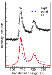
Figure 2: (color on line) Total XRS intensity as a function of the transferred energy and the calculated intensity $I_{\mathrm{CC}}$. Thin sold line with circle symbol represents the observed intensity without background subtraction. Thick solid, and broken lines are the spectral curves calculated by the CI calculation and the band structure calculation, respectively. Lifetime broadening is assumed to be $\Gamma_{3}=1.4$ and $\Gamma_{2}=0.9$ eV.

In the previous papers,(Hiraoka et al., 2015; Takahashi and Hiraoka, 2015) we investigated the XRS-MCD at the Fe $L_{2,3}$ edge within independent particle approximation using band structure calculation based on the local spin density approximation. At the $L_{2,3}$ edge, the dipole transitions dominates the scattering intensity and the MCD signal, in which the form factors $\tilde{j}_{1}\left(Q\right)$, $\tilde{g}_{0}\left(Q\right)$, and $\tilde{f}_{1}\left(Q\right)$ are relevant. In figure 2, we compare the total intensities calculated by the CI calculation and the band calculation with the experimental observation. Both of the calculations well reproduce the observed spectral curve. The observed $\mathrm{L}_{3}$ peak, concentrating around the transferred energy $705\sim 714\mathrm{eV}$, looks consisting of a main peak about $708\mathrm{eV}$ and a shoulder structure around $712\mathrm{eV}$. This shoulder structure seems not to be properly reproduced by the calculations: The one-body calculation does not give the shoulder structure, on the other hand the CI calculation seems to provide too strong intensity for the shoulder structure.

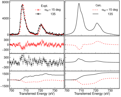
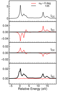
Figure 3: (color online) The observed total intensity after background subtraction (left) and the calculated total intensity (center) are shown in the top panels, respectively. The total XRS signals at $\alpha_{\mathrm{M}}=15^{\circ}$ and $135^{\circ}$ are shown with red dashed and black solid curves. MCD signals at the corresponding angle $\alpha_{\mathrm{M}}$ are shown in the second and third rows. The integrated MCD signals are shown in bottom panels. In the right panels, the spectral curves of the intensity $I_{\mathrm{CC}}$, $\mathrm{Im}I_{\mathrm{EC}}$, $\mathrm{Im}I_{\mathrm{OC}}$, and $\mathrm{Im}I_{\mathrm{SC}}$ at the angles $\alpha_{\mathrm{M}}=0^{\circ}$ and $135^{\circ}$ are shown with lifetime broadening $\Gamma=0.14\mathrm{eV}$.

The total intensity after background subtraction and the MCD signals are shown in figure 3 in comparison with those obtained by the CI calculation. The Stokes parameters of the incident beam polarization are assumed as $\left|P_{2}\right|=0.6$ and $P_{3}=-0.8$. The CI calculation well reproduces the observed MCD signals both on the relative intensity to the total intensity, the sign of MCD signal, and their dependence on the angle $\alpha_{\mathrm{M}}$. In the most right panels, the spectral curves of the intensity $I_{\mathrm{CC}}$, and the MCD components $\mathrm{Im}I_{\mathrm{EC}}$, $\mathrm{Im}I_{\mathrm{OC}}$, and $\mathrm{Im}I_{\mathrm{SC}}$ at the angle $\alpha_{\mathrm{M}}=0^{\circ}$ and $135^{\circ}$ are also shown. At the angle $\alpha_{\mathrm{M}}=0^{\circ}$ , $\mathrm{Im}I_{\mathrm{EC}}$ dominantly contributes to the total MCD signal, while at the angle $\alpha_{\mathrm{M}}=135^{\circ}$ , $\mathrm{Im}I_{\mathrm{EC}}$ and $\mathrm{Im}I_{\mathrm{OC}}$ are completely suppressed and only $\mathrm{Im}I_{\mathrm{SC}}$ contributes to the total MCD signal. We note that at the angle $\alpha_{\mathrm{M}}=0^{\circ}$, the MCD component $\mathrm{Im}I_{\mathrm{SC}}$ is not completely zero; it would be zero if we assume the powder approximation. The results obtained by the CI calculation are essentially the same with those calculated by the band calculation(Takahashi and Hiraoka, 2015).

IV.2 Fe $M_{2,3}$ edge

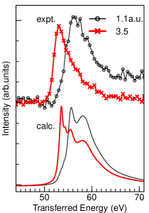
Figure 4: (Color online) Observed and calculated total XRS intensities as a function of the transferred energy. Black thin and red thick lines are the intensities at the scattering vector $Q=1.1$ and 3.5 a.u. corresponding to the scattering angles $2\theta=23^{\circ}$ and $90^{\circ}$, respectively.

The relative magnitude of $\mathrm{Im}I_{\mathrm{SC}}$ to $I_{\mathrm{CC}}$ is independent of the edges, because $I_{\mathrm{SC}}$ is directly proportional to the 3d spin moment in accordance with eq. (4). At the Fe $M_{2,3}$ edge, the MCD signal at the angle $\alpha_{\mathrm{M}}=135^{\circ}$ might be observed with the same relative magnitude to the total intensity as at the $L_{2,3}$ edge. At the Fe $M_{2,3}$ edge the octupole transition becomes significant as well as the dipole transition for the high $Q$ scattering. Figure 4 shows the observed and calculated total intensities as a function of the transferred energy at the scattering angles $2\theta=23^{\circ}$ and $90^{\circ}$ , which correspond to the scattering vector $Q=1.1$ and $3.5$ a.u., respectively. At the scattering angle $2\theta=23^{\circ}$ , the intensity is dominated by the dipole transition. As the scattering vector becomes larger, the octupole transition become dominant and the dipole transition becomes subordinate; the intensity around the transferred energy $53\sim 55$ eV become intense and the intensity above $55$ eV becomes weak. A similar tendency can be seen in the XRS spectra on iron oxides.(Nyrow et al., 2014b) In order to compare the observation and the calculation, we naively assume that the life-time broadening is $\Gamma=\max\left(0.1E+0.14,\,0.14\right)$ eV, where $E$ is the relative transferred energy from the edge. Although the calculated spectra resemble the observed one, they show discernible inconsistencies at the scattering angle $2\theta=90^{\circ}$. In comparison with the observed spectra, the calculated intensity above the transferred energy $55$ eV, which is mainly caused by the dipole transition, looks to be quite overestimated, or the intensity around the transferred energy $53$ eV, which is mainly caused by the octupole transition, looks to be underestimated. In order to improve the calculated spectral curve, it might be necessary to explicitly take account of the super-Coster-Kroning decay process into the calculation. In the vicinity of the edge, the low-lying electron-hole-pair excitations might be essential for the shape of the peak.(Doniach et al., 1971; Nozières and Abrahams, 1974) In spite of the noticeable deviation between the experimental observation and the calculation, we expect that the results could give us better understanding of the XRS-MCD.

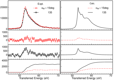
Figure 5: (color online) Observed spectra (left panel) and calculated spectra (right panel) are shown as a function of the transferred energy. The total intensity after subtracting the background, the MCD signal, and the integrated MCD signal are shown in top, middle, and bottom panels. The signals for the angle $\alpha_{\mathrm{M}}=15^{\circ}$ and $135^{\circ}$ are indicated by red cross symbols and broken lines, and the black circle symbols and solid lines.

Left panel in figure 5 shows the observed spectra as a function of the transferred energy at the angles $\alpha_{\mathrm{M}}=15^{\circ}$ and $135^{\circ}$. Contrasting to the L-edge spectra, the spectral curve of the MCD signal at $\alpha_{\mathrm{M}}=15^{\circ}$ is rather simple: its magnitude is very weak and the shape is similar to that at $\alpha_{\mathrm{M}}=135^{\circ}$, which are also similar to the total intensity. This might suggest that the contribution of $\mathrm{Im}I_{\mathrm{EC}}$ and $\mathrm{Im}I_{\mathrm{OC}}$ are suppressed and $\mathrm{Im}I_{\mathrm{SC}}$ dominates the MCD signal. Right panel shows the calculated spectra corresponding to the observation with the polarization parameters $\left|P_{2}\right|=0.6$ and $P_{3}=-0.8$. The sign of the MCD signal, the relative magnitude of the MCD signal to the total intensity and the shape of the spectral curves are rather well reproduced by the calculation.

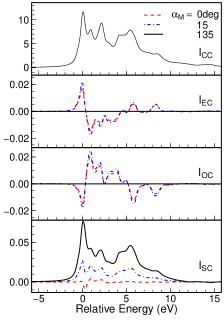
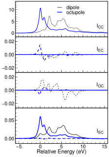
Figure 6: (Color online) Left panels show the intensities $I_{\mathrm{CC}}$, $\mathrm{Im}I_{\mathrm{EC}}$, $\mathrm{Im}I_{\mathrm{OC}}$, and $\mathrm{Im}I_{\mathrm{SC}}$ from top to bottom as a function of relative energy of the final states at $\alpha_{\mathrm{M}}=0$ (dashed line), $15^{\circ}$ (dot-dash line) and $135^{\circ}$ (solid line). Right panels show the decomposed intensities into the parts due to the dipole (thin line) and octupole (thick line) transition processes. Dashed and solid curves indicate the results at the angle $\alpha_{\mathrm{M}}=0^{\circ}$ and $135^{\circ}$. The life time broadening is assumed to be $\Gamma=0.14$ eV.

The left panel in figure 6 shows the intensities $I_{\mathrm{CC}}$ $\mathrm{Im}I_{\mathrm{EC}}$, $\mathrm{Im}I_{\mathrm{OC}}$, and $\mathrm{Im}I_{\mathrm{SC}}$ as a function of the relative energy of the final states at the angle $\alpha_{\mathrm{M}}=0^{\circ}$, $15^{\circ}$, and $135^{\circ}$. It is found that $\mathrm{Im}I_{\mathrm{EC}}$ and $\mathrm{Im}I_{\mathrm{OC}}$ can be almost canceled out to each other near $\alpha_{\mathrm{M}}=0^{\circ}$. Consequently, the the MCD signal at $\alpha_{\mathrm{M}}=15^{\circ}$ are dominated by $\mathrm{Im}I_{\mathrm{SC}}$. At the L-edge, this cancellation is insufficient: $\mathrm{Im}I_{\mathrm{EC}}$ dominates the MCD signals at $\alpha_{\mathrm{M}}=15^{\circ}$. At $\alpha_{\mathrm{M}}=135^{\circ}$, the MCD signals due to $\mathrm{Im}I_{\mathrm{EC}}$ and $\mathrm{Im}I_{\mathrm{OC}}$ are completely suppressed, so $\mathrm{Im}I_{\mathrm{SC}}$ alone contributes to the MCD signals. Thus, the MCD signals reflect only the spin polarization in the 3d orbitals of the orbital magnetic quantum number $m=0,\pm 1$. It may be worth noting again that $\mathrm{Im}I_{\mathrm{SC}}$ is not identically zero even at the angle $\alpha_{\mathrm{M}}=0^{\circ}$ .

The left panel in figure 6 shows the calculated intensities due to the dipole transition alone and the octupole transition alone. The dipole and octupole transitions dominate the intensities in the range of $2.5\sim 10$ eV and the range of $0\sim 2.5$ eV, respectively. The effect of the interference between them does not look significant in the intensity $I_{\mathrm{CC}}$. On the other hand it could not be ignored for producing the spectral structure of the MCD signal. Therefore, the detailed information about the electronic structure might be obtained from the analysis of the XRS-MCD signal.

IV.3 $M_{1}$ edge

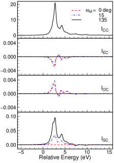
Figure 7: (Color online) The intensity $I_{\mathrm{CC}}$ and the MCD components $\mathrm{Im}I_{\mathrm{EC}}$, $\mathrm{Im}I_{\mathrm{OC}}$, and $\mathrm{Im}I_{\mathrm{SC}}$ as a function of relative energy of the final states at $\alpha_{\mathrm{M}}=0^{\circ}$ (dashed line), $15^{\circ}$ (dot-dash line) and $135^{\circ}$ (solid line) for the $M_{1}$ edge XRS. The life time broadening is assumed to be $\Gamma=0.14$ eV.

The MCD signal would be observed even at the $M_{1}$ edge with the magnitude comparable to the $M_{\mathrm{2,3}}$ edge, because $I_{\mathrm{SC}}$ reflects the 3d spin polarization through the interaction $\boldsymbol{h}\cdot\boldsymbol{\sigma}$ between the electron spin and the radiation field in Eq. (1d). The quadrupole transition, in which the factors $\tilde{j}_{2}\left(Q\right)$, $\tilde{g}_{1}\left(Q\right)$, and $\tilde{f}_{2}\left(Q\right)$ are relevant, dominates the excitation process (3s$\rightarrow$3d) at the $M_{1}$ edge. Due to the absence of the SOC in the 3s orbital, $\mathrm{Im}I_{\mathrm{EC}}$ and $\mathrm{Im}I_{\mathrm{OC}}$ are supposed to be small; those signals just reflect the 3d orbital polarization due to the SOC in the 3d states. It is expected that $\mathrm{Im}I_{\mathrm{SC}}$ would be as large as that in the $M_{2,3}$ edge. Thus, the MCD signal caused by only the 3d spin polarization would be observed.

In figure 7, the calculated $M_{1}$ edge XRS and the MCD spectra are shown. The relative magnitude of the MCD signal to the total intensity is in the same order with that in the $M_{2,3}$ edge spectra at the angle $\alpha_{\mathrm{M}}=135^{\circ}$. At this angle $\alpha_{\mathrm{M}}$, the MCD components $\mathrm{Im}I_{\mathrm{EC}}$ and $\mathrm{Im}I_{\mathrm{OC}}$ are suppressed, so that the component $\mathrm{Im}I_{\mathrm{SC}}$ alone contributes to the MCD signal. Therefore, the MCD signal reflects only the spin moment of the 3d orbital with the orbital magnetic quantum number $m=0$. At the angle $\alpha_{\mathrm{M}}=0^{\circ}$, the component $\mathrm{Im}I_{\mathrm{SC}}$ is almost suppressed because the SOC in 3s orbital is absent and the SOC in the 3d orbital is very small. The components $\mathrm{Im}I_{\mathrm{EC}}$ and $\mathrm{Im}I_{\mathrm{OC}}$ only weakly contribute to the MCD signal due to the smallness of the SOC in 3d orbital. Because they are very small and have opposite sign to each other, the total MCD signal would be too small to be observed at the present stage.

Putting $M_{0}^{\prime}=-\sqrt{12\pi}\tilde{j}_{2}\left(Q\right)\left(Y_{20}\right)_{20,00},$ the integrated intensity $I_{\text{CC}}^{\sigma\sigma,\sigma\sigma}$ and component $\mathrm{Im}I_{\text{SC}}^{\sigma\pi,\sigma\sigma}$ at the angle $\alpha_{\mathrm{M}}=135^{\circ}$ might be given by

$\int_{E_{\mathrm{E}}}^{E_{\mathrm{C}}}\mathrm{d}xI_{\text{CC}}^{\sigma\sigma,\sigma\sigma}\left(x\right)=I_{0}M_{0}^{\prime 2}\left(h_{0\uparrow}+h_{0\downarrow}\right)$, and $\int_{E_{\mathrm{E}}}^{E_{\mathrm{C}}}\mathrm{d}x\mathrm{Im}I_{\text{SC}}^{\sigma\pi,\sigma\sigma}\left(x\right)=\frac{1}{2\sqrt{2}}\frac{\bar{E}}{m_{\text{e}}c^{2}}I_{0}M_{0}^{\prime 2}\left(h_{0\uparrow}-h_{0\downarrow}\right)$, respectively. Therefore, the ratio of the integrated MCD signals to the integrated intensity could give the spin polarization ratio $\left(h_{0\uparrow}-h_{0\downarrow}\right)/\left(h_{0\uparrow}+h_{0\downarrow}\right)$ in the 3d orbitals with the magnetic quantum number $m=0$ as $C\int_{E_{\mathrm{E}}}^{E_{\mathrm{C}}}\mathrm{d}xI_{\mathrm{MCD}}\left(x\right)/\int_{E_{\mathrm{E}}}^{E_{\mathrm{C}}}\mathrm{d}xI_{\mathrm{TOT}}\left(x\right)$ with $C=\sqrt{2}\left(1+P_{3}\right)m_{\mathrm{e}}c^{2}/\left|P_{2}\right|\bar{E}$.

V Concluding remarks

We investigated the XRS-MCD spectra by comparing the observed and the theoretically calculated spectra at the $L_{2,3}$ and $M_{2,3}$ edges of ferromagnetic iron. We used the configuration interaction calculation on the Anderson impurity model as a makeshift to simulate the electronic structure of iron at the scattering center. The calculation reproduced the observed spectra rather well in spite of the awkward approximation for the strongly itinerant system. For more detailed analysis, we would need a more sophisticated approximation and a model which could appropriately reproduce the multiplet structure in the excited state with taking into account both of the localized and itinerant nature of the 3d electrons in the ferromagnetic iron. For the localized electronic systems, the model used here may give more plausible results.

The MCD signals consist of the three components $\mathrm{Im}I_{\mathrm{EC}}$, $\mathrm{Im}I_{\mathrm{OC}}$, and $\mathrm{Im}I_{\mathrm{SC}}$. Their angle $\alpha_{\mathrm{M}}$ dependences of them are different. Particularly, at $\alpha_{\mathrm{M}}=135^{\circ}$ in the right angle scattering condition, $\mathrm{Im}I_{\mathrm{EC}}$ and $\mathrm{Im}I_{\mathrm{OC}}$ are suppressed if the total $J_{z}$ around the scattering site is conserved or in the situation where the powder approximation is proper. At this scattering geometry, the orbital magnetic quantum number $m$ is conserved both in the C- and S- transitions. The intensity $I_{\mathrm{CC}}$ is proportional to the 3d hole number, while the MCD component $\mathrm{Im}I_{\mathrm{SC}}$ is proportional to the difference of the number of the up and down 3d holes. Therefore, the information of the spin polarization in the 3d orbitals with the magnetic quantum numbers $m=0,\pm 1$ may be obtained.

Here, we demonstrate the XRS-MCD spin sum rule at $\alpha_{\mathrm{M}}=135^{\circ}$. The ratios of the integrated MCD signal and the total signal in the observation $\int_{E_{\mathrm{E}}}^{E_{\mathrm{C}}}I_{\mathrm{MCD}}\left(x\right)\mathrm{d}x/\int_{E_{\mathrm{E}}}^{E_{\mathrm{C}}}I_{\mathrm{TOT}}\left(x\right)\mathrm{d}x$ is estimated to be $0.025\sim 0.031$ at the $L_{2,3}$ edge with $E_{\mathrm{E}}=700\sim 705$ and $E_{\mathrm{C}}=730\sim 740$ eV. The ratio at the $M_{2,3}$ edge is estimated to be $0.024\sim 0.029$ with $E_{\mathrm{E}}=45\sim 51$ and $E_{\mathrm{C}}=70\sim 80$ eV. Using Eq. (6), these ratios lead to the spin polarization ratio $S_{1}/N_{1}$ as $0.59\sim 0.73$ for the $\mathrm{L_{2,3}}$-edge assuming $\bar{E}=10.2$ keV and $0.58\sim 0.70$ for the $\mathrm{M}_{2,3}$-edge assuming $\bar{E}=9.9$ keV. The value $S_{1}/N_{1}$ obtained by the CI calculation is $0.744$ for both the $\mathrm{L_{2.3}}$- and $\mathrm{M}_{2.3}$-edges. Assuming that the 3d states accommodate $3.0$ holes per an iron atom, that $h_{0\uparrow\left(\downarrow\right)}$, $\left(h_{1\uparrow\left(\downarrow\right)}+h_{1\uparrow\left(\downarrow\right)}\right)/2$, and $\left(h_{2\uparrow\left(\downarrow\right)}+h_{2\uparrow\left(\downarrow\right)}\right)/2$ equal to each other, the local spin moment is estimated to be $1.7\sim 2.3$$\mu_{\mathrm{B}}$. The estimated value of the spin moment has large ambiguity at present mainly due to smallness of the signal accumulation, we hope that the difficulties in XRS-MCD experiment will be o\ in future with the progress of the instrumentation.

We also demonstrated the XRS-MCD at the $M_{1}$ edge. Because the MCD components $\mathrm{Im}I_{\mathrm{EC}}$ and $\mathrm{Im}I_{\mathrm{OC}}$ are mainly caused by the SOC in the core state, they are almost suppressed and only weakly induced by the SOC in the 3d state. On the other hand, the magnitude of the MCD component $\mathrm{Im}I_{\mathrm{SC}}$ is comparable to that for $M_{2,3}$ edge because it reflects the spin polarization in the 3d state. At the angle $\alpha_{\mathrm{M}}=135^{\circ}$, it reflects the spin polarization in the 3d state with the magnetic quantum number $m=0$. Therefore, the information of the spin polarization in the 3d orbitals with the magnetic quantum numbers $m=0$ can be obtained. By analyzing the MCD spectra at the $\mathrm{M}_{1}$-edge together with the $M_{2,3}$ edge, it might be possible to obtain the orbital resolved spin polarization. We have not yet known such a simple procedure to obtain the information on the orbital moment so far.

It is well known that the application of the spin sum rule in the XAS-MCD requires careful consideration.(Teramura et al., 1996a, b) Contrasting to the XAS-MCD, the sum rules (5a) and (5b) do not subject to such a restriction. At angle $\alpha_{\mathrm{M}}=135^{\circ}$, the transition processes leading to the MCD component $\mathrm{Im}I_{\mathrm{SC}}$ and the intensity $I_{\mathrm{CC}}$ are almost equivalent. Every final state due to the C-transition and the S-transition coincide. In the S-transition, the sign of the scattering amplitude is determined by the spin magnetic quantum number of the excited electron. Thus, it is expected that any decay processes result in the same effect on the spectral shape of the total XRS intensity and the MCD signal. Therefore, analyzing the total intensity and the MCD signal, we would be able to obtain the information of the spin polarization in the 3d state. If we exploit the $M_{1}$, $M_{2,3}$, and $M_{4,5}$ excitations to investigate the 4d states, the orbital decomposed ($\left|m\right|=0,1,2$) information about the spin polarization could be obtained. At angle $\alpha_{\mathrm{M}}=135^{\circ}$, the total intensity and the MCD signal would show a quite similar spectral curves to each other for the complete ferromagnetic state. For the incomplete ferromagnetic state, these might show different spectral curves. The spin resolved spectral curves might be obtained by analyzing the total intensity and the MCD signal. We hope the XRS-MCD will become one of useful tools to investigate the spin polarization of the magnetic ions such as the XMD and the MCS.

Acknowledgment

Author M.T. thanks Arata Tanaka for his kindness to allow us to use the Xtls code adapted to our calculation and fruitful discussions. The experiment was performed at BL12XU/SPring-8 with approvals of SPring-8 and National Synchrotron Radiation Research Center, Taiwan (Proposal No. 2016B4252/2016-2-042).

References

- Carra et al. (1993) P. Carra, B. T. Thole, M. Altarelli, and X. Wang, Physical Review Letters 70, 694 (1993).
- Thole et al. (1992) B. T. Thole, P. Carra, F. Sette, and G. van der Laan, Physical Review Letters 68, 1943 (1992).
- Nakamura and Suzuki (2013) T. Nakamura and M. Suzuki, Journal of the Physical Society of Japan 82, 021006 (2013).
- Kotani and Shin (2001) A. Kotani and S. Shin, Reviews of Modern Physics 73, 203 (2001).
- Hiraoka et al. (2015) N. Hiraoka, M. Takahashi, W. B. Wu, C. H. Lai, K. D. Tsuei, and D. J. Huang, Physical Review B 91, 241112(R) (2015).
- Takahashi and Hiraoka (2015) M. Takahashi and N. Hiraoka, Physical Review B 92, 094441 (2015).
- Rueff and Shukla (2010) J.-P. Rueff and A. Shukla, Reviews of Modern Physics 82, 847 (2010).
- Sternemann and Wilke (2016) C. Sternemann and M. Wilke, High Pressure Research 36, 275 (2016).
- Nyrow et al. (2014a) A. Nyrow, C. Sternemann, M. Wilke, R. A. Gordon, K. Mende, H. Yavaş, L. Simonelli, N. Hiraoka, C. J. Sahle, S. Huotari, G. B. Andreozzi, A. B. Woodland, M. Tolan, and J. S. Tse, Contributions to Mineralogy and Petrology 167, 1012 (2014a).
- Nyrow et al. (2014b) A. Nyrow, J. S. Tse, N. Hiraoka, S. Desgreniers, T. Buning, K. Mende, M. Tolan, M. Wilke, and C. Sternemann, Applied Physics Letters 104, 262408 (2014b).
- van der Laan (2012) G. van der Laan, Physical Review B 86, 035138 (2012).
- Huotari et al. (2015) S. Huotari, E. Suljoti, C. J. Sahle, S. Radel, G. Monaco, and F. M. F. de Groot, New Journal of Physics 17, 043041 (2015).
- Teramura et al. (1996a) Y. Teramura, A. Tanaka, and T. Jo, Journal of the Physical Society of Japan 65, 1053 (1996a).
- Teramura et al. (1996b) Y. Teramura, A. Tanaka, B. T. Thole, and T. Jo, Journal of the Physical Society of Japan 65, 3056 (1996b).
- Yoshida and Jo (1991) A. Yoshida and T. Jo, Journal of the Physical Society of Japan 60, 2098 (1991).
- Koide et al. (1991) T. Koide, T. Shidara, H. Fukutani, K. Yamaguchi, A. Fujimori, and S. Kimura, Physical Review B 44, 4697 (1991).
- Coster and Kronig (1935) D. Coster and R. D. L. Kronig, Physica 2, 13 (1935).
- Igarashi and Hirai (1994) J. Igarashi and K. Hirai, Physical Review B 50, 17820 (1994).
- Igarashi and Hirai (1996) J. Igarashi and K. Hirai, Physical Review B 53, 6442 (1996).
- Brouder et al. (1996) C. Brouder, M. Alouani, and K. H. Bennemann, Physical Review B 54, 7334 (1996).
- Thole and van der Laan (1993) B. T. Thole and G. van der Laan, Physical Review Letters 70, 2499 (1993).
- van der Laan and Thole (1993) G. van der Laan and B. T. Thole, Physical Review B 48, 210 (1993).
- Cooper et al. (2004) M. Cooper, P. Mijnarends, N. Shiotani, N. Sakai, and A. Bansil, X-Ray Compton Scattering (Oxford University Press, New York, 2004).
- Blume (1985) M. Blume, Journal of Applied Physics 57, 3615 (1985).
- Garvie and Buseck (2004) L. A. Garvie and P. R. Buseck, American Mineralogist 89, 485 (2004).
- Taguchi et al. (1997) M. Taguchi, T. Uozumi, and A. Kotani, Journal of the Physical Society of Japan 66, 247 (1997).
- Inami (2017) T. Inami, Physical Review Letter 119, 137203 (2017).
- Fröhlich and Studer (1993) J. Fröhlich and U. M. Studer, Reviews of Modern Physics 65, 733 (1993).
- Trammell (1953) G. T. Trammell, Physical Review 92, 1387 (1953).
- Berestetskii et al. (1982) V. B. Berestetskii, E. M. Lifshitz, and L. P. Pitaevskii, Quantum Electrodynamics (Elsevier, New York, 1982) p. ii.
- Varshalovich et al. (1988) D. A. Varshalovich, A. N. Moskalev, and V. K. Khersonskii, Quantum Theory of Angular Momentum (World Scientific, Singapore, 1988).
- Blume and Gibbs (1988) M. Blume and D. Gibbs, Physical Review B 37, 1779 (1988).
- Lovesey (1987) S. W. Lovesey, Journal of Physics C: Solid State Physics 20, 5625 (1987).
- Laundy et al. (1991) D. Laundy, S. P. Collins, and A. J. Rollason, Journal of Physics: Condensed Matter 3, 369 (1991).
- Jo and Sawatzky (1991) T. Jo and G. A. Sawatzky, Physical Review B 43, 8771 (1991).
- Tanaka et al. (1992) A. Tanaka, T. Jo, and G. A. Sawatzky, Journal of the Physical Society of Japan 61, 2636 (1992).
- Note (1) We assumed , which gives most plausible results.
- Cowan (1981) R. Cowan, The Theory of Atomic Structure and Spectra, Los Alamos Series in Basic and Applied Sciences (University of California Press, Berkeley, 1981).
- Santoni and Himpsel (1991) A. Santoni and F. J. Himpsel, Physical Review B 43, 1305 (1991).
- Okada et al. (1993) K. Okada, A. Kotani, H. Ogasawara, Y. Seino, and B. T. Thole, Physical Review B 47, 6203 (1993).
- Note (2) In the experiments at the L- and M-edges , the incident photon energy is scanned over a specific range to detect emitted photons with an energy of 9888 eV.
- Doniach et al. (1971) S. Doniach, P. M. Platzman, and J. T. Yue, Physical Review B 4, 3345 (1971).
- Nozières and Abrahams (1974) P. Nozières and E. Abrahams, Physical Review B 10, 3099 (1974).