Cross-Modal Subspace Learning with
Scheduled Adaptive Margin Constraints ^*

Abstract.

Cross-modal embeddings, between textual and visual modalities, aim to organise multimodal instances by their semantic correlations. State-of-the-art approaches use maximum-margin methods, based on the hinge-loss, to enforce a constant margin $m$, to separate projections of multimodal instances from different categories. In this paper, we propose a novel scheduled adaptive maximum-margin (SAM) formulation that infers triplet-specific constraints during training, therefore organising instances by adaptively enforcing inter-category and inter-modality correlations. This is supported by a scheduled adaptive margin function, that is smoothly activated, replacing a static margin by an adaptively inferred one reflecting triplet-specific semantic correlations while accounting for the incremental learning behaviour of neural networks to enforce category cluster formation and enforcement. Experiments on widely used datasets show that our model improved upon state-of-the-art approaches, by achieving a relative improvement of up to $\approx 12.5\%$ over the second best method, thus confirming the effectiveness of our scheduled adaptive margin formulation.

1. Introduction

Documents with both visual and textual data have very rich information that span across the two modalities. These modalities naturally co-occur, each adding a unique semantic perspective to a document instance. In this paper, we address the task of cross-modal retrieval, in which one is interested in being able to, given one modality (e.g. text), search by relevant content from the other modality (e.g. images), and vice-versa, in an unified manner. The field of cross-modal embedding learning, has been actively researched (Rasiwasia et al., 2010; Feng et al., 2014; Yan and Mikolajczyk, 2015; Fan et al., 2017; Peng et al., 2018; Wang et al., 2017, 2016a; Xu et al., 2018; Huang et al., 2017), with the most widely used approach being representation learning, through subspace learning. The rationale is to solve the heterogeneity problem by learning a common space in which semantically equivalent instances will be structured close together. Namely, projections are learned for each modality, mapping original representation vectors to a semantically correlated space. The maximum-margin formulation, which consists of a variant of the hinge loss, has been adopted lately by most state-of-the-art approaches (Wang et al., 2017). This loss function enforces a set of hinge loss constraints, over sampled triplets (target instance; positive instance; negative instance). Namely, it enforces image and text instances of the same category to be close, and instances of different categories to be far apart by at least a fixed margin $m$. These correlations are then grounded in statistical (Rasiwasia et al., 2010; Yan and Mikolajczyk, 2015; Wang et al., 2016b), semantic (Wu et al., 2018; Wang et al., 2017; Peng et al., 2016, 2018; Xu et al., 2018) and temporal correlations (Semedo and Magalhaes, 2018).

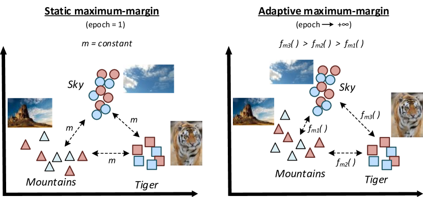
Figure 1. Adaptive margin constraints are scheduled to be progressively activated during the training phase.

In this paper we propose an adaptive neural structuring cross-modal subspace learning model (SAM), that dynamically organises instances on the new subspace according to their semantic similarity and inter-category correlations. In particular the two main novelties of the proposed method are:

• Adaptive margin constraints: we part ways with state-of-the-art methods based on the hinge-loss function with a constant margin $m$ between different categories, and introduce a novel adaptive margin function $f_{m}(\cdot)$ that infers the margin constraints during training.

• Scheduled activation of adaptive margins: by considering the incremental learning behaviour of neural architectures (Goodfellow et al., 2016), we propose a novel scheduled learning algorithm that progressively increases the parameters’ degrees of freedom to allow a shift from coarse-grain (fixed margin $m$) to fine-grain (adaptive margins $f_{m}(\cdot)$) training, as the model converges to a stable solution. Figure 1 illustrates this shift from epoch 1 to epoch t.

These contributions stem from the fact that the hinge-loss function does not adapt the constraints imposed by looking at the current subspace organisation, (e.g. clusters formed), at each training epoch $t$. We posit that semantic information used for subspace structuring should be directly incorporated in the ranking loss formulation, instead of adding extra terms to the main loss function. At the same time, the loss function should adapt the constraints imposed, at each training epoch, according to the current subspace structure and enforce semantic clusters formation, i.e. promote grouping of instances of the same semantic category.

In summary, we formulate an adaptive maximum-margin model, which dynamically adapts subspace structuring constraints over triplets, by jointly using semantic similarity and subspace category clusters enforcement rules to obtain an effective semantic subspace organisation. Experiments on three cross-modal retrieval benchmark datasets, where we compare our method with a considerable number of existing methods, reveal that our model is highly effective, outperforming state-of-the-art works.

2. Related work

Cross-modal subspace learning. Learning cross-modal embeddings, between visual and textual data, has been an active research topic (Rasiwasia et al., 2010; Feng et al., 2014; Yan and Mikolajczyk, 2015; Fan et al., 2017; Peng et al., 2018; Wang et al., 2017). In a pioneering work (Rasiwasia et al., 2010), Canonical Correlation Analysis (Hotelling, 1936) (CCA) was used to learn linear projections for each modality, by learning a set of canonical coefficients, that define a subspace where modalities are maximally correlated. This approach was extended for the multi-label scenario, by using label information to establish correspondences between instances (Ranjan et al., 2015). A multi-view kernel CCA formulation is proposed in (Gong et al., 2014), where a joint space for visual, textual and semantic information is learned.

Lately, neural methods have proved to be highly effective at learning non-linear projections that capture complex non-linear correlations. The loss function definition is generally the core component, for which several variants have been proposed. Deep Canonical Correlation Analysis (DCCA) was adopted in (Yan and Mikolajczyk, 2015) to match images and text, using non-linear projections. DCCA is a non-linear version of CCA that exploits the fact that the CCA objective function can be formulated based on a matrix trace norm, allowing for gradient-based optimisation. In (Feng et al., 2014) a neural architecture, the Correlation Autoencoder (Corr-AE), with two uni-modal autoencoders (one per modality) is used, enforcing correlation between learned hidden-representations. Instead of solely focusing in pairwise visual-textual correlations, in (Peng et al., 2016) extra constraints are added over inter-modal sample relations. Recently, in (Peng et al., 2018) authors model intra and inter-modality correlations, to unveil complex and fine-grain modality interactions. An adversarial approach is proposed in (Wang et al., 2017), where a common subspace is learned by a mini-max game between a feature projector and a modality classifier. An effective approach, common to several state-of-the-art approaches is triplet ranking loss (Schroff et al., 2015), in which different triplet mining strategies may be devised.

Subspace structuring constraints. Apart from maximising correlation between different modalities, additional constraints are usually added to the global loss function. In (Kang et al., 2017) center-loss is used to minimise intra-category invariance, under a metric learning approach. A successful approach consists of combining intra-modality semantic category and inter-modality pairwise similarity constraints (Wang et al., 2016b; Peng et al., 2018; Wang et al., 2017). Such constraints are commonly enforced over sampled triplets. In (Wang et al., 2016b) structure-preserving (hinge loss based) constraints with fixed margins, are used to push semantically similar instances closer to each other. In this paper, we follow a similar intuition, but instead we adaptively change the margin during training to enforce a per-category cluster formation and preservation.

Maximum-margin learning. To organise data by their semantic correlations, ranking loss is a widely adopted approach for cross-modal subspace learning due to its effectiveness (Wu et al., 2017; Wang et al., 2017). A set of similarity constraints are formulated under the hinge-loss, enforcing the similarity of positive instances to be far apart from similarity of negative ones, by at least a margin $m$. In state-of-the-art works, this margin is fixed with a constant value for all categories. In fact, this corresponds to a relaxation of the subspace structuring problem, in which the embedding’s semantic similarities are neglected, thus possibly sacrificing optimal data organisation. Following this line of reasoning, Li et al. (2015) replace the margin by the mean per joint error function, and in (Wu et al., 2017) the margin is replaced by the correlation of categories in the original feature space. We depart from the above methods by proposing an adaptive maximum-margin formulation that infers margin values during training.

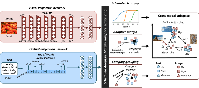
Figure 2. SAM model architecture. The model is composed by two sub-networks coupled by the loss function $\mathcal{L}_{SAM}$. At each learning epoch $t$ the loss $\mathcal{L}_{SAM}$ imposes triplet-specific constraints, enforcing cluster formation/preservation and organising instances according to their semantic similarity.

3. Cross-modal subspace structuring

3.1. Definitions

Let $\mathcal{C}$ be a corpus of multimodal instances, where without loss of generality, the visual (images) and textual modalities are considered. Each instance $d^{i}\in\mathcal{C}$ is defined as $d^{i}=(x_{V}^{i},x_{T}^{i},l^{i})$, where $x_{V}^{i}\in\mathbb{R}^{D_{V}}$ and $x_{T}^{i}\in\mathbb{R}^{D_{T}}$ are the instance’s image $d_{V}^{i}$ and text $d_{T}^{i}$ feature representations, respectively, and $l^{i}\in L$ the instance category. $L$ is the set of semantic categories. Let $*\in\{V,T\}$ on the remainder of this paper, to avoid notation cluttering.

In cross-modal subspace learning, the goal is to learn a subspace in which instances’ textual and visual elements, of the same semantic category, will be maximally correlated. The original feature spaces of $x_{V}$ and $x_{T}$ are dissimilar and cannot be used to perform cross retrieval, as they not only may have different dimensionalty but also encode different characteristics and semantics. To this end, for each original modality space, the goal is to learn the projections:

(1) $$\mathcal{P}_{\theta_{V}}(\cdot):\mathbb{R}^{D_{V}}\mapsto\mathbb{R}^{D}\hskip 28.45274pt\mathcal{P}_{\theta_{T}}(\cdot):\mathbb{R}^{D_{T}}\mapsto\mathbb{R}^{D}$$

mapping images $x_{V}$ and texts $x_{T}$ to a common cross-modal subspace, with dimensionality $D$. Similarity between two $\ell_{2}$ normalised projected sample modalities $x^{i}_{*}$ and $x^{j}_{*}$, is defined as cosine similarity, and efficiently computed based on a dot product $s(x^{i}_{*},x^{j}_{*})=\mathcal{P}_{\theta_{*}}(x^{i}_{*})\cdot\mathcal{P}_{\theta_{*}}(x^{j}_{*})$, with the function $s(\cdot,\cdot)$, mapping to the range $[-1,1]$.

3.2. Adaptive subspace learning

Modality projections into cross-modal subspaces must capture both inter-category and inter-modality correlations in that subspace. To this end, the cross-modal subspace learning problem is commonly formulated using a maximum-margin learning approach, by imposing a set of constraints over pairwise instance’s similarity, on the target subspace (Yao et al., 2015; Wang et al., 2016b, 2017; Semedo and Magalhaes, 2018; Peng et al., 2018).

For an anchor instance $x_{*}^{a}$, such constraints enforce the similarity of positive instances $s(x_{*}^{a},x_{*}^{p})$, i.e. sharing one category $l\in L$, to be higher than the similarity of negative samples $s(x_{*}^{a},x_{*}^{n})$, i.e. not sharing a category, by at least a margin $m$. This constraint is formulated as:

(2) $$s(x_{*}^{a},x_{*}^{p})>s(x_{*}^{a},x_{*}^{n})+m.$$

The constraint above is then enforced over each pair of instances, resulting in a considerable large set of constraints. For training, such constraints are then relaxed using the hinge loss (Herbrich et al., 2000).

3.2.1. Static maximum-margin formulation

We start by formulating a loss function $\mathcal{L}$, under this framework, by imposing maximum-margin constraints over the two modality directions ($image\mapsto text$ and $text\mapsto image$), thus simultaneously capturing inter-modality and inter-category correlations. Namely, at every training epoch $t$, given triplets of the form $(x_{*}^{a},x_{*}^{p},x_{*}^{n})$, where $x_{*}^{p}$ and $x_{*}^{n}$ stand for positive and negative instances, respectively, w.r.t. an anchor $x_{*}^{a}$, we compute the model loss,

(3) $$\begin{split}\mathcal{L}(t,\theta)&=\sum_{p,n}\underbrace{max(0,m-s(x_{V}^{a},x_{T}^{p})+s(x_{V}^{a},x_{T}^{n}))}_{image\ \mapsto\ text}\ \ +\\ &\ \ \ \ \sum_{p,n}\underbrace{max(0,m-s(x_{T}^{a},x_{V}^{p})+s(x_{T}^{a},x_{V}^{n}))}_{text\ \mapsto\ image},\end{split}$$

where $m$ denotes the margin and $\theta$ the model parameters. Note that unlike other cross-modal subspace learning works (Peng et al., 2018; Wang et al., 2017; Wu et al., 2017), the positive instance $x_{*}^{p}$ from each triplet is only the opposite modality of the same instance $d^{i}$, i.e. $x_{V}^{p}=x_{V}^{a}$ or $x_{T}^{p}=x_{T}^{a}$. A negative sampling strategy is then applied to mine triplets that respect these conditions.

3.2.2. Adaptive maximum-margin formulation

The maximum-margin formulation defined in eq. 3 assumes that any two instances from different categories are equally correlated. This is reflected by the adoption of a constant margin $m$.

Inspired by maximum-margin structured SVM (Tsochantaridis et al., 2005) formulation, we propose to (1) incorporate inter-category semantic correlations into the subspace structuring and (2) guide the projection learning algorithm, at each epoch, with structure preserving constraints that are derived from the current state of the subspace. To achieve this, we propose an adaptive margin formulation, defined by a non-negative margin function $f_{m}(d^{a},d^{n},t)$, where $d^{a}$ and $d^{n}$ correspond to semantically different instances (i.e. belong to different categories) and $t$ denotes the current epoch of the subspace training algorithm. The margin constraints, for every instance pair, at epoch $t$, are then reformulated as:

(4) $$s(x_{*}^{a},x_{*}^{p})>s(x_{*}^{a},x_{*}^{n})+f_{m}(d^{a},d^{n},t).$$

The rationale enclosed in this formulation is that for each pair of instances of different categories, $f_{m}(\cdot)$ outputs a margin that encodes the degree of separation between the considered categories. On every epoch $t$, the margin is linked to the pairwise correlation of the instances’ original feature vectors and current subspace structure. Accordingly, the adaptive subspace learning loss function $\mathcal{L}_{SAM}$, at epoch $t$ becomes:

(5) $$\begin{split}&\mathcal{L}_{SAM}(t,\theta)=\\ &\ \sum_{p,n}\underbrace{max(0,f_{m}(d^{a},d^{n},t)-s(x_{V}^{a},x_{T}^{p})+s(x_{V}^{a},x_{T}^{n}))}_{image\ \mapsto\ text}\ \ +\\ &\ \sum_{p,n}\underbrace{max(0,f_{m}(d^{a},d^{n},t)-s(x_{T}^{a},x_{V}^{p})+s(x_{T}^{a},x_{V}^{n}))}_{text\ \mapsto\ image}.\end{split}$$

Similarly to maximum margin methods, this formulation guides the model towards incorporating semantic information, regarding intra-category pairwise correlations. However, we observe that the difference of the similarities between positive and negative instances are, on average, inter-category specific. Therefore, we account for the current subspace organisation (at each epoch $t$), to decide what should be the magnitude of the margin, i.e. $f_{m}$.

3.3. Scheduled activation of adaptive margins

For neural subspace learning, in the first gradient updates, the subspace organisation is expected to be highly volatile, constantly changing at each epoch. It follows that for neural networks trained using stochastic gradient descent, it is not trivial to estimate beforehand when (i.e. at each epoch) is the model about to converge. Thus, we propose an approximation strategy that imposes a hard (i.e. a static high magnitude) margin on all triplet constraints on the first few epochs. This allows the model to find an initial coarse organisation of the subspace. Then, as the number of epochs progress, the static constraints give way to triplet specific constraints, that better capture the fine-grain interactions among instances.

Inspired by adaptive strategies for neural network training, such as the Adam (Kingma and Ba, 2014) optimiser, which schedules different learning rates, we propose a smoothed scheduled shift function from static to an adaptive maximum-margin formulation, as the training algorithm converges (Figure 3). To this end, a scheduled adaptive margin function $f_{m}$ is defined as:

(6) $$\begin{gathered}f_{m}(d^{a},d^{n},t)=\alpha(t)\cdot f_{am}(d^{a},d^{n},t)+(1-\alpha(t))\cdot m\\ \text{s.t. }\ \ \alpha(t)=\frac{1}{1+e^{-k\cdot(t-f_{a}\cdot n_{e})}},\end{gathered}$$

where the $\alpha(t)$ is a scheduler function, defined as a compressed sigmoid, that gradually activates the adaptive margin, according to the current epoch $t$. The $\alpha(t)$ function is defined by a smoothing term $k$, the total number of epochs $n_{e}$ and an activation factor $f_{a}\in[0,1]$. Figure 3 illustrates how each parameter is used to define $\alpha(t)$.

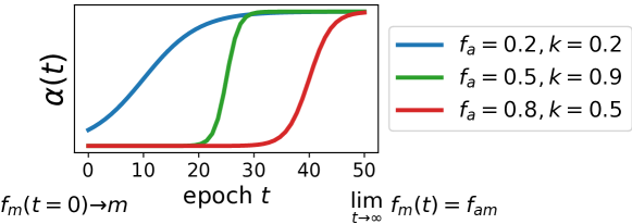
Figure 3. Plot of $\alpha(t)$ with $n_{e}=50$. The scheduling training enables a smooth transition from static margins to adaptive margins. Best viewed in color.

3.4. Adaptive margin function definition

In this section we describe how the adaptive margin function $f_{am}(d^{a},d^{n},t)$ is materialised. We formulate $f_{am}$ such that it implements an adaptive margin, encoding: a) the semantic correlation – estimated from original modality features – between instances from different categories, and b) cluster formation enforcement, for each semantic category, according to the epoch $t$ of the algorithm. Figure 2 illustrates $f_{am}$ components. In particular, we define the adaptive margin function as

(7) $$f_{am}(d^{a},d^{n},t)=\lambda\cdot f_{ms}(d^{a},d^{n})+(1-\lambda)\cdot f_{mc}(d^{a},d^{n},t),$$

where $f_{ms}$ quantifies semantic correlation, and $f_{mc}$ the similarity between category clusters at epoch $t$, of two instances $d^{a}$ and $d^{n}$. The parameter $\lambda$ models the trade-off between the two components.

Semantic inter-category pairwise correlations. From a semantic standpoint, pairwise correlations across categories, will be different (e.g. instances from category sky are expected to be more correlated with instances from clouds than from flowers). In our neural subspace structuring model, the function $f_{ms}$ accounts for such semantic correlations by evaluating similarity on each modality original spaces. The function $f_{ms}$ is then defined as:

(8) $$\begin{split}f_{ms}(d^{a},d^{n})=\frac{||x^{i}_{V}-x^{n}_{V}||_{2}+||x^{i}_{T}-x^{n}_{T}||_{2}}{2}.\end{split}$$

From the definition, $f_{ms}$ averages the semantic similarity of both visual and textual modalities, extracted from the modalities’ original feature space. The output of this function is normalized to $[0,1]$.

Category cluster formation and preservation. Given a randomly initialised neural network model, it can converge to different local optima, thus resulting in different subspace organisation. From this observation, we pose that for near convergence epochs, it is important to restrict model updates, preserving currently formed category clusters and forcing instances to move towards their category cluster. As a generalization, the centroid of a given category $l$ is computed as:

(9) $$\begin{split}\mathcal{P}_{*c}(l,t)=\frac{1}{|\{x^{j}_{*}:l^{j}=l\}|}\cdot\sum_{x^{k}_{*}\in\{x^{j}_{*}:l^{j}=l\}}\mathcal{P}_{\theta_{*}}(x_{*}^{k};t),\end{split}$$

To materialise the described behaviour, we rely on the cosine distance $d$ to define $f_{mc}$ as:

(10) $$\begin{split}&f_{mc}(d^{a},d^{n},t)=\\ &\frac{1}{2}\cdot\big{[}d(\mathcal{P}_{Vc}(l^{a},t),\mathcal{P}_{Vc}(l^{n},t))+d(\mathcal{P}_{Tc}(l^{a},t),\mathcal{P}_{Tc}(l^{n},t))\big{]},\end{split}$$

where for a given category $l$, $\mathcal{P}_{Vc}(l,t)$ and $\mathcal{P}_{Tc}(l,t)$ denote the centroid of the visual and textual projections, at epoch $t$. $d$ stands for the cosine distance $1-s(\cdot,\cdot)$, with $s$ being normalised a priori to $[0,1]$ range. Essentially, given a pair of instances, $f_{mc}$ evaluates the distance between the corresponding category centroids, for both visual and textual projections. Grounding the margin on $f_{mc}$ simultaneously enforces cluster formation and preservation. This is achieved because during training, the function $f_{mc}$ will simultaneously attempt to preserve the current subspace organisation and push bad aligned projections towards the corresponding category centroid.

3.5. Neural architecture

To learn projections $\mathcal{P}_{\theta_{V}}(\cdot)$ and $\mathcal{P}_{\theta_{T}}(\cdot)$, we consider a two decoupled network architecture, to learn non-linear mappings, predominant across multiple state-of-the-art works (Ngiam et al., 2011; Fan et al., 2017; Wang et al., 2017; Yan and Mikolajczyk, 2015; Feng et al., 2014). The networks are jointly trained by a common loss function $\mathcal{L}_{SAM}$. For each modality, a feedforward network $f_{*}$ maps original modality representations onto $\mathcal{S}$, comprising 2 fully connected layers (with dimensions 1024 and $D$, respectively) and $tanh$ non-linearities. For semantically rich image feature representation, each $x_{V}^{i}$ is obtained from a pre-trained CNN. Each $x_{T}^{i}$ is represented as a bag-of-words vector. Then, $f_{*}$ takes its corresponding modality as input: $d_{V}^{i}$ RGB image for $f_{V}$ and $d_{T}^{i}$ bag-of-words text representation for $f_{T}$. Figure 2 depicts the full architecture.

3.6. Training and inference

We jointly learn both the cross-modal projections $\mathcal{P}_{\theta_{V}}(\cdot)$ and $\mathcal{P}_{\theta_{T}}(\cdot)$, while adaptively performing neural subspace structuring, by minimising the function:

(11) $$\begin{gathered}\operatorname*{arg\,min}_{\theta_{V},\theta_{T}}\mathcal{L}_{SAM}(\theta_{V},\theta_{T})\end{gathered}$$

where $\mathcal{L}_{SAM}$ adaptively organizes instances according to their inter-category and inter-modal correlations. Pseudocode is illustrated in algorithm 1. A stochastic sampling strategy is adopted, in which to evaluate $\mathcal{L}_{SAM}(\theta_{V},\theta_{T})$, negative samples are sampled directly from mini-batches. At each epoch, all samples are seen by the network. This approach severely reduces the model complexity, while still achieving convergence. The whole model is then optimised using Stochastic Gradient Descent.

Algorithm 1 Pseudocode for SAM optimisation.

0:  Corpus $\mathcal{C}=\{d^{1},\ldots,d^{n}\}$ of multimodal instances, with $d^{i}=(x^{i}_{V},x^{i}_{T},l^{i})$;Initialise network weights: $\theta_{V},\theta_{T}$;Hyperparameters: $\lambda$, $k$, $f_{a}$, subspace dimensionality $D$, learning rate $\eta$, mini-batch size $b$;

1:  repeat until convergence:    

2:  for $t$ epochs do

3:        Sample mini-batch to create triplets of the form $(x_{V}^{i},x_{T}^{i},x_{T}^{n})$ and $(x_{T}^{i},x_{V}^{i},x_{V}^{n})$;

4:        Update $\theta_{V}$ and $\theta_{T}$ through BP, with stochastic gradients, using $\alpha(t)$:

5:        ${\theta_{V}}\leftarrow{\theta_{V}}-\eta\cdot{\nabla}_{\theta_{V}}\frac{1}{b}\left(\mathcal{L}_{SAM}\right)$;

6:        ${\theta_{T}}\leftarrow{\theta_{T}}-\eta\cdot{\nabla}_{\theta_{T}}\frac{1}{b}\left(\mathcal{L}_{SAM}\right)$;

7:        Update the weight of the adaptive margin:

8:        $\alpha(t+1)\leftarrow\frac{1}{1+e^{-k\cdot((t+1)-f_{a}\cdot n_{e})}}$;

9:  end for

10:  return  projection networks, $\mathcal{P}_{\theta_{V}}(\cdot)$ and $\mathcal{P}_{\theta_{T}}(\cdot)$.

4. Evaluation

4.1. Datasets

We evaluate our proposed methods in three widely used cross-modal retrieval benchmark datasets.

Wikipedia (Rasiwasia et al., 2010). Comprised by a total of 2,866 visual-textual pairs, extracted from Wikipedia’s "featured articles", where each article is accompanied by a single image. Each article is annotated with 10 semantic categories. We split the dataset following (Rasiwasia et al., 2010; Feng et al., 2014; Peng et al., 2016), with 2,173 instances for training, 231 for validation, and 462 for testing.

NUS-WIDE (Chua et al., 2009). The NUS-WIDE dataset is comprised by a total of 269,648 instances (images and corresponding tags), from the Flickr network, annotated with one or more categories from a total of 81 distinct semantic categories. For comparison, we follow the protocol of Peng et al. (2018): only instance pairs that belong to a single category are kept and the instances from the 10 categories with more instances are chosen. This results in more than 60,000 instances. Splits are created following (Peng et al., 2018), resulting in 23,661 instances for testing, 5,000 for validation and the remaining for training.
NUS-WIDE-10K is a subset of NUS-WIDE created by strictly following the protocol of (Feng et al., 2014): the 10 categories with more instances are chosen, and for each category, 1000 instances are sampled. Only pairs that belong to a single category are considered. Three splits, equally balanced w.r.t. to number of instances per category, are sampled randomly: 8,000 instances for training, 1,000 for validation and 1,000 for testing.

Pascal Sentence (Rashtchian et al., 2010). Comprised by 1,000 visual-textual pairs, from the 2008 PASCAL development kit, categorised within 20 categories, with instances evenly distributed across categories. We follow (Feng et al., 2014; Peng et al., 2016) and randomly and evenly split the dataset with 800 instances for training, 100 for validation and 100 for testing.

4.2. Methodology

We evaluate the retrieval performance using mean Average Precision ($mAP$), which is the standard evaluation metric for cross-modal retrieval (Rasiwasia et al., 2010; Wang et al., 2016c; Feng et al., 2014; Wang et al., 2017; Yan and Mikolajczyk, 2015; Peng et al., 2018). We follow (Rasiwasia et al., 2010; Kang et al., 2015; Zhai et al., 2014; Peng et al., 2018) and compute $mAP$ for all the retrieved results. For $mAP$, an instance is relevant if it has the same category. Two tasks are evaluated: 1) Image-to-Text retrieval ($I\mapsto T$) and 2) Text-to-Image ($T\mapsto I$) retrieval. Core parameters of SAM are analysed to assess their impact in the performance. Each $mAP$ result reported of our method corresponds to the average of 5 runs.

Table 1. mAP performance results across different datasets. The second half of the table concern deep-learning methods.

Method	Pascal Sentences			NUS-WIDE-10k			Wikipedia
	$I\mapsto T$	$T\mapsto I$	Avg	$I\mapsto T$	$T\mapsto I$	Avg	$I\mapsto T$	$T\mapsto I$	Avg
CCA (Hotelling, 1936)	0.203	0.208	0.206	0.167	0.181	0.174	0.298	0.273	0.286
CFA (Li et al., 2003)	0.476	0.470	0.473	0.406	0.435	0.421	0.319	0.316	0.318
KCCA (Hardoon et al., 2004)	0.488	0.446	0.467	0.351	0.356	0.354	0.438	0.389	0.414
LGCFL (Kang et al., 2015)	0.539	0.503	0.521	0.453	0.485	0.469	0.466	0.431	0.449
JRL (Zhai et al., 2014)	0.563	0.505	0.534	0.466	0.499	0.483	0.479	0.428	0.454
Corr-AE (Feng et al., 2014)	0.532	0.521	0.527	0.441	0.494	0.468	0.442	0.429	0.436
DCCA (Yan and Mikolajczyk, 2015)	0.568	0.509	0.539	0.452	0.465	0.459	0.445	0.399	0.422
CMDN (Peng et al., 2016)	0.544	0.526	0.535	0.492	0.542	0.517	0.487	0.427	0.457
Deep-SM (Wei et al., 2016)	0.560	0.539	0.550	0.497	0.478	0.488	0.478	0.422	0.450
ACMR (Wang et al., 2017)	0.538	0.544	0.541	0.519	0.542	0.531	0.468	0.412	0.440
CCL (Peng et al., 2018)	0.576	0.561	0.569	0.481	0.520	0.501	0.505	0.457	0.481
SAM ($\alpha(t)=1,\ \lambda=1$)	0.586	0.590	0.588	0.539	0.559	0.549	0.406	0.382	0.394
SAM	0.637	0.643	0.640	0.563	0.594	0.579	0.518	0.457	0.487

4.3. Implementation details

Networks are jointly trained using Stochastic Gradient Descent, with $0.9$ Nesterov momentum, and a learning rate $\eta=$5\text{\times}{10}^{-3}$$, with a decay of $1\text{\times}{10}^{-6}$. The model with lowest validation error is kept. Mini-batch size is set to $200$ for all datasets, and the total number of epochs is set to $100$. The projections dimension is set to $D=200$ and the margin $m=1.0$. For each neuron, tanh non-linearities are applied. Dropout with $p=0.1$ is applied to the first hidden layer. Images representations are obtained by feeding each individual image through a pre-trained VGG-19 (Simonyan and Zisserman, 2014) convolutional network, and extracting the output of the last fully connected layer (fc7). For texts, we adopt a BoW representation, with 1000-D vocabulary size for NUS-WIDE-10k and Pascal Sentences, and 3000-D for wikipedia.

4.4. Cross-modal retrieval

We compare our proposed approach, SAM, with a total of 11 state-of-the-art works, on the task of cross-modal retrieval. Namely, we compare against CCA (Hotelling, 1936), CFA (Li et al., 2003), KCCA (Hardoon et al., 2004), Corr-AE (Feng et al., 2014), JRL (Zhai et al., 2014), LGCFL (Kang et al., 2015), DCCA (Yan and Mikolajczyk, 2015), CMDN (Peng et al., 2016), Deep-SM (Wei et al., 2016), ACMR (Wang et al., 2017) and CCL (Peng et al., 2018).

Pascal sentences dataset. Table 1 shows the results obtained. Our method outperforms all the compared methods, on both $I\mapsto T$ and $T\mapsto I$ settings. Namely, SAM achieved a relative improvement of $\approx 12.5\%$, with respect to the second best performing method, CCL. CCL models intra-modality and inter-modality correlations through distinct constraints, using a strategy that balances both types of correlation constraints. These are then superseeded by a ranking loss function in which a static margin is used. Instead, SAM adopts an adaptive margin formulation, in which intra and inter modality correlations are directly modelled in a single constraint. The best result was achieved with $\lambda=0.25$, $f_{a}=0.4$ and $k=0.1$. SAM started smoothly activating the adaptive margin at about half the training epochs, revealing preference for starting using $f_{am}$ sooner. The semantic similarity component $f_{ms}$ plays an important role in organising the space. Notwithstanding, the component $f_{mc}$ has revealed to be the most important one ($75\%$), effectively guiding the subspace structuring.

NUS-WIDE-10k dataset. From the results on table 1, we can see that our method also achieved the best performance when compared to all methods, on both cross-modal retrieval directions. It outperformed both traditional cross-media models (top rows of table 1) and the most recent deep learning methods. With respect to the second best performing method, ACMR, which uses an adversarial approach for subspace learning, we obtain a relative improvement of $\approx 9\%$, on the average of $T\mapsto I$ and $I\mapsto T$. This confirms the importance of moving towards an adaptive margin formulation. The best result was obtained with $\lambda=0.05$, $f_{a}=0.9$ and $k=0.1$. Hence, in contrast to the results on the Pascal sentences dataset, the method started activating the adaptive margin near the last epochs of training. Moreover, once again, more importance was given to the cluster enforcement and preservation ($95\%$ of the weight). Our method obtains a high $mAP$ on both directions, but performs better on the $T\mapsto I$ direction. We believe that the reason is that visually, some categories have very similar content (e.g. sky vs. clouds). However, the text in this dataset correspond to tags, which due to the sparsity of BoW representation, turns out to have good discriminative properties.

Wikipedia dataset. As with the previous datasets, our method outperforms all the compared methods. On the Wikipedia dataset, categories are very broad (e.g. Art & Architecture, Media, etc.), with texts and images of the same category being highly diverse. Therefore, in this dataset, given the small amount of instances available for training, it is harder to align modalities. As this is reflected in original feature representations, the function $f_{ms}$, which organises instances according to semantic similarity on original features, ends up not helping structuring the space. Supporting this observation is the fact that the best result was obtained with $\lambda=0.05$. The category cluster formation and preservation, enforced by function $f_{mc}$ provides the major contribution to the effectiveness.

To further complement our evaluation, we also compare our method against CMOLRS (Wu et al., 2017), which formulated the margin as an original-feature driven margin that is fixed during training, i.e. using only a simplified version of $f_{ms}$ factor of SAM. On the Wikipedia dataset, CMOLRS achieved a mAP@100 of $0.413$ while SAM achieves a mAP@100 of $0.541$. As authors only report mAP@100, we did not included it in table 1. This confirms the importance of dynamically adjusting margin values during training and of the novel cluster formation and preservation component $f_{mc}$.

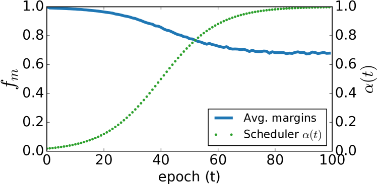
Figure 4. Global average adaptive margin $f_{m}$ over training epochs (t). The left y-axis corresponds to the $f_{m}$ value and the right y-axis to the scheduling function $\alpha(t)$ value.

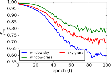
(a) Scheduled Adaptive Margins between 3 categories.

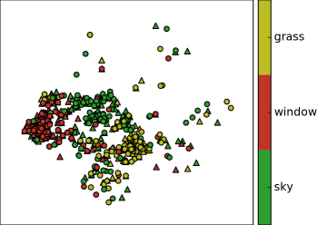
(b) t-SNE projections

Figure 5. Analysis of the margin values over each epoch (t), between three categories (left), versus final t-SNE model projections (right).

Large-scale NUS-WIDE. To further explore the generalisation of SAM algorithm, we evaluated SAM in the large-scale full NUS-WIDE dataset. Table 2 supports the same conclusions that where drawn from the previous analysis. It is also noticeable, that all models improved thanks to the larger training dataset.

Overview. In overall, our method has proven to be effective, outperforming previous state-of-the-art methods on all datasets. The cluster enforcement and preservation component ($f_{mc}$) proved to be crucial to achieve state-of-the-art performance. Unlike most methods, which impose extra constraints by augmenting a projection network by adding additional loss terms, our approach imposes those constraints by directly adapting the margin between instance pairs during training, thus resulting in a simpler but effective model.

By modelling the semantic inter-category pairwise correlations, our model is able to transfer semantic correlations from the original feature space directly to the common subspace. Then, by enforcing cluster formation after achieving a stable subspace organisation, our method improves significantly from state-of-the-art works.

Table 2. mAP results on the NUS-WIDE dataset.

	NUS-WIDE
Methods	$I\mapsto T$	$T\mapsto I$	Avg.
CCA (Hotelling, 1936)	0.244	0.275	0.260
CFA (Li et al., 2003)	0.358	0.361	0.360
KCCA (Hardoon et al., 2004)	0.348	0.481	0.415
LGCFL (Kang et al., 2015)	0.512	0.600	0.556
JRL (Zhai et al., 2014)	0.615	0.592	0.604
Corr-AE (Feng et al., 2014)	0.391	0.429	0.410
DCCA (Yan and Mikolajczyk, 2015)	0.475	0.500	0.488
CMDN (Peng et al., 2016)	0.643	0.626	0.635
CCL (Peng et al., 2018)	0.671	0.676	0.674
SAM	0.701	0.707	0.704

4.5. Scheduled adaptive margins analysis

In this section we examine behaviour of SAM by looking at the margin values imposed by the model on each triplet constraints, over each epoch (t).

4.5.1. Average margin values vs. scheduler function

The scheduler function $\alpha(t)$ shifts from a high-magnitude constant margin ($m=1$), to the adaptive margin $f_{am}$. To inspect this behaviour, we computed the average margin value, imposed to all triplets, on each epoch t, on the NUSWIDE-10k dataset. Figure 5 shows the average $f_{m}$ value (blue line) versus the scheduler function value $\alpha(t)$ (green line), over the training epochs. It can be observed that at each epoch, the average margin imposed by $f_{m}$ tends to be smaller. One can also observe that $\alpha(t)$ has a sigmoidal shape.

4.5.2. Average margin values for each Category

In order to provide a deeper understanding of what the model achieves, we show in Figure 5, also on the NUSWIDE-10k dataset, the average margin values between three pairs of categories at each training epoch t, and a projection of the final cross-modal subspace.

The scale of the average margin values in the last epoch ($t=100$), between each pair of the considered categories, is reflected in the obtained subspace. It is noteworthy to say that the magnitude of the value $m$ reflects the difference between similarities of pairs of instances, not distance on the subspace. Nevertheless, the magnitude of the values still allow to confirm its impact in the subspace organisation. For instance, in the plot on the left, it can be seen that in the last epochs, our model enforced an average margin of roughly $0.6$ between instances of category window versus category sky, which is much smaller than the value between instances of window and grass, which is roughly $0.77$. Looking at the t-SNE projections, we can actually see that the organisation of instances respects these values, with instances of category window being closer to instances of sky than to grass.

These experiments are crucial to understand the underpinnings of SAM: Figure 5 confirms that the average margin value gradually decreases during training, with triplet constraints over window-sky categories having lower magnitude margins than window-grass, thus reflecting visual and textual semantic similarity as intended.

Figure 6 delves into this question and shows the average margin value per category imposed by $f_{m}$, against triplets of the remaining categories, at each epoch $t$. Given the target category $c_{1}$ of each plot, each line corresponds to a category $c_{2}$. Namely, it corresponds to the average of the margin values, imposed by $f_{m}$, to triplets with the positive instance belonging to category $c_{1}$ and the negative belonging to category $c_{2}$. It is interesting to note that all margins are significantly different. In particular, categories grass and person are the ones with most homogenous margins. In contrast, categories sky and animal took full advantage of the scheduled adaptive margins and ended up with very different margins to all other categories.

4.5.3. Scheduler and $f_{mc}$ impact

The scheduler, together with the cluster formation and enforcement $f_{mc}$ component of the adaptive margin, are key novel components, responsible for achieving state-of-the-art performance. To confirm this, we evaluated SAM with the scheduler deactivated ($\alpha(t)=1)$ and with $f_{mc}$ disabled ($\lambda=1$). As can been seen from table 1, this results in a drop of performance of $\approx 8\%$, $\approx 5\%$ and $\approx 19\%$, on Pascal Sentences, NUS-WIDE-10k and Wikipedia, respectively, confirming the crucial importance of the scheduler and $f_{mc}$.

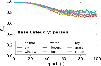
(a)

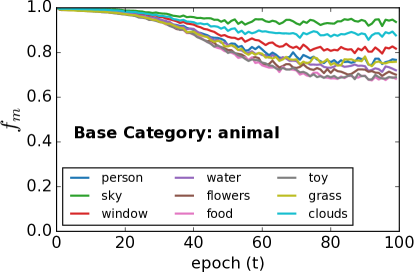
(b)

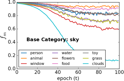
(c)

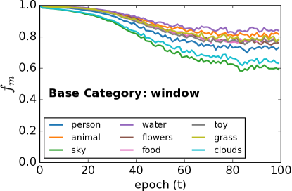
(d)

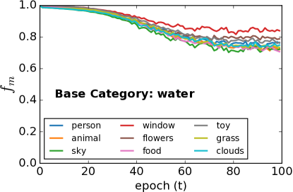
(e)

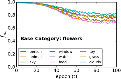
(f)

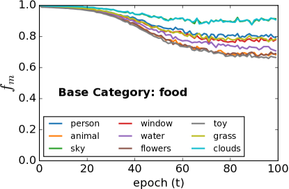
(g)

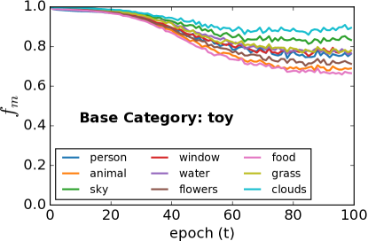
(h)

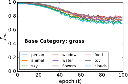
(i)

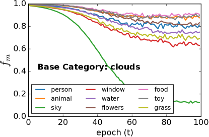
(j)

Figure 6. Average per-category margin for each category, at each training epoch (t). Average value of $f_{m}$ between every instance $d^{i}$, against all instances $d^{n}$ of other categories.

4.6. Analysis of activation phase

In this section we will analyse the impact of the activation phase $f_{a}$ and the semantic correlation vs. cluster enforcement trade-off $\lambda$ parameter. To do this, we measure the $mAP$ score on the Pascal Sentences dataset. Namely, we evaluate $f_{a}\in\{0.0.,0.2,0.4,0.6,0.8,1.0\}$ and $\lambda\in\{0.0,0.1,0.25,0.75,1.0\}$, fixing all the remaining parameters, and show the results in Figure 7. The $x$-axis represents the value of $f_{a}$ and the $y$-axis the $mAP$ score obtained. Each curve corresponds to a value of $\lambda$.

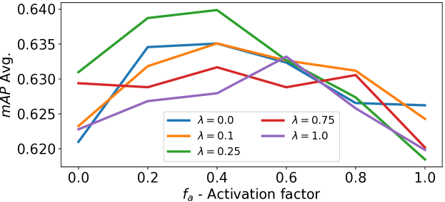
Figure 7. Parameter Analysis ($\lambda$ and activation function $f_{a}$) on Pascal Sentences dataset.

The first observation is that imposing the adaptive margin too early is bad. For instance, when $f_{a}$ is close to zero, the method starts using the adaptive margin from the beginning of the training, resulting in low performance. This confirms our intuition that in the first training iterations, the subspace is still coarsely organised. As the parameter $f_{a}$ increases, we can see that the results improve significantly, reaching a performance peak on $f_{a}=0.4$, for four of the five experimented values of $\lambda$. Namely, smoothly activating the adaptive margin with $f_{a}=0.4$, and giving around $75\%$ weight to $f_{mc}$ (cluster formation and preservation component) and the remaining to $f_{ms}$, leads to the best performance. For all values of $\lambda$, activating the adaptive margin too late leads to significant performance drops. This is due to the fact that by activating later, the network has more chances to overfit using a static margin. At this point, neither the cluster formation $f_{mc}$, nor the semantic correlations $f_{ms}$ components are able to improve the subspace organisation. Regarding the trade-off parameter $\lambda$, we observe the trend that cluster formation has a higher impact on achieving better performance than semantic correlation, with peak performance occurring when both components are active.

5. Conclusions

In this paper we described a novel method to learn cross-modal embeddings. The method introduces a scheduled activation of adaptive margins that allow for triplet specific margins. The key takeaways of the proposed method are:

• Adaptive margin constraints: our approach impose general constraints while training the model by adapting the margins between instance pairs. This overcomes the fact that using a unique margin for all pairs is insufficient to adequately structure the subspace.

• Effective learning of pair-specific margins: results show that adaptive margins deliver state-of-the-art results. This is further possible due to the pair-specific margins that are learned by the model as illustrated by experimental results.

• Scheduled learning: new neural-network training approach was introduced that progressively activates the adaptive margin function, through an epoch-aware scheduling strategy.

As future work, we plan to generalise adaptive ranking loss. Current results hint that the same principle can encode different constraints and thus be extended to other multimedia modelling tasks.

- (1)
- Chua et al. (2009) Tat-Seng Chua, Jinhui Tang, Richang Hong, Haojie Li, Zhiping Luo, and Yan-Tao Zheng. July 8-10, 2009. NUS-WIDE: A Real-World Web Image Database from National University of Singapore. In Proc. of ACM Conf. on Image and Video Retrieval (CIVR’09). Santorini, Greece.
- Fan et al. (2017) Mengdi Fan, Wenmin Wang, Peilei Dong, Liang Han, Ronggang Wang, and Ge Li. 2017. Cross-media Retrieval by Learning Rich Semantic Embeddings of Multimedia. In Proceedings of the 2017 ACM on Multimedia Conference (MM ’17). ACM, New York, NY, USA, 1698–1706. https://doi.org/10.1145/3123266.3123369
- Feng et al. (2014) Fangxiang Feng, Xiaojie Wang, and Ruifan Li. 2014. Cross-modal Retrieval with Correspondence Autoencoder. In Proceedings of the 22Nd ACM International Conference on Multimedia (MM ’14). ACM, New York, NY, USA, 7–16. https://doi.org/10.1145/2647868.2654902
- Gong et al. (2014) Yunchao Gong, Qifa Ke, Michael Isard, and Svetlana Lazebnik. 2014. A Multi-View Embedding Space for Modeling Internet Images, Tags, and Their Semantics. Int. J. Comput. Vision 106, 2 (Jan. 2014), 210–233. https://doi.org/10.1007/s11263-013-0658-4
- Goodfellow et al. (2016) Ian Goodfellow, Yoshua Bengio, and Aaron Courville. 2016. Deep Learning. The MIT Press.
- Hardoon et al. (2004) D. R. Hardoon, S. Szedmak, and J. Shawe-Taylor. 2004. Canonical Correlation Analysis: An Overview with Application to Learning Methods. Neural Computation 16, 12 (Dec 2004), 2639–2664. https://doi.org/10.1162/0899766042321814
- Herbrich et al. (2000) Ralf Herbrich, Thore Graepel, and Klaus Obermayer. 2000. Large Margin Rank Boundaries for Ordinal Regression. In Advances in Large Margin Classifiers, P. J. Bartlett, B. Schölkopf, D. Schuurmans, and A. J. Smola (Eds.). MIT Press, 115–132.
- Hotelling (1936) Harold Hotelling. 1936. Relations Between Two Sets of Variates. Biometrika 28, 3/4 (Dec. 1936), 321–377. https://doi.org/10.2307/2333955
- Huang et al. (2017) Xin Huang, Yuxin Peng, and Mingkuan Yuan. 2017. MHTN: Modal-adversarial Hybrid Transfer Network for Cross-modal Retrieval. CoRR abs/1708.04308 (2017). arXiv:1708.04308 http://arxiv.org/abs/1708.04308
- Kang et al. (2017) Cuicui Kang, Shengcai Liao, Zhen Li, Zigang Cao, and Gang Xiong. 2017. Learning Deep Semantic Embeddings for Cross-Modal Retrieval. In Proceedings of the Ninth Asian Conference on Machine Learning (Proceedings of Machine Learning Research), Min-Ling Zhang and Yung-Kyun Noh (Eds.), Vol. 77. PMLR, 471–486. http://proceedings.mlr.press/v77/kang17a.html
- Kang et al. (2015) C. Kang, S. Xiang, S. Liao, C. Xu, and C. Pan. 2015. Learning Consistent Feature Representation for Cross-Modal Multimedia Retrieval. IEEE Transactions on Multimedia 17, 3 (March 2015), 370–381. https://doi.org/10.1109/TMM.2015.2390499
- Kingma and Ba (2014) Diederik P. Kingma and Jimmy Ba. 2014. Adam: A Method for Stochastic Optimization. CoRR abs/1412.6980 (2014). arXiv:1412.6980 http://arxiv.org/abs/1412.6980
- Li et al. (2003) Dongge Li, Nevenka Dimitrova, Mingkun Li, and Ishwar K. Sethi. 2003. Multimedia Content Processing Through Cross-modal Association. In Proceedings of the Eleventh ACM International Conference on Multimedia (MULTIMEDIA ’03). ACM, New York, NY, USA, 604–611. https://doi.org/10.1145/957013.957143
- Li et al. (2015) Sijin Li, Weichen Zhang, and Antoni B. Chan. 2015. Maximum-Margin Structured Learning with Deep Networks for 3D Human Pose Estimation. In 2015 IEEE International Conference on Computer Vision, ICCV 2015, Santiago, Chile, December 7-13, 2015. IEEE Computer Society, 2848–2856. https://doi.org/10.1109/ICCV.2015.326
- Ngiam et al. (2011) Jiquan Ngiam, Aditya Khosla, Mingyu Kim, Juhan Nam, Honglak Lee, and Andrew Y. Ng. 2011. Multimodal Deep Learning. In Proceedings of the 28th International Conference on International Conference on Machine Learning (ICML’11). Omnipress, USA, 689–696. http://dl.acm.org/citation.cfm?id=3104482.3104569
- Peng et al. (2016) Yuxin Peng, Xin Huang, and Jinwei Qi. 2016. Cross-media Shared Representation by Hierarchical Learning with Multiple Deep Networks. In Proceedings of the Twenty-Fifth International Joint Conference on Artificial Intelligence (IJCAI’16). AAAI Press, 3846–3853. http://dl.acm.org/citation.cfm?id=3061053.3061157
- Peng et al. (2018) Y. Peng, J. Qi, X. Huang, and Y. Yuan. 2018. CCL: Cross-modal Correlation Learning With Multigrained Fusion by Hierarchical Network. IEEE Transactions on Multimedia 20, 2 (Feb 2018), 405–420. https://doi.org/10.1109/TMM.2017.2742704
- Ranjan et al. (2015) V. Ranjan, N. Rasiwasia, and C. V. Jawahar. 2015. Multi-label Cross-Modal Retrieval. In 2015 IEEE International Conference on Computer Vision (ICCV). 4094–4102. https://doi.org/10.1109/ICCV.2015.466
- Rashtchian et al. (2010) Cyrus Rashtchian, Peter Young, Micah Hodosh, and Julia Hockenmaier. 2010. Collecting Image Annotations Using Amazon’s Mechanical Turk. In Proceedings of the NAACL HLT 2010 Workshop on Creating Speech and Language Data with Amazon’s Mechanical Turk (CSLDAMT ’10). Association for Computational Linguistics, Stroudsburg, PA, USA, 139–147. http://dl.acm.org/citation.cfm?id=1866696.1866717
- Rasiwasia et al. (2010) Nikhil Rasiwasia, Jose Costa Pereira, Emanuele Coviello, Gabriel Doyle, Gert R.G. Lanckriet, Roger Levy, and Nuno Vasconcelos. 2010. A New Approach to Cross-modal Multimedia Retrieval. In Proceedings of the 18th ACM International Conference on Multimedia (MM ’10). ACM, New York, NY, USA, 251–260. https://doi.org/10.1145/1873951.1873987
- Schroff et al. (2015) Florian Schroff, Dmitry Kalenichenko, and James Philbin. 2015. FaceNet: A Unified Embedding for Face Recognition and Clustering. arXiv e-prints, Article arXiv:1503.03832 (March 2015), arXiv:1503.03832 pages. arXiv:cs.CV/1503.03832
- Semedo and Magalhaes (2018) David Semedo and Joao Magalhaes. 2018. Temporal Cross-Media Retrieval with Soft-Smoothing. In 2018 ACM Multimedia Conference on Multimedia Conference (MM ’18). ACM, New York, NY, USA, 1038–1046. https://doi.org/10.1145/3240508.3240665
- Simonyan and Zisserman (2014) Karen Simonyan and Andrew Zisserman. 2014. Very Deep Convolutional Networks for Large-Scale Image Recognition. CoRR abs/1409.1556 (2014). arXiv:1409.1556 http://arxiv.org/abs/1409.1556
- Tsochantaridis et al. (2005) Ioannis Tsochantaridis, Thorsten Joachims, Thomas Hofmann, and Yasemin Altun. 2005. Large Margin Methods for Structured and Interdependent Output Variables. J. Mach. Learn. Res. 6 (Dec. 2005), 1453–1484. http://dl.acm.org/citation.cfm?id=1046920.1088722
- Wang et al. (2017) Bokun Wang, Yang Yang, Xing Xu, Alan Hanjalic, and Heng Tao Shen. 2017. Adversarial Cross-Modal Retrieval. In Proceedings of the 2017 ACM on Multimedia Conference (MM ’17). ACM, New York, NY, USA, 154–162. https://doi.org/10.1145/3123266.3123326
- Wang et al. (2016a) K. Wang, R. He, L. Wang, W. Wang, and T. Tan. 2016a. Joint Feature Selection and Subspace Learning for Cross-Modal Retrieval. IEEE Transactions on Pattern Analysis and Machine Intelligence 38, 10 (Oct 2016), 2010–2023. https://doi.org/10.1109/TPAMI.2015.2505311
- Wang et al. (2016c) Kaiye Wang, Qiyue Yin, Wei Wang, Shu Wu, and Liang Wang. 2016c. A Comprehensive Survey on Cross-modal Retrieval. CoRR abs/1607.06215 (2016).
- Wang et al. (2016b) L. Wang, Y. Li, and S. Lazebnik. 2016b. Learning Deep Structure-Preserving Image-Text Embeddings. In 2016 IEEE Conference on Computer Vision and Pattern Recognition (CVPR). 5005–5013. https://doi.org/10.1109/CVPR.2016.541
- Wei et al. (2016) Yunchao Wei, Yao Zhao, Canyi Lu, Shikui Wei, Luoqi Liu, Zhenfeng Zhu, and Shuicheng Yan. 2016. Cross-Modal Retrieval With CNN Visual Features: A New Baseline. IEEE Transactions on Cybernetics (2016).
- Wu et al. (2018) Yiling Wu, Shuhui Wang, and Qingming Huang. 2018. Learning Semantic Structure-preserved Embeddings for Cross-modal Retrieval. In Proceedings of the 26th ACM International Conference on Multimedia (MM ’18). ACM, New York, NY, USA, 825–833. https://doi.org/10.1145/3240508.3240521
- Wu et al. (2017) Y. Wu, S. Wang, W. Zhang, and Q. Huang. 2017. Online low-rank similarity function learning with adaptive relative margin for cross-modal retrieval. In 2017 IEEE International Conference on Multimedia and Expo (ICME). 823–828. https://doi.org/10.1109/ICME.2017.8019528
- Xu et al. (2018) Xing Xu, Jingkuan Song, Huimin Lu, Yang Yang, Fumin Shen, and Zi Huang. 2018. Modal-adversarial Semantic Learning Network for Extendable Cross-modal Retrieval. In Proceedings of the 2018 ACM on International Conference on Multimedia Retrieval (ICMR ’18). ACM, New York, NY, USA, 46–54. https://doi.org/10.1145/3206025.3206033
- Yan and Mikolajczyk (2015) F. Yan and K. Mikolajczyk. 2015. Deep correlation for matching images and text. In 2015 IEEE Conference on Computer Vision and Pattern Recognition (CVPR). 3441–3450. https://doi.org/10.1109/CVPR.2015.7298966
- Yao et al. (2015) T. Yao, T. Mei, and C. W. Ngo. 2015. Learning Query and Image Similarities with Ranking Canonical Correlation Analysis. In 2015 IEEE International Conference on Computer Vision (ICCV). 28–36. https://doi.org/10.1109/ICCV.2015.12
- Zhai et al. (2014) X. Zhai, Y. Peng, and J. Xiao. 2014. Learning Cross-Media Joint Representation With Sparse and Semi-supervised Regularization. IEEE Transactions on Circuits and Systems for Video Technology 24, 6 (June 2014), 965–978. https://doi.org/10.1109/TCSVT.2013.2276704