Constructing Semi-Directed Level-1 Phylogenetic Networks from Quarnets

Abstract

We introduce two algorithms for reconstructing semi-directed level-1 phylogenetic networks from their complete set of 4-leaf subnetworks, known as quarnets. The first algorithm, the sequential method, begins with a single quarnet and adds on one leaf at a time until all leaves have been placed. The second algorithm, the cherry-blob method, functions similarly to cherry-picking algorithms for phylogenetic trees by identifying exterior network structures from the quarnets.

1 Introduction

Phylogenetics is the study of evolutionary relationships between species. A phylogenetic tree represents extant species as leaves and extinct species as internal vertices. Trees have a single path between any two vertices, which makes them insufficient for modeling evolutionary events such as hybridization or gene flow where lineages necessarily cross dagan2011phylogenomic . Phylogenetic networks allow for reticulation events which create underlying cycles on the graph. Thus network models may capture a more diverse collection of biological processes.

Edges of phylogenetic networks represent evolutionary change. In practice, it may be challenging to infer the direction of an evolutionary change from sequence data. In the recent work of Gross and Long, they show that under the Jukes-Cantor model, only the semi-directed structure of a 4-leaf network is identifiable gross . In a semi-directed network, all edges are undirected except for the edges that form a reticulation event where two lineages merge to form a single lineage. This limits, but does not explicitly identify, a possible root of the underlying network. Unrooted, semi-directed networks are the focus of this article.

Since the class of networks with $n$ leaves is infinite, most work in phylogenetic networks assumes that the model networks have a particular structure. The level of a phylogenetic network is the maximum number of reticulation events in any biconnected component of the network jansson2006inferring . We use the term level-$k$ networks to refer to all networks of the level at most $k$. Thus level-1 networks, which are our primary focus, include the set of phylogenetic trees. In this setting, we introduce two methods for building more extensive networks from smaller networks.

4-leaf trees, or quartets, have been used as building blocks for tree reconstruction astral ; Maxcut . Quartets are also beginning to play a role in network reconstruction. For instance, SNaQ reconstructs phylogenetic networks from the set of quartets displayed by a collection of gene trees snaq . Other work uses quartets to directly infer unrooted networks gambette2012quartets . Another approach focuses on quarnets, or 4-leaf networks. One such method focuses on undirected topologies and builds networks via a “blow up” method Huber2018 . None of these methods address semi-directed networks.

We develop two approaches for semi-directed network reconstruction, which allow for cycles of any size. These methods take the complete set of semi-directed quarnets displayed by a network and output the associated level-1 network. The first method is based on sequentially adding leaves to an existing network and can be viewed as a generalization of quartet-puzzling qtetpuzzling . The second algorithm, which we call the cherry-blob algorithm is a generalization of cherry picking on trees cherrypicking2 , where we recursively identify the external structures of a network which can include both tree cherries and also cycles in a level-1 network.

In Section 2 we introduce definitions and notation. Then, we present two building algorithms in Section 3 and Section 4. Finally, in Section 5, we discuss possible extensions of these algorithms when one does not have access to the complete set of displayed quarnets.

2 Background

Where possible, we adapt our network language and notation from gross . A network $N=(V,E)$ is a collection of vertices $V$ and set of unordered pairs of vertices that make up edge set $E$. We restrict our attention to networks which are finite, connected, and do not have self-loops or multiple edges between vertices. All degree 1 vertices are leaves of which there are $n$. We refer to the leaf set of a network $N$ as $X$ or alternatively as the support of $N$ denoted $supp(N)$.

On a network, a reticulation event is represented by a reticulation vertex that has in-degree 2 and out-degree 1. The two edges directed into a reticulation vertex are reticulation edges. The edge directed away from the reticulation vertex is an out edge. When a leaf is incident on an out edge, we call it an out leaf.

Networks can either be rooted or unrooted. A root $\rho$ introduces an orientation on the network. The two edges incident on $\rho$ are directed out of $\rho$ and all other edges are directed away from the root and toward the leaves. We can also consider unrooted phylogenetic networks by suppressing the root. In a binary network all internal vertices are degree 3 except for the root which is degree 2.

While we assume there is an underlying rooted network; it is not always possible to identify the root from data validroot . Thus we consider the situation when either we have no information about the direction of the edges, or when we only have information about the direction of some of the edges. In an undirected phylogenetic network, one cannot determine which vertices are reticulation vertices. Alternatively, we can consider semi-directed networks where all edges are undirected except for reticulation edges validroot . A semi-directed network is phylogenetic if there is a valid root location such that orientation induced by rooting a network along some edge is consistent with the existing orientation of all of the reticulation edges. Henceforth, network will refer to an unrooted, binary, level-1, semi-directed phylogenetic network unless otherwise specified.

The algorithms we propose for reconstructing networks from quarnets rely on the ability to identify local components of the network. Biconnected components of a network are called semi-directed cycles. A blob consists of a semi-directed cycle and all the leaves incident to it validroot . Here, cycle refers to the underlying undirected cycle. We say a vertex $v$ is on a cycle if the vertex sequence of the undirected cycle includes $v$. Likewise, an edge $e$ is on a cycle if the edge sequence of the undirected cycle includes $e$.

The second algorithm relies on an analysis of particular structures within a network that we will define here. A cut edge is an edge in $N$ such that its removal disconnects $N$ into two components. The cut edge necessarily partitions the leaves into two sets. A cut edge is trivial if one of these sets contains a single leaf. If a cut edge disconnects a component such that it is exactly a subgraph consisting of two leaves adjacent to a single vertex, then that component is called a tree cherry. If a blob is incident to a single non-trivial cut edge, it is an exterior blob. We refer to exterior blobs of length 3 as reticulation cherries. In this article, the term cherry refers to both tree and reticulation cherries. An exterior structure is any cherry or exterior blob. If a network does not contain any exterior structures, it is called a sunlet. An $n$-sunlet has $n$ leaves and one semi-directed cycle of length $n$.

Our reconstruction algorithms function by identifying features of a network from restrictions of the network to a smaller leaf set using the strategy described by Gross and Long gross which we summarize as the Network Restriction Algorithm.

Input: For an unrooted semi-directed network $N$, with leaf set $X$, let $Y\subseteq X$.

Output: The restriction of $N$ to leaf set $Y$, $N_{|Y}$

Place a root $\rho$ on a valid root location. (see validroot for an algorithm.)

Direct all undirected edges away from $\rho$.

Find the union of all directed paths from $\rho$ to all $y\in Y$.

Remove all vertices and edges not on any of the directed paths.

while Restriction is not a phylogenetic network do

       Suppress all degree 2 vertices.

      Remove all parallel edges.

Remove $\rho$.

Undirect all edges that are not reticulation edges.

Algorithm 1 Network Restriction

In general, a network $N$ displays another network $N^{\prime}$ if $N_{|supp(N^{\prime})}=N^{\prime}$. If we consider a set of restricted networks, then the network which displays all the restrictions is called the parent network. The algorithms we propose allow a full reconstruction of a parent network given a specific set of restrictions.

This article focuses on restrictions to four leaves. When a network has exactly four leaves, we call it a quarnet. Similar to supertree methods where 4-leaf quartets are the building blocks for any tree, we use 4-leaf quarnets as the building blocks for networks. Figure 1 gives an example of a phylogenetic network and some of its restrictions. Every restriction to four leaves of any semi-directed network has the same semi-directed topology as one of the six quarnets shown in Figure 1.

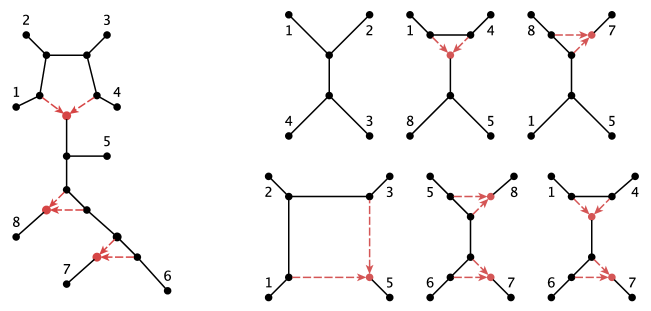
Figure 1: A phylogenetic network and 6 of the quarnets it displays. The quarnets from left to right: top row (quartet, single reticulation (1), single reticulation (2)), bottom row (square, double reticulation (1), double reticulation (2))

We denote a set of quarnets by $\mathcal{Q}$. If quarnets in a set can appear as restrictions of the same parent network, we say $\mathcal{Q}$ is a compatible set of quarnets. We refer to the set of all quarnets displayed by a parent network $N$ as the complete quarnet set which we denote $\mathcal{Q}(N)$. The goal of the main two algorithms in this article is to reverse this process by constructing a network from a complete quarnet set.

3 Sequential Algorithm

In this section, we present the first of our two network building algorithms. The sequential algorithm constructs an $n$-leaf network from its complete quarnet set by starting with one quarnet and then adding one leaf at a time in a location determined by a voting procedure. The resultant network is independent of both the choice of initial quarnet and order of leaves added.

3.1 Leaf Attachments Determine Networks

A leaf may be attached to a network in three different ways by inserting a new leaf edge or inserting a new semi-directed cycle of length 3 or greater. Collectively, the three moves comprise the set of single leaf attachments. We will later prove that the single leaf attachments can be used to construct any network via the sequential building algorithm.

Let $N$ be a network on $i$ leaves. To construct a network $N^{\prime}$ with $i+1$ leaves, we must add a new leaf, $x$. We define three functions $M_{k}(N,x,E)=N^{\prime}$ where $k=1,2,3$ to add a single leaf to $N$ at location $E$. The second attachment $M_{2}$ also has an extra parameter $r$ to specify the orientation of the reticulation event. The three attachments are pictured in Figure 2.

Definition 1

Single Leaf Attachment Functions Given a network $N$ we define the three single leaf attachments.

1. Insert a leaf edge ($M_{1}$) - Given an edge $e=\{u,v\}$ on $N$, we define a network $N^{\prime}=M_{1}(N,x,e)$ as follows. Introduce new vertices $w$ and $x$. Replace the edge $e$ with the pair of edges $\{u,w\}$ and $\{w,v\}$, and connect the new leaf by introducing the edge $\{w,x\}$.

   If $e$ was not a reticulation edge, then all new edges are undirected. If $e$ was a reticulation edge then without loss of generality, let $v$ be the reticulation vertex. Then $\{w,v\}$ is a reticulation edge and $\{u,w\}$ and $\{w,x\}$ are undirected.

2. Create an underlying 3-cycle ($M_{2}$) - Given an edge $e=\{s,t\}$ not on a cycle of $N$, we define a network $N^{\prime}=M_{2}(N,x,e,r)$ as follows. Insert vertices $u,v,w$ and $x$. Replace the edge $e$ with the set of edges $\{s,u\},\{u,v\}$ and $\{v,t\}$. To form a 3-cycle add the edges $\{v,w\},\{u,w\}$ and $\{w,x\}$.

   Given the 3-cycle, one of $u,v,w$ is a reticulation vertex as determined by the parameter $r\in\{u,v,w\}$. The two edges in the set $\{\{u,w\},\{w,v\},\{u,v\}\}$ incident with the reticulation vertex are reticulation edges directed towards the reticulation vertex. The third edge incident to the reticulation vertex is the out edge but is left undirected. All other new edges are undirected.

3. Create a larger underlying cycle ($M_{3}$) - Given two edges $e_{1}=\{p,q\}$ and $e_{2}=\{s,t\}$ on $N$ such that the path between $e_{1}$ and $e_{2}$ is not incident with any cycle of $N$, we define a network $N^{\prime}=M_{3}(N,x,e_{1},e_{2})$ as follows. Introduce two interior vertices $u$ and $v$ as well as reticulation vertex $w$ and new leaf $x$. Replace the edge $e_{1}$ with the pair of edges $\{p,u\}$ and $\{u,q\}$ . Replace the edge $e_{2}$ with the pair of edges $\{s,v\}$, and $\{v,t\}$. Add directed edges $\{u,w\}$ and $\{v,w\}$ directed towards $w$, as well as the out edge $\{w,x\}$.

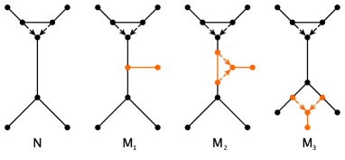
Figure 2: Each of the three single leaf attachments $M_{1},M_{2}$ and $M_{3}$ applied to a network $N$.

The edge restrictions in $M_{2}$ and $M_{3}$ ensure that the new cycles constructed by a leaf attachment are disjoint from the cycles on the original network. Therefore the resultant network of a leaf attachment on a level-1 network is itself level-1.

A network $N$ can be realized by a sequence of leaf attachments if the network can be built by describing a base quarnet and a series of leaf attachments that results in $N$. To show that a sequence of leaf attachments can realize every network, we must first show that a network must have either an out leaf or a tree cherry.

Lemma 1

Every network with at least four leaves contains an out leaf or a tree cherry.

Proof

Let $N$ be a network with a least four leaves. Root $N$ at a valid root location $\rho$ and direct all edges away from the root. This means internal vertices are either in-degree 1 and out-degree 2, or in the case of a reticulation vertex, in-degree 2 and out-degree 1.

Choose a leaf $l$ which maximizes the length of the path between the leaf and $\rho$. Since there are at least four leaves, $l$ must be adjacent to a non-root vertex $v$. If $v$ is a reticulation vertex, then $l$ is an out leaf since the orientation induced by a valid root must be consistent with the existing oriented edges.

Otherwise $v$ must have out-degree $2$. Since $l$ had the longest path to $\rho$, $v$ must be incident to a second leaf and is, therefore, a tree cherry. ∎

The previous lemma builds toward the central theorem for the leaf attachments. We use the fact that all networks have either a tree cherry or an out leaf to prove that all networks can be constructed via the leaf attachments.

Theorem 3.1

Every network with at least four leaves can be realized as a sequence of leaf attachments.

Proof

We proceed by induction on the number of leaves. Consider a network with 4 leaves. As $N$ itself is a quarnet, no attachments are required to build the 4-leaf network. Assume that all $n$-leaf networks can be built from a quarnet and a sequence of the single leaf attachments. We show that all $(n+1)$-leaf networks can be built from an $n$-leaf network and one single leaf attachment $M_{1},M_{2},$ or $M_{3}$.

Consider an arbitrary $(n+1)$-leaf network $N^{\prime}$. By Lemma 1, $N^{\prime}$ has a tree cherry or an out leaf.

If there is at least one tree cherry, arbitrarily choose a leaf on one tree cherry, call it $x$, and designate $x$ as the $(n+1)$th leaf of $N^{\prime}$. From $N^{\prime}$, we can determine an $n$-leaf network $N$, by removing $x$ and its incident edge. Then, suppress the degree 2 vertex that was adjacent to $x$ in $N^{\prime}$. Let $e$ be the edge in $N$ created by suppressing the degree 2 vertex. Apply the inductive hypothesis to assume that $N$ can be realized as a sequence of leaf attachments. Then use the first single leaf attachment to construct $N^{\prime}=M_{1}(N,x,e)$.

If there is no tree cherry, then $N^{\prime}$ has an out leaf by Lemma 1. Call the out leaf $x$ let it be the $(n+1)$th leaf of $N^{\prime}$. We construct an $n$-leaf network $N$ from $N^{\prime}$ by removing $x$, the edge incident to $x$, the reticulation vertex $r$ adjacent to $x$, and its reticulation edges. By removing the reticulation edges, there are now two degree 2 vertices. We consider two cases depending on whether $r$ is on a 3-cycle on $N^{\prime}$ or if $r$ is on a larger cycle.

If $r$ is on a 3-cycle, then the two degree 2 vertices are adjacent to each other. Thus, they are incident to the same underlying edge $e\in E(N)$. Suppress the degree 2 vertices. We now have our network $N$ and apply the inductive hypothesis to $N$. Construct $N^{\prime}$ from $N$ by $M_{2}(N,x,e,r)=N^{\prime}$.

Otherwise, if $r$ is on a larger cycle, then the two degree 2 vertices are not adjacent and therefore incident with 2 distinct underlying edges $e_{1},e_{2}\in E(N)$. Suppress the degree 2 vertices. The resulting network is $N$, and we apply the inductive hypothesis to $N$. Construct $N^{\prime}$ from $N$ by $M_{3}(N,x,e_{1},e_{2})=N^{\prime}$. Thus, $N^{\prime}$ can always be built from $N$ by one of $M_{1},M_{2},M_{3}$. Therefore, our statement is true by induction. ∎

3.2 Sequential Algorithm

By Theorem 3.1, we can determine a base quarnet and a sequence of attachments to build a network $N$ if we have access to $N$. However, the sequence can also be extracted directly from the complete set of quarnets.

The process involves choosing one of the quarnets as a base and sequentially adding the remaining leaves to the existing network. For a network with $|E|$ edges, there are $4|E|+{|E|\choose 2}$ potential attachments including the differing orientations of $M_{2}$. We introduce a voting procedure to determine which of these attachments is consistent with the input set of quarnets.

Definition 2

Sequential Voting Procedure For a network $N$, let $x$ be the leaf to be attached by a single leaf attachment. Let $\mathcal{Q}(x)$ be the set of quartets whose support includes $x$. An attachment $M$ is allowed on $N$ by $q$, if the network constructed by that attachment displays $q$. The optimal attachment is the attachment that is allowed by all $q\in\mathcal{Q}(x)$.

The process determines the correct attachment because the quarnet set is compatible. We can iterate this process to construct a network from quarnets.

Input: A complete set of quarnets $\mathcal{Q}(N)$ on $n$ leaves

Output: A unique $n$-leaf network $N$

Assign an arbitrary ordering to the set of leaves $X$ on $\mathcal{Q}(N)$ such that $X=\{x_{1},\dots,x_{n}\}$

Let $N_{4}$ be the quarnet with support $\{x_{1},x_{2},x_{3},x_{4}\}$

for $i\leftarrow 4$ to $n-1$ do

       Apply the voting procedure to the set $\mathcal{Q}(x_{i+1})$ to determine the optimal leaf attachment

      Perform that attachment to $N_{i}$ to determine $N_{i+1}$

Algorithm 2 Sequential Algorithm

Thus, any network can be built from its complete quarnet set by the sequential algorithm. We now work through an example of using the sequential algorithm to construct an 8-leaf network . The complete set of quarnets for an 8-leaf network consists of 70 quarnets. As such, not all quarnets are presented explicitly, and we reference only the quarnets shown in Figure 3.

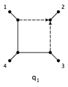
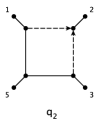
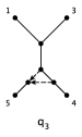
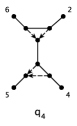
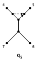
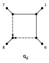
Figure 3: A subset of the complete quarnet set.

Let the leaf ordering be numerical (i.e. $1,2,\dots 8$). Our base quarnet has
$supp(q_{1})=\{1,2,3,4\}$. Let this quarnet be the first intermediate network $N_{4}$. Now, we look to place leaf $5$. Find the subset of quarnets that contain leaf 5 and three of leaves $1,2,3$, and $4$. We now let the appropriate quarnets vote to determine the attachment and its location.

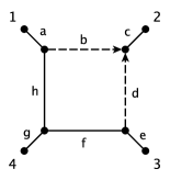
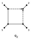
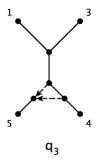
Figure 4: Intermediate network $N_{4}$ and two voting quarnets

We first consider the quarnet with $supp(q_{2})=\{1,2,3,5\}$ which is the second input quarnet in Figure 3. Recognize that for any quarnet, the attachment $M_{3}$ is between a pair of edges, but the path between any pair necessarily contains an edge on a cycle. Thus, performing $M_{3}$ would increase the level, so we only need to consider attachments $M_{1}$ and $M_{2}$.

Consider first all possible locations for attachment $M_{1}$. If we consider the order of the vertices, as defined by their adjacency to other leaves on the cycle, we cannot determine the relative order between leaves 4 and 5 from the base quarnet and the voting quarnet. Thus in Figure 4, $M_{1}$ may place leaf 5 on edges $f,g$ or $h$. As for $M_{2}$, the only potential $M_{2}$ attachment is on edge $g$ although all orientations are possible. As we have multiple allowed attachments from $q_{2}$, we must now consider another quarnet $q_{3}$.

Now consider the allowed attachments by the third quarnet in Figure 3 with $supp(q_{3})=\{1,3,4,5\}$. Notice that $q_{3}$ does not allow $M_{1}$ on any edge of $N_{4}$ because any restriction after performing the $M_{1}$ attachment would be a square quarnet. In fact, this quarnet only allows one attachment, $M_{2}(N_{4},5,g,w)$. By definition, all quarnets must allow the optimal attachment. Therefore, because this quarnet only allows one attachment, $M_{2}(N_{4},5,g,w)$ must be the optimal attachment and we need not consider other quarnets to determine $N_{5}$.

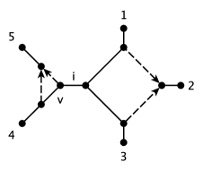
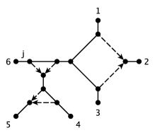
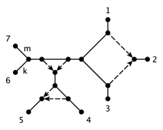
Figure 5: Intermediate networks $N_{5}$, $N_{6}$, $N_{7}$ determined by the quarnets in Figure 3

Perform $M_{2}(N_{4},5,g,w)$ to determine $N_{5}$. For the remainder of the example, we specifically choose to discuss quarnets in the complete quarnet set with the property that they only allow one move. The sequence of intermediate networks is shown in Figure 5.

To determine $N_{6}$, the fourth quarnet in Figure 3 with $supp(q_{4})=\{2,4,5,6\}$ allows only $M_{2}(N_{5},6,i,v)$ because leaf 6 cannot be on the same cycle as leaves 2,4, or 5. To determine $N_{7}$, the fifth quarnet in Figure 3 with $supp(q_{5})=\{4,5,6,7\}$ allows only $M_{1}(N_{6},7,j)$ because no new cycle needs to be added and if leaf $7$ is attached to any other leaf then the restriction would have to have 2 reticulation vertices. Finally, we determine $N_{8}$ which is our reconstructed network $N$. The final quarnet in Figure 3 with $supp(q_{6})=\{1,6,7,8\}$ allows only $M_{3}(N_{7},8,k,m)$ because leaves $6$ and $7$ are a cherry in $N_{7}$ but opposite leaves on the cycle on the quarnet. The resultant network $N$ is shown in Figure 6.

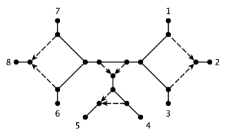
Figure 6: The resultant network $N$ determined by the quarnets in Figure 3

4 Cherry-Blob Algorithm

4.1 Cherry-Blob Algorithm Overview

Phylogenetic trees can be constructed using cherry-picking methods to peel off tree cherries and recursively build up trees cherrypicking2 . Networks can be constructed analogously by peeling off exterior structures. We propose the cherry-blob algorithm for reconstructing networks in this fashion from the complete set of quarnets.

The cherry-blob algorithm works by identifying exterior structures of networks and storing them. As shown in Figure 7, an exterior structure, $A_{S}$, partitions the leaves into $S$ and $X\setminus S$, where the leaves in $S$ are all adjacent to either a common vertex (if $A_{S}$ is a tree cherry) or a common semi-directed cycle (if $A_{S}$ is a reticulation cherry or an exterior blob).

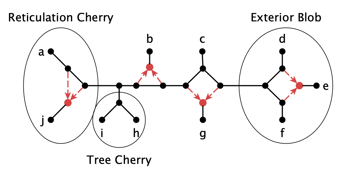
Figure 7: The three types of exterior structures found on networks.

The stem of an exterior structure $A_{S}$ is the non-trivial cut edge, $\{u,v\}$, that whose removal partitions the leaves. Call $v$ the stem tip if $v$ is adjacent to the leaves of a cherry, or $v$ is a vertex on the semi-directed cycle (if $A_{S}$ is a reticulation cherry or an exterior blob). The other vertex $u$ is the stem base. The subgraph $A_{S}$ contains the stem tip and every path between the stem tip and a leaf in $S$. The stem tip is the only degree 2 vertex on $A_{S}$. The stems of these exterior structures are the markers for cutting and gluing together networks.

A network $N$ can be modified by cutting or inserting exterior structures. The two operations are defined as $C$ for cutting an exterior structure and $I$ for inserting an exterior structure. The operations are used to show that a series of insertions can describe any network if the exterior structures are known.

Definition 3

Let $A_{S}$ be an exterior structure on a network $N$ with stem base $u$ and stem tip $v$. Then $C(N,A_{S})$ is the network constructed by removing $A_{S}$ from $N$, and then inserting a placeholder leaf $a_{S}$ along a new edge $\{u,a_{S}\}$. This is the cut procedure.

Definition 4

Let $A_{S}$ be an exterior structure with stem tip $v$. Let $l$ be a leaf on network $N$ and $u$ the vertex of $N$ adjacent to $l$. Then $I(N,l,A_{S})$ is constructed by removing $l$, adding $A_{S}$, and replacing the edge $\{u,l\}$ with the edge $\{u,v\}$. This is the insertion procedure.

The cut and insertion procedures are inverses of each other. Moreover, since any cycle in $A_{S}$ is disjoint from any other cycle in $N$, the cut or insertion of a level-1 structure is still level-1.

Definition 5

Let $A_{1},\dots,A_{k}$ be exterior structures with stem tips $v_{1},\dots,v_{k}$, and let $Z$ be a network with at least 4 leaves. Then $I(Z\mid A_{1},\dots,A_{k})$ is an insertion sequence defined by recursively inserting the exterior structures. We let $N_{0}=Z$, and $N_{i}=I(N_{i-1},v_{i},A_{i})$ for $1\leq i\leq k$. The resulting network $N_{k}$ is $I(Z\mid A_{1},\dots,A_{k})$.

Similarly, we define a cut sequence.

Definition 6

Let $N$ be a network with at least one exterior structure, and let $A_{1},\dots,A_{k}$ be an ordered list of subgraphs of exterior structures with stem tips $v_{1},\dots,v_{k}$. Then $C(N\mid A_{1},\dots,A_{k})$ is a cut sequence defined by recursively cutting the exterior structures. Let $Z_{0}=N$ $Z_{i}=C(Z_{i-1},v_{i})$ for $1\leq i\leq k$. Then the resulting network $Z_{k}$ is $C(N\mid A_{1},\dots,A_{k})$ which does not have any $A_{i}$ as a subgraph.

Now we outline how any network can be described as an insertion sequence. First, we observe that given a network $N$, we can determine a cut sequence to remove exterior structures until we arrive a base $Z$ that is either a quarnet or a sunlet (see Figure 8 for an example).

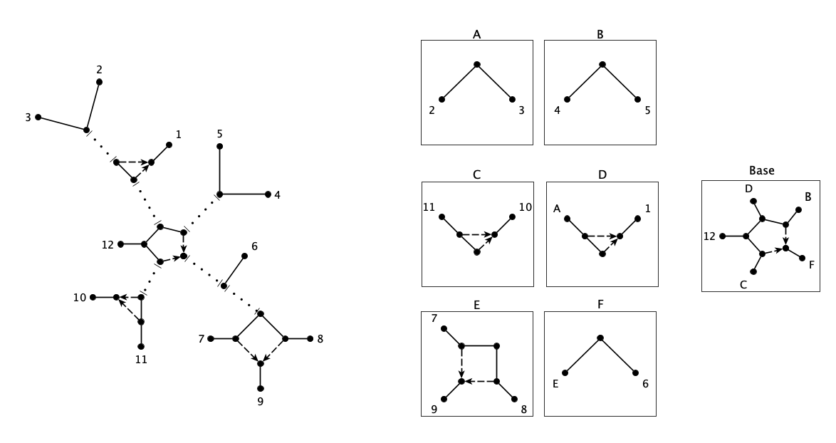
Figure 8: Left: A network with all non-trivial cut edges identified. Right: An ordered set of exterior structures and base that determine the network on the left.

Theorem 4.1

Every network $N$ with four or more leaves can be represented by an insertion sequence with a quarnet or a sunlet base.

Proof

We induct on the number of non-trivial cut edges in a network. If there are no non-trivial cut edges in $N$ then by definition, the network is a sunlet. Now assume that every network with at least four leaves and $k$ non-trivial cut edges can be written by an insertion sequence with a quarnet or sunlet base. Given a network $N$ with $k+1$ non-trivial cut edges, we first ask if it is a quarnet. If it is a quarnet, we finish. If not, then there must be an exterior structure $A_{S}$ such that $X\setminus S$ contains at least three leaves. Define a network $N^{\prime}$ by replacing $A_{S}$ with a leaf $l$. Since $N^{\prime}$ has at least four leaves and $k$ non-trivial cut edges then $N^{\prime}$ can be represented by an insertion sequence with a quarnet or sunlet base. The claim follows by observing that $N=I(N^{\prime},l,A_{S})$. ∎

Although up to this point we have assumed we know $N$, in practice, this is not the case. Then the goal of the following sections is to explain how any exterior structure can be identified from quarnets. We show that we can construct a unique network $N$ by an insertion sequence constructed from $\mathcal{Q}(N)$.

4.2 Reconstructing Exterior Structures of Networks

Recall an $n$-sunlet has $n$ leaves and one semi-directed cycle of length $n$. The symmetry of a sunlet makes it easy to analyze all of the quarnet restrictions (see figure 9).

Theorem 4.2

An network $N$ is an $n$-sunlet if and only if $\mathcal{Q}(N)$ consists of ${n-1}\choose{3}$ squares and ${n-1}\choose{4}$ quartet trees.

Proof

Let $N$ be an $n$-sunlet. Then it has $n$ leaves and an $n$-length cycle with exactly one reticulation event. By Lemma 1 one of the leaves must be an out leaf. The restriction to any quarnet containing this out leaf is a square, and the restriction to any quarnet not containing an out leaf is a quartet tree (see Figure 9). So there are ${n-1}\choose 3$ quarnets with the out leaf, which are squares, and ${n-1}\choose 4$ quarnets without the out leaf, which are quartet trees.

Now assume that $\mathcal{Q}(N)$ consists of $n-1\choose 3$ squares and ${n-1}\choose 4$ quartet trees for some network $N$. Since there is at least one reticulation vertex in the quarnets, there must be at least one reticulation vertex in $N$, so $N$ is not a tree. Assume for contradiction that $N$ is not a sunlet. Then $N$ must either have a tree cherry or another cycle.

If $N$ has a tree cherry, then it follows from the restriction process that there is at least one single reticulation quarnet which contains both the reticulation vertex and the tree cherry in the complete quarnet set. If $N$ has another cycle, then by the restriction process there is at least one double reticulation quarnet which contains two reticulation vertices.

In either case, $\mathcal{Q}(N)$ has quarnets that are not squares or quartets which is a contradiction. Therefore, $N$ must be a sunlet. ∎

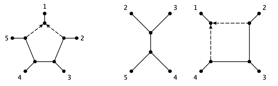
Figure 9: Left: a sunlet network. Right: examples of the two topologies of quarnet restrictions.

Thus we can identify when a network is a sunlet based on counting the number of squares and trees in $\mathcal{Q}(N)$. Moreover, we can identify both the location of the reticulation and the ordering of the leaves along the sunlet based on $\mathcal{Q}(N)$. The process for finding this ordering is similar to the sequential algorithm in that we start with a single square quarnet and add one leaf at a time based on information from other quarnets. The process is described in Algorithm 3.

Input: Let $\mathcal{Q}_{sq(N)}\subset\mathcal{Q}(N)$ be the set of square quarnets in the complete quarnet set of a sunlet network $N$.

Output: The placement of the reticulation vertex and the ordering of the leaves of $N$.

Pick $q\in\mathcal{Q}_{sq(N)}$. Set $B_{4}=q$.

for $i\leftarrow 4$ to $n-1$ do

      

      Pick a quarnet $q_{i+1}$ such that $|supp(q_{i+1})\cap supp(B_{i})|=3$, and two of the common leaves, $x_{a}$ and $x_{b}$, are incident to the same edge $e=\{v,w\}$ in $B_{i}$ and not incident to the same edge in $q_{i+1}$.

      Add a new vertex $u$.

      Replace the edge $e$ with the pair of edges $\{v,u\}$ and $\{u,w\}$.

      Let $x_{i+1}$ be the element in $supp(q_{i+1})\setminus supp(B_{i})$.

      Add an edge $\{u,x_{i+1}\}$.

      Call this new network $B_{i+1}$.

Algorithm 3 Sunlet Construction

The sunlet construction algorithm is even more powerful. If a set of leaves $X^{\prime}$ form the leaves of an exterior blob of a network $N$, and $y$ is any other leaf, then the restriction $N_{|X^{\prime}\cup\{y\}}$ is a sunlet, and thus the exterior structure can be reconstructed from the subset of $\mathcal{Q}(N)$ whose support is contained in ${X^{\prime}\cup\{y\}}$ using the sunlet construction method.

However, to do so would require knowing in advance which subsets of leaves form the leaves of the exterior structures or checking all $2^{n}$ possible subsets of leaves. We, therefore, need a strategy for determining which of the subsets of the leaves are contained in an exterior structure. Once this has been identified, one can reconstruct the exterior structure using the sunlet reconstruction algorithm. Our goal here is to identify a collection of subsets of leaves which could be the support of exterior blobs. To do so, we introduce an incompatibility graph.

Definition 7

For a network $N$ with leaf set $X$, let $H(\mathcal{Q}(N))$ be the incompatibility graph with vertex set $V=X$. Define an edge between leaves $a$ and $b$ if there exists single or double reticulation quarnet $q\in\mathcal{Q}(N)$ such that $\{a,b\}\subset supp(q)$ and there is a non-trivial cut edge on the path between $a$ and $b$ on $q$ (see Figure 10).

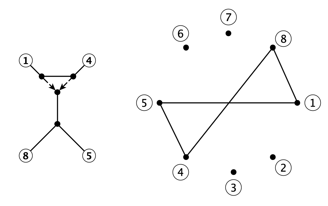
Figure 10: A single reticulation quarnet contributes 4 edges to the incompatibility graph

Consider a minimal vertex coloring of $H(\mathcal{Q}(N))$. Notice that the coloring is unique because each vertex in a color class is adjacent to all vertices in every other color class. The leaves of an exterior blob must be contained in a unique color class as no edge could connect them, and every non-element of the exterior blob would be connected to each leaf in the blob. Thus the leaves in each color class of a minimal vertex coloring of $H(\mathcal{Q}(N))$ are candidates to be exterior blobs. To determine if the leaves in a color class $X^{\prime}$ form an exterior blob, pick one leaf $y$ that is not in the color class and check if the quarnets which have support in $X^{\prime}\cup\{y\}$ are associated to a sunlet network. Thus the graph $H(\mathcal{Q}(N))$ allows us to check a maximum of $n$ sets for exterior structures rather than the potential $2^{n}$ subsets.

Unlike exterior blobs, which require a bit of effort to identify, cherries can be identified simply by counting quarnets.

Theorem 4.3

A network $N$ has a cherry containing leaves $a$ and $b$ if and only if $\mathcal{Q}(N)$ contains ${n-2}\choose 2$ quarnets with a cherry containing $a$ and $b$.

Proof

If $N$ has a cherry containing leaves $a$ and $b$, then it follows from the restriction process that $a$ and $b$ must be contained on a cherry on any quarnet on which they appear together. That will be ${n-2}\choose 2$ quarnets.

Now assume that ${n-2}\choose 2$ quarnets have a cherry containing leaves $a$ and $b$. Then $a$ and $b$ are contained on a cherry on every quarnet on which they appear together. It follows that no path on the network between $a$ and $b$ contains a non-trivial cut edge. Furthermore, the path between $a$ and $b$ and any two other leaves contains a non-trivial cut edge because there is a non-trivial cut edge between $a$ and $b$ and any two other leaves on some quarnet. Then there exists a cut edge on the network that partitions the leaf set into $\{a,b\}$ and all other leaves, so $a$ and $b$ are contained on a cherry. ∎

Consequently, all exterior structures of $N$ can be identified from the complete quarnet set.

4.3 Cherry-Blob Algorithm

Now that we can identify exterior structures from quarnets, we must find an way to order the structures such that an insertion sequence can be performed which attaches all of the structures to form $N$. We recursively identify an exterior structure $A_{S}$ from $\mathcal{Q}(N)$ then use Algorithm 4 to refine $\mathcal{Q}(N)$ to reflect the quarnet set for the network that results from cutting $A_{S}$ from $N$.

Input: A complete set of quarnets $\mathcal{Q}(N)$

Output: A complete set of quarnets on $\mathcal{Q}(C(N,A_{S}))$

1. Set $\mathcal{Q}(C(N,A_{S}))=\{\}$

2. for $q\in\mathcal{Q}(N)$ do

       if  $supp(q)\cap S=\{\}$ then

             $\mathcal{Q}(C(N,A_{S}))=\mathcal{Q}(C(N,A_{S}))\cup q$

      else if $supp(q)\cap S=\{s\}$ then

            Define $q^{\prime}$ as the quarnet $q$ with $s$ replaced with $a_{S}$

            $\mathcal{Q}(C(N,A_{S}))=\mathcal{Q}(C(N,A_{S}))\cup q^{\prime}$

      

Algorithm 4 Quartet Refinement Procedure

The quartet refinement procedure allows us to iterate the process of cutting exterior structures one at a time until either we are down to a single quarnet or the quarnet set for a sunlet. A terminal quarnet set is a complete quarnet set which contains either a single quarnet or only squares and quartets. We keep track of the exterior structures that have been cut along the way so that, so we can construct an insertion sequence beginning with the base to build the parent network. Algorithm 5 formalizes this iterative process.

Input: A complete set of quarnets $\mathcal{Q}(N)$

Output: The network $N$

$\mathcal{Q}=\mathcal{Q}(N)$

$i=0$

while $\mathcal{Q}$ is not a terminal quarnet set do

       while There exists a cherry in $\mathcal{Q}$ (See Theorem 4.3) do

             $i=i+1$

             Identify the stem tip $a_{S_{i}}$ of the cherry $A_{S_{i}}$

            $\mathcal{Q}=\mathcal{Q}(C(N,A_{S_{i}}))$

      Compute $H(\mathcal{Q})$

      Use color classes of $H(\mathcal{Q})$ to determine if there is an exterior blob

      if There exists an exterior blob then

             $i=i+1$

            Identify the stem tip $a_{S_{i}}$ of a single exterior blob $A_{S_{i}}$

            $\mathcal{Q}=\mathcal{Q}(C(N,A_{S_{i}}))$ using Algorithm 4

      

if $\mathcal{Q}$ is single quarnet then

       Call the quarnet $Z$

else

      Use Algorithm 3 to find the sunlet defined by $\mathcal{Q}$ and call it $Z$

Perform the insertion sequence $I(Z\mid A_{S_{k}},\dots,A_{S_{1}})$ using base $Z$, exterior structures $\{A_{S_{1}},...,A_{S_{k}}\}$ and leaf set $\{a_{S_{k}},\dots,a_{S_{1}}\}$ such that each $A_{S_{i}}$ replaces leaf $a_{S_{i}}$

Algorithm 5 Cherry-Blob Algorithm

5 Conclusion

The sequential and cherry-blob methods construct unrooted, semi-directed networks from a complete set of semi-directed quarnets. These two methods demonstrate that their restrictions to semi-directed quarnets uniquely determine semi-directed level-1 networks. These also extend the results of gambette2012quartets , which show that certain undirected level-1 networks can be constructed from their displayed quartets. This result is particularly interesting in light of the work of Gross and Long, which demonstrates that the semi-directed topologies can be recovered from sequence data under the Jukes-Cantor model gross . Together these articles provide a theoretical basis for constructing networks directly from sequence data.

Given the estimation error in identifying quarnets from sequence data, practical applications of these theoretical findings will likely require extensions of our algorithms to enable useful computations in the presence of quarnet error. The computational constraints involved in computing all $n\choose 4$ quarnets suggest the need for adaptations of these algorithms which require only a subset of the complete quarnet set. Those interested in such advances might first examine similar improvements to quartet based tree reconstruction such as those found in Maxcut ; EQS ; astral ; moan2015combinatorics ; qtetpuzzling among others.

Both types of extensions should be possible with the sequential method. Errant quartets could be handled by a modification of the voting procedure which selects the attachment that is best supported by the available quarnets, instead of the attachment supported by all quarnets. Also, we observed that often a single quarnet is sufficient for determining the allowed attachment. This fact suggests a study of decisive or definitive quarnets in an analogous manner to those undertaken for quartets could lead to significant algorithm efficiencies. Chapter 4 of steel2016phylogeny provides an excellent overview of these ideas.

Extending the cherry-blob method would require developing a statistical measure for detecting the presence of an exterior structure. There are well-established methods which detect tree cherries cherrypicking . The incompatibility graph can be modified such that edges are weighted by their occurrence, allowing for a reasonable prediction for the leaves of an exterior blob. While likely challenging as a theoretical problem, it is possible that the heuristic approaches would be useful in practice.

Finally, we note this work highlights the importance of studying networks which contain 3-cycles. These networks have been excluded from efforts to reconstruct networks from quartet trees (e.g. allman2019nanuq ; Huber2018 ; snaq ), but here play a fundamental role in constructing more extensive networks. In particular, even if one does not wish to allow 3-cycle networks in the final product, one might still have to allow 3-cycle networks in the restrictions.

Conflict of interest

The authors declare that they have no conflict of interest.

References

- (1) Elizabeth Allman, Hector Banos, and John Rhodes. Nanuq: A method for inferring species networks from gene trees under the coalescent model. arXiv preprint arXiv:1905.07050, 2019.
- (2) Jin-Hwan Cho, Dosang Joe, and Young Rock Kim. Quartet consistency count method for reconstructing phylogenetic trees. Communications of the Korean Mathematical Society, 25(1):149–160, 2010.
- (3) Tal Dagan. Phylogenomic networks. Trends in microbiology, 19(10):483–491, 2011.
- (4) R. Davidson, M. Lawhorn, J. Rusinko, and N. Weber. Efficient quartet representations of trees and applications to supertree and summary methods. IEEE/ACM Transactions on Computational Biology and Bioinformatics, 15(3):1010–1015, May 2018.
- (5) Philippe Gambette, Vincent Berry, and Christophe Paul. Quartets and unrooted phylogenetic networks. Journal of bioinformatics and computational biology, 10(04):1250004, 2012.
- (6) E. Gross and C. Long. Distinguishing phylogenetic networks. SIAM Journal on Applied Algebra and Geometry, 2(1):72–93, 2018.
- (7) Katharina T. Huber, Vincent Moulton, Charles Semple, and Taoyang Wu. Quarnet inference rules for level-1 networks. Bulletin of Mathematical Biology, 80(8):2137–2153, Aug 2018.
- (8) Jesper Jansson and Wing-Kin Sung. Inferring a level-1 phylogenetic network from a dense set of rooted triplets. Theoretical Computer Science, 363(1):60–68, 2006.
- (9) S. Mirarab, R. Reaz, Md. S. Bayzid, T. Zimmermann, M. S. Swenson, and T. Warnow. ASTRAL: genome-scale coalescent-based species tree estimation. Bioinformatics, 30(17):i541–i548, 08 2014.
- (10) Emili Moan and Joseph Rusinko. Combinatorics of linked systems of quartet trees. Involve, a Journal of Mathematics, 9(1):171–180, 2015.
- (11) Charles Semple Peter J. Humphries, Simone Linz. Cherry picking: A characterization of the temporal hybridization number for a set of phylogenies. Bull Math Biol, 75(10):1879–1890, 2013.
- (12) Sagi Snir and Satish Rao. Quartet maxcut: A fast algorithm for amalgamating quartet trees. Molecular Phylogenetics and Evolution, 62:1–8, 2011.
- (13) Ané C Solís-Lemus C, Bastide P. Phylonetworks: A package for phylogenetic networks. Molecular Biology and Evolution, 34(12):3292–3298, 2017.
- (14) Mike Steel. Phylogeny: discrete and random processes in evolution. SIAM, 2016.
- (15) K Strimmer and A von Haeseler. Quartet Puzzling: A Quartet Maximum-Likelihood Method for Reconstructing Tree Topologies. Molecular Biology and Evolution, 13(7):964–964, 09 1996.
- (16) Katharina T. Huber, Leo van Iersel, Remie Janssen, Mark Jones, Vincent Moulton, Yukihiro Murakami, and Charles Semple. Rooting for phylogenetic networks. arXiv e-prints, pages 1–25, 2019.